R E S E A R C H A R T I C L E
Open Access
Convergence study of the
h
-adaptive PUM
and the
hp
-adaptive FEM applied to
eigenvalue problems in quantum
mechanics
Denis Davydov
1*, Tymofiy Gerasimov
2, Jean-Paul Pelteret
1and Paul Steinmann
1*Correspondence:
[email protected] 1Chair of Applied Mechanics,
University of Erlangen-Nuremberg, Egerlandstr. 5, 91058 Erlangen, Germany
Full list of author information is available at the end of the article
Abstract
In this paper theh-adaptive partition-of-unity method and theh- andhp-adaptive finite element method are applied to eigenvalue problems arising in quantum mechanics, namely, the Schrödinger equation with Coulomb and harmonic potentials, and the all-electron Kohn–Sham density functional theory. The partition-of-unity method is equipped with an a posteriori error estimator, thus enabling implementation of error-controlledadaptivemesh refinement strategies. To that end, local interpolation error estimates are derived for the partition-of-unity method enriched with a class of exponential functions. The efficiency of theh-adaptive partition-of-unity method is compared to theh- andhp-adaptive finite element method. The latter is implemented by adopting the analyticity estimate from Legendre coefficients. An extension of this approach to multiple solution vectors is proposed. Numerical results confirm the theoretically predicted convergence rates and remarkable accuracy of theh-adaptive partition-of-unity approach. Implementational details of the partition-of-unity method related to enforcing continuity with hanging nodes are discussed.
Keywords: Adaptive finite element method, Partition-of-unity method, Error estimators, Schrödinger equation, Local interpolation error estimates, Density functional theory
Introduction
Recently there has been an increase of interest in applying finite element (FE) methods to
partial differential equations (PDEs) in quantum mechanics [1–14]. In order to improve
the accuracy of the solution, the basis set can be adaptively expanded through either
refinement of the mesh (h-adaptivity) or the basis functions can be augmented by the
introduction of higher polynomial degree basis functions (p-adaptivity). Since the solution
is not smooth and contains cusp singularities, the application of the h-adaptive FEM
may require very fine meshes and could be computationally inefficient. There are several approaches to circumvent this problem.
From the physical point of view, for ab initio calculation of molecules often core electrons (as opposed to valence electrons) behave in a similar way to single atom solutions. Thus
©The Author(s) 2017. This article is distributed under the terms of the Creative Commons Attribution 4.0 International License (http://creativecommons.org/licenses/by/4.0/), which permits unrestricted use, distribution, and reproduction in any medium, provided you give appropriate credit to the original author(s) and the source, provide a link to the Creative Commons license, and indicate if changes were made.
one possesses an a priori knowledge of a part of the solution vectors to the eigenvalue problem. One of the approaches used to introduce this into a FE formulation is the
partition-of-unity method (PUM) [15–17], which is a generalization of the classical FE
method. In PUM the enrichment functions are introduced into a basis as products with standard FE shape functions, thereby enlarging the standard FE space. As the standard FE functions satisfy the partition-of-unity property (that is, they sum to one in the whole domain), the resulting basis can reproduce enrichment functions exactly. For an overview
on PUM applied to continuum mechanics we refer the reader to [18–20].
An alternative approach to the above is to combineh- andp-adaptivity resulting in what
is termed ashp-adaptive FEM. For an overview ofhp-adaptive refinement strategies we
refer the reader to [21]. The general idea is that when the exact solution is smooth on the
given element,p-adaptive refinement is more efficient and leads to a faster convergence
with respect to the number of degrees of freedom; whereas if the solution is non-smooth
(singular),h-adaptive refinement is performed. Thus in addition to a reliable error estimate
and the choice of the marking strategy of elements for refinement,hp-adaptive methods
need to decide which type of refinement to perform on a given element. In this work we
use methods based on smoothness estimation [22–27]. As those methods are normally
employed for problems with a single solution vector, we propose an extension to multiple solution vectors as is required for the here considered eigenvalue problems.
Herein, our main focus is application ofh-adaptive PUM to PDEs in quantum mechanics,
namely to the Schrödinger equation and the all-electron density functional theory (DFT)
[28,29]. Application of the PUM to the above problems holds a significant promise to
improve on accuracy of a standard (non-enriched) FE approximation. The corresponding
numerical evidence can be found in [9], where convergence studies for PUM solutions
obtained onuniformlyrefined meshes are performed.
The novelty of our paper is that the PUM will be equipped with an a posteriori error
estimator, thus enabling implementation of error-controlledadaptivemesh refinement
strategies. Derivation and implementation of the PUM in computational solid mechanics is nowadays very well-acknowledged and established area of research, yet the authors are
not aware of any other work which applies theh-adaptive PUM to DFT.
We will also compare the PUM tohp-adaptive FEM in terms of the efficiency with
respect to the number of degrees of freedom. Although there are publications on the topic
ofhp-adaptive FEM applied to DFT [1], they lack any numerical studies and are limited
to a pre-defined refinement strategy of hexahedra that admit nuclei only at its vertices. In
order to apply thehp-adaptive FEM to DFT, in this paper we propose an extension of the
smoothness estimate approach using Legendre coefficients [22–25] to multiple solutions
vectors.
The outline of this paper is as follows: In the section on “Theory”, we introduce the eigenvalue problem studied here. The PUM and error estimators are also discussed. We
also explain the strategy employed to decide betweenh- andp-adaptive refinement for
thehp-adaptive FEM. Results of numerical studies of the chosen systems are presented
in section titled “Results and discussion”, followed by some conclusions. In Appendix A we rigorously derive the local interpolation error estimates for enrichment with a class of exponential functions; Appendix B describes the approach applied to solve single atom DFT in radial coordinates within application of the PUM; Appendix C discusses
Theory
In quantum mechanics we seek theNlowest eigenpairs (λα,ψα) of the Schrödinger
equa-tion [31]
−1
2∇
2+V(x)
ψα(x)=λαψα(x) on,
ψα(x)=0 on∂, (1)
ψα(x)ψβ(x)dx=δαβ.
Hereαis the index of the eigenpair,is a Lipschitz domain1inR3andδαβis the Kronecker
delta . In Kohn–Sham all-electron density functional theory [28,29], the potentialV(x)
depends on eigenvectors thus rendering the problem nonlinear. For a molecular system
consisting ofNeelectrons and M nuclei of charges{ZI}located at the (fixed) positions{RI},
the ground state electron densityρ(x) :=Nα=1fαψα(x)2can be obtained by finding the
N lowest eigenpairs of Eq. (1). Herefα is the partial occupancy number2of theα-orbital
such thatNα=1fα =Ne,V = Vion+VHartree+Vxcis composed of the ionic potential
Vion= −MI=1|x−ZIRI|, the Hartree potentialVHartree=
ρ(x)/|x−x|dx, and the (given)
exchange-correlation potentialVxc(ρ). As a result, the potentialVdepends on the density
ρ which is given in terms of eigenvectors{ψα}, making the problem nonlinear. From
practical perspectiveVHartreeelectrostatic potential is obtained by solving the associated
Laplace equation; together with (1) they are solved sequentially untill convergence in
density fieldsρis attained. For further details on the FE solution of DFT, we refer to our
previous work [2] and literature cited therein.
The weak form of Eq. (1) reads3
1
2∇v· ∇ψα+vVψα
dx=λα
vψαdx ∀v ∈H
1 0(),
ψαψβdx=δαβ.
(2)
We then introduce a FE triangulationPhofand the associated FE space of continuous
piecewise elements of a fixed polynomial degree :ψα ∈Vh⊂H01(). The FE solution to
the problem is then defined by
1
2∇v
h· ∇ψh
α+vhVψαh
dx=λhα
v
hψh
αdx ∀vh∈Vh,
ψh
αψβhdx=δαβ.
(3)
1Note that in the non-periodic case the Schrödinger equation is actually set inR3. Therefore the domainin Eq. (1)
is assumed to be sufficiently large such that zero Dirichlet boundary conditions make sense and there is no additional error due to considering a bounded domain. For all example systems that are considered below, the eigenfunctions are known to have asymptotic exponential decay which allows one to choose moderately sized domains.
2For spin unpolarized systems with an even number of electronsf
α≡2andN=Ne/2.
Partition-of-unity method
The classical FEM with piecewise linear ansatz spaces requires very fine meshes for ade-quate accuracy when the solution is not smooth or is highly oscillatory; this increases the computational cost of solving the problem. The PUM proposed by Melenk and Babuska
in [15,16] can address this issue. The main feature of the PUM is the inclusion of an a
priori knowledge about the solution properties into the FE space. The PUM enriches the
vector space spanned by standard FE basis functionsNi(x) (e.g. polynomials) by products
of these functions with functionsfj(x) that contain a-priori knowledge about the solution
ψh
α(x)=
i∈I
Ni(x)
⎡ ⎣ψi
α+
j∈S
fj(x)ψαij
⎤
⎦. (4)
Hereψαi are standard degrees-of-freedom (DoFs) andψαijare additional DoFs associated
with the shape functionsNi(x) and the enrichment functionsfj(x);I is a set of all nodes
andSis the set of enrichment functions. Since (possibly global) enrichment functionsfj(x)
are multiplied withNi(x) which has local support, the product also has local support and
therefore matrices arising from the weak form remain sparse. Also, since the standard
shape functions satisfy the partition of unity propertyiNi(x)≡1, the resulting vector
space can reproduce enrichment functionsfj(x) exactly.
Note that (4) is a more general approach than enriching the basis with fj alone (i.e.
without multiplying byNi, as is employed in [32]). Granted the partition of unity property
ofNi, this case can be obtained from (4) by requiring all DoFs associated with a given
enrichment functionfjto have the same value.
Error estimator
A posteriori error estimation analysis for FE approximations of (second-order) eigen-value problems has been a topic of intensive study within the last several decades, both from theoretical and implementational standpoints. We refer the interested reader to
[13,14,33–39], where two “conventional” types of error estimators, namely residual- and
averaging-based error estimators, are presented.
In general, a discretization error in approximated eigenfunctions,ψ−ψh, measured in a
suitable norm (e.g.L2-norm and energy norm, induced by the bilinear form of a problem),
as well as in approximated eigenvalues,|λ−λh|, can be estimated from above. That is,
ψ−ψh≤C1η, (5)
and
|λ−λh| ≤C2η2, (6)
whereC1, C2are the so-called stability constants that are independent of the mesh size
andηis theexplicitly computable4error upper-bound, see e.g. [34,38] for details. These
equations are typically termed(global) error estimators. The boundηreads as
η:=
⎡
⎣
K∈Ph
η2 K
⎤ ⎦ 1 2
,
where summation is performed over all elements inPhandηKis the(local) error indicator,
a quantity showing a discretization error of{ψh,λh}element-wise, that is, on every fixed
K. With multiple solutions available (in this case, eigenpairs{ψαh,λhα}),ηK will be a sum
of discretization errors of the corresponding eigenpairs on a given elementK, that is
ηK :=
α
η2 K,α
1 2
.
For a standard (non-enriched)Q1-based finite element solution of (1), a local indicator
ηK,αofresidualtype reads as follows (see [13,14,34,35,38,39] for details):
η2 K,α :=h2K
K −
1
2∇
2+V(x)
ψh
α−λhαψαh
2
dx
+hK
e⊂∂K
e
−1
2∇ψ
h
α ·n
2
e
da, (7)
where [[−12∇ψαh·n]]e:=
−1
2∇ψαh|K +12∇ψαh|K
·nerepresents the jump of the gradient
across interfaceebetween two adjacent elementsKandK,neis the outward unit normal
vector toeandhK :=diam(K).
One of the key findings of our work is the proof that indicator (7) also holds (with no
modification due to the enrichment usage) in the PUM with the exponential enrichment
function f(x) = exp (−μ|x|k). In Appendix A, we derive and prove the related local
interpolation error estimates required for the derivation of the error indicator (7).
hp-adaptive solution
There have been numerous works devoted to hp-adaptive refinement [22–25,40–42]
including a comparison of different methods [21]. The main difficulty thata posteriori
hp-adaptive methods aim to address is the following: once an error is estimated and a
certain subset of elements is marked for refinement, one has to choose between h- or
p-refinement for each element. In this work we adopt anhp-refinement method based
on the estimate of the analyticity of the solution5on the reference element via expansion
into Legendre bases [22–25]. In particular, the FE solution is analytic on elementKif, and
only if, there exists constantsCK andσK such that
aKijk≤CKexp(−σK[i+j+k]), (8)
where aijk are Legendre coefficients; see [25] for further details. We chose to estimate
the decay coefficient σK by performing a least squares fit of Legendre coefficients in
each direction lnaKd,i∼lnCKd−σKdifor 1≤i≤pK, and then use the minimum decay
coefficient as the final valueσK =mindσKd. WhenσKvalue is below a chosen parameterσ0,
the solution is considered to be smooth atKand thusp-refinement is performed, otherwise
h-refinement is executed. For initially linear FEsp-refinement is always performed. We
note that methods based on the decay rate of the expansion coefficients were found in [21]
to be the best choice as a general strategy for thehp-adaptive solution of elliptic problems.
To the best of our knowledge there is, however, very little (numerical) study of those
methods applied to DFT. The only paper we are aware of [1] lacks any numerical results.
We also note that, in the majority of cases,hp-adaptive FEM is applied to problems inR1
andR2. Thus we also aim to evaluate how well the smoothness estimators proposed in the
literature work for eigenvalue problems inR3that are relevant to quantum mechanics.
In order to extend thishp-refinement strategy to the eigenvalue problem, that is when
there are multiple vectors represented using the same FE basis, we propose the following approach. For each element we find an eigenvector which contributes the most to the total element’s error. The smoothness of this vector is the basis on which we decide
to perform h-refinement orp-refinement. The rationale behind this approach is that
we aim at minimizing the error the most during a single refinement step while being
conservative and avoiding performing both h- and p-refinement on the same element.
We also investigated allowing bothh- andp-adaptive refinement of a single cell based on
smoothness estimation of all eigenvectors, but ultimately found that this procedure leads to qualitatively similar results for the problems studied herein.
Finally, for the error indicator we adopt the following expression [43]
η2 K,α:=
h2K p2K
K −
1
2∇
2+V(x)
ψh
α−λhαψαh
2
dx
+
e⊂∂K
he
2pe
e
−1
2∇ψ
h
α·n
2
e
da, (9)
where he is the face’s diameter, pK is the element’s polynomial degree and pe is the
maximum polynomial degree over two elementsKandKadjacent to the facee.
The derivation of the error estimators for hp-FEM usually requires the polynomial
degree of neighbouring elements to be comparable, namely that there existsγandsuch
thatγpK ≤ pK ≤ pK for all elements K, K that have a non-empty intersection. In
order to reflect this assumption in our numerical scheme, we propose that an additional step which limits the differences in polynomial degrees among elements be performed.
More precisely, afterhp-adaptive refinement is executed, then for each elementK, we
find the maximum polynomial degree among its neighbouring elements pmaxneigh and if
pmaxneigh>pK +2 then we setpK ←pK +1.
Results and discussion
If not explicitly stated otherwise, the results below are obtained for the following
con-figuration: (i) the initial polynomial degree for non-enriched DoFs is one forhp-adaptive
FEM; (ii) linear shape functions are used in PUM to introduce enrichments, higher order elements were not employed as the interpolation error estimates are derived only for
lin-ear elements and thus limit the applicability of the error indicator stated in Eq. (7) ; (iii) a
Gaussian quadrature rule with 203points is used for enriched elements in the eigenvalue
problem; (iv) the Dörfler marking strategy withθ = 0.6 is used to mark elements for
refinement; (v) Gauss–Legendre–Lobatto supports points are used for the hp-adaptive
highest polynomial degree is limited to 8 for computational efficiency reasons; (vii) the radius in which enriched FEs are employed is heuristically chosen for each numerical
example; (viii) following [25] we chooseσ0=1.0 as a parameter in the smoothness
esti-mator.6Implementation details of the partition-of-unity method indeal.II[30] finite
element library are given in Appendix C.
Schrödinger equation
In this section we consider the Schrödinger equation Eq. (1) with two different (spherical)
potentialsV(x)=V(|x|).7The first case is the Coulomb potentialV(x)= −1/|x|, which
corresponds to a Hydrogen atom. The eigenvalues of this problem are degenerate. InR3,
on each energy levelnthere aren2eigenvaluesλn=λ1/n2, whereλ1= −1/2 [31]. The
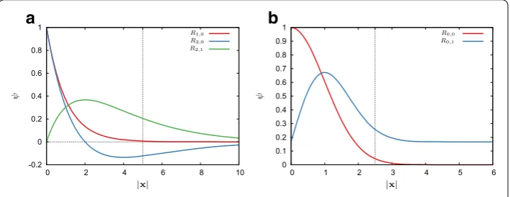
eigenfunction corresponding to the lowest eigenvalue reads
ψ1(x)= √1
π exp (− |x|). (10)
The radial component of the eigenfunctions at the next energy level are R2,0 = [1−
|x|/2] exp(− |x|/2) andR2,1= |x|/2 exp(− |x|/2).
The second potential we will consider is a harmonic potentialV(x)= |x|2/2 that leads
to a harmonic oscillator problem. The eigenvalues for this problem are also degenerate; in
R3they are given byλn=n+1/2 fornth energy level. The lowest two have a degeneracy
of 1 and 3, respectively. The (unnormalized) eigenfunction corresponding to the lowest eigenvalue is
ψ1(x)=exp− |x|2/2. (11)
The radial component of the next eigenfunction isR0,1(x)= |x|exp
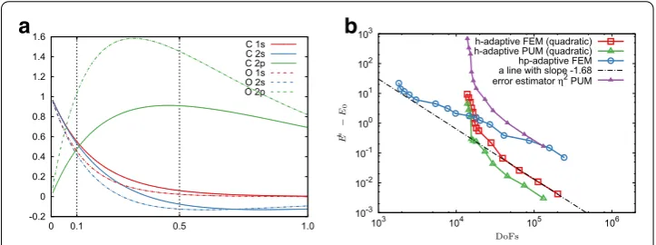
− |x|2/2. Figure1
shows radial components of eigenfunctions for the Coulomb and the harmonic potential. It is clear that in order to have a low interpolation error for a standard Lagrange FE basis, a very fine mesh will be required near the origin. For such non-smooth solutions we will see that by introducing enrichment functions the interpolation error of the resulting FE basis will be greatly reduced.
The initial mesh used to solve the Schrödinger equation is obtained from 3 global mesh
refinements of the single element in = [−20; 20]3 for the Coulomb potential and
=[−10; 10]3for the harmonic potential. For the PUM only 8 elements adjacent to the
singularity that is located at the origin are marked for enrichment.
First, we examine the convergence in case when a single eigenpair is required in the
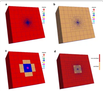
Schrödinger equation with two different potentials. Figure 2 compares the h-adaptive
FEM,hp-adaptive FEM andh-adaptive PUM, whereas Fig.3shows the cross-sections of
meshes for the last refinement step.
For both combinations of potentials and enrichment functions, theh-adaptive PUM is
superior toh-adaptive FEM. In particular, for the last refinement step the PUM solution is
about two orders more accurate than theh-adaptive FEM with the same number of DoFs
in the case of the Coulomb potential. For the harmonic potential this value is smaller. The
6Note that in [22] the Legendre coefficients were required to have even slower decay rate ofσ
0=0.69.
7For spherically symmetric potentials one can separate eigenfunctions into radialR
-0.2 0 0.2 0.4 0.6 0.8 1
0 2 4 6 8 10
|x|
ψ
R1,0
R2,0
R2,1
a
0 0.1 0.2 0.3 0.4 0.5 0.6 0.7 0.8 0.9 1
0 1 2 3 4 5 6
|x|
ψ
R0,0
R0,1
b
Fig. 1 Radial components of eigenfunctions for different potentialsV(x). The dotted vertical line indicates the smallest initial mesh size which will be used in our numerical calculations.aCoulomb.bHarmonic
10-5 10-4 10-3 10-2 10-1 100 101
103 104 105
h-adaptive FEM (linear) hp-adaptive FEM h-adaptive PUM h-adaptive FEM (quadratic) a line with slope -1.88 a line with slope -0.79
DoFs
λ
h−0
λ0
a
10-8 10-6 10-4 10-2 100 102
102 103 104 105
h-adaptive FEM (linear) hp-adaptive FEM h-adaptive PUM h-adaptive PUM (larger enrichment domain) a line with slope -0.75
DoFs
λ
h−0
λ0
b
Fig. 2 Error convergence rates for an eigenproblem with a single eigenpair.aCoulomb potential.
bHarmonic potential
asymptotic convergence rate of theh-adaptive PUM with the default enrichment radius
is very similar to that of theh-adaptive FEM for both problems (compare green and red
lines in Fig. 2), which supports our theoretical findings.
The advantage of the h-adaptive PUM also depends on the enrichment radius with
respect to the underlying exact solution. To examine this effect we employ an initial mesh obtained only by two global refinements of a single element and mark the 8 elements adjacent to the origin for enrichment. With this approach we effectively consider a larger
enrichment domain [−5; 5]3instead of [−2.5; 2.5]3. Importantly, the numerically
non-zero part of the underlying analytical solution will be almost fully contained in those 8
elements (see Fig.1b). From the numerical results we observe that for the most refined
stage theh-adaptive PUM displays an error which is about 6 orders of magnitude less than
the same method with the smaller enrichment domain (compare purple and green lines
in Fig.2b).
For the case of a single eigenpair, thehp-adaptive FEM performs remarkably well and,
unless a larger enrichment radius is used inh-PUM, it converges to the higher tolerance
with fewer number of DoFs (compare blue and green lines in Fig.2).
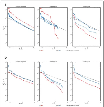
Now let us turn our attention to a more realistic scenario where one seeks multiple
eigenpairs whereby an a prioriknowledge is available only for the first eigenfunction.
degree
8 7 6 5 4 3 2 1 a
degree
8 7 6 5 4 3 2 1 b
degree
8 7 6 5 4 3 2 1
c d
Fig. 3 Cross-sections of the final adaptive meshes for the Coulomb potential when solving for a single eigenpair.ah-adaptive FEM (linear).bh-adaptive FEM (quadratic).chp-adaptive FEM.dh-adaptive PUM (linear)
the first 4 eigenvalues for the harmonic potential for the different methods. For both
problems thehadaptive PUM again has remarkable convergence properties, superior to
h-adaptive FEM. It is important to note that even though in the PUM the enrichment
function corresponds to the first eigenfunction only, other eigenpairs in the case of the
harmonic potential tend to converge faster than the standardh-adaptive FEM case, as can
be observed in Fig.4b. The same applies to the spherical orbital at the second energy level
of the Hydrogen atom; see Fig.4a where the corresponding eigenvalue in the PUM case
displays a faster convergence rate than the others on the same energy level.
For the Hydrogen atom, in the case of thehp-adaptive refinement one observes a
supe-rior convergence rate of the first eigenvalue, whereas eigenvalues from the next energy
level have errors that are comparable to theh-adaptive linear FEM. A possible issue could
be related to the smoothness estimation on elements with hanging nodes. In particular it
is observed [44] that the smoothness is overestimated when using similar methods, albeit
based on Fourier coefficients. This leads to unnecessarily high order polynomial degrees in these areas. Clearly, further investigation is required to resolve this problem.
Density functional theory
10-5
10-4
10-3
10-2
10-1
103 104 105
h-adaptive FEM (linear)
1 2-5 a line with slope -0.72
10-5
10-4
10-3
10-2
10-1
103 104 105
hp-adaptive FEM
10-5
10-4
10-3
10-2
10-1
103 104 105
h-adaptive PUM
DoFs DoFs
DoFs
λ
h α−
λα
a
10-6
10-5
10-4
10-3
10-2
10-1
100
101
103 104 105
h-adaptive FEM (linear)
1 2-4 a line with slope -0.84
10-6
10-5
10-4
10-3
10-2
10-1
100
101
103 104 105
hp-adaptive FEM
10-6
10-5
10-4
10-3
10-2
10-1
100
101
103 104 105
h-adaptive PUM
DoFs DoFs
DoFs
λ
h α−
λα
b
Fig. 4 Convergence of eigenvalues from the first two energy levels for the Schrödinger equation in the course of adaptive refinement. Red lines denote the lowest eigenvalue, whereas blue lines correspond to degenerate eigenvalues on the next energy level.aCoulomb potential (4 out of 5 eigenvalues are degenerate).bHarmonic potential (3 out of 4 eigenvalues are degenerate)
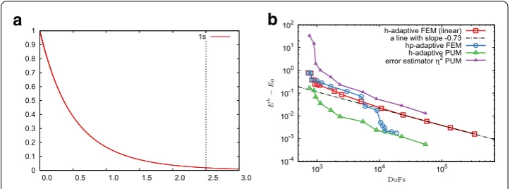
occupied state, i.e.Ne=2 andN =1. The ground state energy from the radial solution is
E0= −2.834289. Enrichment functions for PUM are obtained from numerical solution of
single atom Schrödinger equations, depicted in Fig.5a. The atom is placed at the origin in
the domain=[−10; 10]3with the homogeneous mesh of sizeh=2.5. Eight elements
adjacent to the atom are enriched.
Figure5b compares theh-adaptive FEM,hp-adaptive FEM andh-adaptive PUM. One
immediately recognizes that the PUM leads to a much faster convergence in terms of DoFs and gives about an order of magnitude advantage in terms of the absolute value of
the error. The linearh-adaptive FEM would require ten times more DoFs to achieve the
same accuracy. Thehp-adaptive FEM displays an exponential-like decay and approaches
the accuracy of PUM at higher number of DoFs.
In the second test problem we consider a CO molecule in the domain=[−10; 10]3
at the (equilibrium) distance 2.1. In order to estimate the ground state energy, we fit the
0 0.1 0.2 0.3 0.4 0.5 0.6 0.7 0.8 0.9 1
0.0 0.5 1.0 1.5 2.0 2.5 3.0 1s
a
10-4 10-3 10-2 10-1 100 101 102
103 104 105
h-adaptive FEM (linear) a line with slope -0.73 hp-adaptive FEM h-adaptive PUM error estimator η2 PUM
DoFs
E
h−
E0
b
Fig. 5 Finite element solution of He atom.aScaled radial solution. The dotted vertical line indicates the enrichment radius.bConvergence of the error in total energy of He atom for various FE methods
C+qln(DoFs) with constraintsC>0, E0<Eh, q<0. Using this approach we estimate
the limit of the ground state energy to beE0= −112.47107. This renders a bond energy8
of−0.5775, which compares favourably to the value−0.578 reported in [45]. This gives us
confidence to use the estimated ground state energy value in convergence studies, which
are presented in Fig.6.
The enrichment functions for PUM are obtained from the numerical solution of single atom Schrödinger equations; see Appendix B for details. The scaling of those functions are
not important for PUM, so Fig.6a depicts radial solutions normalized so that the value of
the 1sand 2sorbitals are unity at the origin. It is generally possible to use all eigenfunctions
from the radial solution as enrichments around each atom in the radius of a few atomic units. However, extra care must be taken not to render the resulting FE space to have
linearly dependent basis functions. Figure6a clearly indicates that given small enough
elements (on the order 0.1 a.u.), enriching with both 1sand 2s single atom radial core
electrons solutions would make the FE space degenerate. Our current implementation of PUM DFT only supports enrichment in non-overlapping domains. Therefore for the CO
molecule we have to start from a relatively fine mesh, which in the course ofh-adaptive
refinement may render the basis enriched with multiple functions linearly dependent. To avoid this, the PUM results for the CO molecule are obtained by enriching 8 elements
adjacent to each atom with its 1s orbital only. Scaling of the 1s function to unity at
the origin of the enrichment spherical function improves the condition number of the resulting matrices.
Figure6b compares the convergence characteristics using the h-adaptive FEM, hp
-adaptive FEM andh-adaptive PUM. The energy error convergence rate fromh-adaptive
FEM compares favourably to the expected rate of O(h2p), which can be approximated
byO(DoFs−2p/3). Remarkably, the chosen smoothness estimate used in thehp-adaptive
FEM and its extension to multiple vectors do not lead to an increase in efficiency in terms
of the number of DoFs as compared toh-adaptive quadratic FEM. Theh-adaptive PUM
displays the same convergence rate ash-adaptive FEM and is, as expected, more accurate.
This, however, comes at the expense of having a worse condition number for the resulting matrices and the necessity to use higher quadrature order to perform sufficiently accurate numerical integration. For this example and the chosen enrichment radius, the
-0.2 0 0.2 0.4 0.6 0.8 1 1.2 1.4 1.6
0 0.1 0.5 1.0
C 1s C 2s C 2p O 1s O 2s O 2p
a
10-3 10-2 10-1 100 101 102 103
103 104 105 106
h-adaptive FEM (quadratic) h-adaptive PUM (quadratic) hp-adaptive FEM a line with slope -1.68 error estimator η2 PUM
DoFs
E
h
−
E0
b
Fig. 6 Finite element solution of CO molecule.aScaled radial solution of single atoms. The dotted vertical line at 0.5 indicates the enrichment radius.bConvergence of the error in total energy of CO molecule for various FE methods
ence in energy error between the two approaches is less than one order of magnitude. By comparing these results to those presented earlier for H and He atoms, we hypothetize that a larger enrichment radius is required to make the PUM advantageous compared
to theh-adaptive FEM. Our current implementation of PUM DFT, however, only allows
enrichment in non-overlapping domains, which limited the enrichment radius for the CO example.
Conclusions
In this contribution we have applied and critically compared the h- and hp-adaptive
FEM, and theh-adaptive PUM to the relevant PDEs in quantum mechanics, namely the
Schrödinger equation and the Kohn–Sham all-electron density functional theory. The main findings are summarized below.
• The PUM renders several orders of magnitude more accurate eigenvalues than the standard FEM when solving the Schrödinger equation for the lowest eigenpair with Coulomb and harmonic potential. For the case when more eigenpairs are sought but only the lowest eigenvector is introduced as an enrichment, the PUM is still more accurate, especially for the lowest eigenvalue. Remarkably other eigenvalues also exhibit a faster convergence. The results from DFT calculations indicate that in order to keep this advantage, a reasonably large enrichment radius is needed.
• For problems where a single eigenpair is being sought, thehp-adaptive FEM with the
here considered smoothness and residual error estimators results in a more accurate
solution with fewer number of DoFs as compared to h-adaptive PUM and FEM.
However, for the case of multiple eigenpairs this approach did not lead to satisfactory
results. Overall we findh-adaptive PUM to be a more robust solution method to reach
the required accuracy even with relatively small enrichment domains.
• Local interpolation error estimates are derived for the PUM enriched with the class of exponential functions. In this case the results are the same as for the standard FEM
and thereby admit the usage of the error indicator (7).
• For the PUM DFT calculations the convergence rate of energy error and the residual error estimator are the same for all studied examples. Thus our numerical results
confirm that Eq. (7) can be considered as a reliable error indicator for problems in
• An element view to the implementation of PUM in FEM codes based on hexahedra is proposed (see Appendix C). As a result, continuity of the enriched field along the edges with hanging nodes is enforced by treating FE spaces produced by each func-tion in the local approximafunc-tion space separately. The resulting algebraic constraints are independent on the enrichment functions. This allows one to directly reuse algo-rithms written for enforcing continuity of vector-valued FE spaces constructed from a list of scalar-valued FEs.
Abbreviations
x: position vector;λα: eigenvalue;ψα(x): eigenvector;V(x): potential;: Lipschitz domain;Ph: triangulation of;Vh:
the finite element space of fixed polynomial degree;λh
α: eigenvalue obtained from the finite element solution of the
problem;ψh
α(x): eigenvector obtained from the finite element solution of the problem;ψαi: standard degrees-of-freedom;
Ni(x): finite element shape functions;fj(x): enrichment functions;ψαij: enriched degrees-of-freedom;η: explicitly computable error upper-bound;ηK: local error indicator on the elementK;ηK,α: local error indicator for eigenpairαon the elementK;aijk: Legendre coefficients;σK: the decay coefficient;he: the face diameter;pK: the element’s polynomial
degree;pe: the maximum polynomial degree over two elementsKandKadjacent to the facee.
Authors’ contributions
DD developed the concepts proposed and discussed in this manuscript, performed the numerical implementation and experiments and wrote the draft of this paper. TG derived local interpolation error estimates and improved the mathematical introduction of the problem. JPP contributed to the numerical implementation and paper revisions, and PS revised the paper. All authors read and approved the final manuscript.
Author details
1Chair of Applied Mechanics, University of Erlangen-Nuremberg, Egerlandstr. 5, 91058 Erlangen, Germany,2Institute of
Applied Mechanics, Technische Universitaet Braunschweig, Bienroder Weg 87, 38106 Braunschweig, Germany.
Acknowledgements Not applicable.
Competing interests
The authors declare that they have no competing interests.
Availability of data and materials Not applicable.
Consent for publication Not applicable.
Ethics approval and consent to participate Not applicable.
Funding
The support of this work by the ERC Advanced Grant 289049 MOCOPOLY (DD, JP, PS) and German Science Foundation (Deutsche Forschungs-Gemeinschaft, DFG), Grant DA 1664/2-1 (DD) is gratefully acknowledged. Second author (TG) is supported by the European Research Council (ERC) Starting Researcher Grant INTERFACES, Grant Agreement No. 279439.
Appendix A: Local interpolation error estimates
In this appendix, the local interpolation error estimates required for the derivation of the
error indicator (7) in the case of PUM are obtained for linear finite element approximations
enriched withf(x)=exp (−μ|x|p), where 0< μ∈Rand 1≤p∈N. These are
v−qhv
L2(K)≤cKhK|v|H1(ωK), (12)
v−qhv
L2(e)≤ceh 1 2
K|v|H1(ωK), (13)
where, as usual,v: → Ris a scalar-valued function, which is assumed to be at least
inH1(),qh is a quasi-interpolation operator (of the averaging type),K is an element
of the discretizationPhof,e ⊂ ∂K is an edge ofK. Also,hK measures the size ofK,
ωK is the patch of elements neighboringKincludingK itself. Finally,cK, ce ∈Rare the
We fix the notations to be used throughout the appendix and make assumptions that are conventional for this kind of analysis. For the sake of simplicity and without loss of generality, we elaborate here for the two-dimensional setting. The obtained results are valid in three dimensions as well.
First, we assume that the partitionPhof⊂R2consisting of open and convex
quadri-laterals K isshape-regular (ornon-degenerate), as well as locally quasi-uniformin the
sense of [46,47]. For everyKand its edgeewe definehK :=diam(K) andhe:= |e|is the
length ofe. For every nodeiinPhwe denote byωithe union of quadrilaterals connected
to nodei and sethωi := diam(ωi). Furthermore, for everyK,ωK represents the patch
containingKand the first row of its neighbors; it is then sethωK :=diam(ωK).
Also, in what follows, by the notationabwe imply the existence of a positive constant
C independent ofaandbsuch thata≤Cb. Thena∼ bmeans thata banda b
hold simultaneously. The symbol| · |will be used to denote either theH1-seminorm (as
e.g. in (12) and (13)) or thelengthof a linear segment inR2or theareaof a plane domain
in R2. With these notations at hand, one can show that|K|12 ∼ hK,|ωi|12 ∼ hω
i and
|ωK|12 ∼ hωK. Furthermore, the shape regularity of the meshPhensures thathe ∼ hK,
whereas its local quasi-uniformity implies thathK ∼hωi∼hωK.
Finally, we also recall useful inequalities, which are
• the Poincaré-type inequality (see e.g. [48]):
v− 1
|ω|
ωv dx
L2(ω)≤
hω
π |v|H1(ω), ∀v∈H1(ω), (14)
whereω⊂Rn(n=2,3) is a Lipschitz domain andhω:=diam(ω);
• the scaled trace inequality (e.g. in [49], Lemma 3.2):
vL2(e)h− 1 2
e vL2(K)+h 1 2
e |v|H1(K), ∀v∈H1(K). (15)
Quasi-interpolation operator
Herein, we construct an interpolation operator for obtaining the local error estimates (12)
and (13).
LetV :=H1() be an admissible space andVhbe its (enriched) finite element
coun-terpart
Vh:=
⎧ ⎨
⎩vh∈C() :vh(x) :=
i∈I
aiNi(x)+f(x)
i∈I
biNi(x)
+
i∈Istd.
ciNi(x), ai, bi, ci∈R
⎫ ⎬
⎭⊂V, (16)
where Iis the set of all enriched nodes ofPh andIstd. is the set of standard, i.e.
non-enriched nodes ofPh;I∩Istrd. = ∅. Recall also thatNi in our case is theQ1-shape
function associated with nodeiand supported onωi.
Explicit construction of the operator qh : V → Vh implies the explicit pattern of
approximation (16), the major challenge in deriving qh is imposition of the
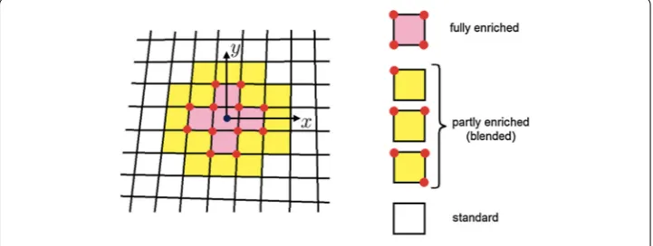
constant-preserving property onqh, which should be fulfilled on every elementK ∈Phregardless
the element type (see Fig.7).
The operatorqh:V →Vhwith the desired property reads as follows:
qhv(x) :=
i∈I
1 2|ωi|
ωi v(y)dy
Ni(x)+ f(x)
i∈I
1 2f(xi)|ωi|
ωi v(y)dy
Ni(x)
+
i∈Istrd.
1 |ωi|
ωi v(y)dy
Ni(x), (17)
with all notations as in (16) and wherexi, entering the second term, denotes the coordinate
of a nodei. Below, for the proposed quasi-interpolation operator of the averaging type
qhwe establish thatqhc|K = con a standard element (note this is a classical result for a
non-enriched FEM) and, more importantly, thatqhc|K =c+O(hpK) on a fully-enriched
and a blended element.
Estimates
Preliminaries
The three estimates that we start with are basic for the following local interpolation error
analysis. On everyK ∈Pkand its nodeiit holds that
Ni(x)L2(K)hK, Ni(x)L2(e)h 1 2
K, (18)
|ωi1|ω
i
v(y)dyh−K1vL2(ωK)+ |v|H1(ωK), (19)
and
f(x)
f(xi)=
1+O(hpK). (20)
Results (18) rigorously follow from the isoparametric concept and related properties, see
e.g. [50] for details. We note that they may be also derived in a less rigorous manner owing
to a boundedness of the basis functionNionKalong with|K|
1
2 ∼hKand|e|12 =h 1 2
e ∼h
1 2
K.
The inequality (19) is obtained as follows:
|ωi1|ω
i
v(y)dy≤ |ωi|−1
ωi
v(y)dy≤ |ωi|−12vL2(ω
i)
h−K1vL2(ωK)+ |v|H1(ωK).
Here we used the Cauchy–Schwarz inequality,|ωi|12 ∼hω
i∼hK and also the
extension-related resultvL2(ωi)≤ vL2(ωK).
Finally, to show (20) we explicitly use the properties off(x). For any fixedK,x∈Kand
xi∈Kbeing one of its nodes, we have the following upper bound estimate:
f(x)
f(xi)=
exp(μ|xi|p)
exp(μ|x|p) ≤
expμmaxx∈K|x|p
expμminx∈K|x|p ≤
expμminx∈K|x| +hK
p
expμminx∈K|x|p
=1+μp
min
x∈K |x|
p−1
hK +h.o.t.in
min
x∈K |x|
, hK
=1+O
min
x∈K|x|
p−1
hK
. (21)
Notice that due to boundedness of minx∈K|x|for a given fixedK, there always exists >0
such that minx∈K|x| =hK. Using this in (21), we obtain
min
x∈K |x|
p−1
hK =p−1hpK,
yielding, as a result, ff((xx)
i) ≤1+O(h
p K).
The lower bound estimate can be found similarly:
f(x)
f(xi)=
exp(μ|xi|p)
exp(μ|x|p) ≥
expμminx∈K|x|p
expμmaxx∈K|x|p ≥
expμminx∈K|x|p
expμminx∈K|x| +hK
p
=1−μp
min
x∈K |x|
p−1
hK +h.o.t.in
min
x∈K |x|
, hK
=1+O
min
x∈K|x|
p−1
hK
,
and, eventually, ff((xx)
i) ≥1+O(h
p
K). The result (20) then follows.
Stability of qhin L2-norm
The next step towards (12) and (13) implies obtaining the so-called stability result for the
constructedqh. Using (18)–(20) one straightforwardly shows that
qhv
L2(K)vL2(ωK)+hK|v|H1(ωK), (22)
and
qhv
L2(e)h
−1 2
K vL2(ωK)+h 1 2
K|v|H1(ωK). (23)
These estimates indeed hold for every K regardless of its type (standard, blended,
enriched). Note that for a standard non-enriched FEM and the resulting interpolation
operators, the estimates (22) and (23) are classical. We have obtained and proved them
Constant-preserving property of qh
The final ingredient required for obtaining (12) and (13) is the determination of how “well”
the constructedqhreproduces the constant on an elementK, depending on its type. This
constant-preserving property of the operator is of major importance particularly in the case of enriched FEM.
The required result on a standard (non-enriched) element K follows immediately.
Indeed, in this case
qhv(x)|K = 4
i=1
1 |ωi|
ωi v(y)dy
Ni(x),
and the partition of unity4i=1Ni(x)=1 onKyieldsqhc|K =c,c=const.
The situation on a fully-enriched and partly-enriched (blended) element is more delicate. In the case of a fully enriched element we have
qhv(x)|K = 4
i=1
1 2|ωi|
ωi v(y)dy
Ni(x)
+ f(x)
4
i=1
1 2f(xi)|ωi|
ωi v(y)dy
Ni(x),
that, owing to (20), results in
qhc|K =
1
2c+
1
2c
4
i=1
f(x)
f(xi)
Ni(x)=
1
2c+
1
2c
1+O(hpK)
4
i=1
Ni(x)=c+O(hpK).
Now, letK be a blended element, implying the representation:
qhv(x)|K =
i=1
1 2|ωi|
ωi v(y)dy
Ni(x)
+ f(x)
i=1
1 2f(xi)|ωi|
ωi v(y)dy
Ni(x)
+ 4
i=+1
1 |ωi|
ωi v(y)dy
Ni(x),
where∈ {1,2,3}is the number of enriched nodes ofK. Adding and subtracting the first
sum in the above expression, enables us to rewrite it as follows:
qhv(x)|K = −
i=1
1 2|ωi|
ωi v(y)dy
Ni(x)
+f(x)
i=1
1 2f(xi)|ωi|
ωi v(y)dy
Ni(x)
+ 4
i=1
1 |ωi|
ωi v(y)dy
Ni(x).
need to estimate, in this context, the remaining part constituting of the first and the second sums. We obtain,
qhc|K =
1
2c
i=1
f(x)
f(xi)−
1
Ni(x)+c≤
1
2c
i=1
ff((xxi))−1Ni(x)+c
≤ 1
2c
4
i=1
ff((xxi))−1Ni(x)+c=
1
2cO(h
p K)
4
i=1
Ni(x)+c=c+O(hpK),
where (20) was also used.
Proof of local error estimates (12), (13)
The derivation of the estimates forv−qhvL2(K)andv−qhvL2(e)is based on a
com-bined use of the above stability results forqh, the Poincaré and the scaled trace inequalities
(14) and (15), respectively, as well as the constant-preserving property results. First, due
to linearity ofqh, we have
v−qhv
L2(σ)=
v−c−qh(v−c)+c−qhc
L2(σ)
≤ v−cL2(σ)+qh(v−c)
L2(σ)+
c−qhc
L2(σ), (24)
wherec = const and where, for the sake of brevity, we setσ = {K, e}. We are now in a
position to dissect every term in (24) in either case ofσ.
Whenσ =Kin (24):
By the Poincaré inequality (14), it holds that
v−cL2(K)≤ v−cL2(ωK)hK|v|H1(ωK), (25)
where one can choosec= |ωK|−1ω
Kvdxand usehωK ∼hK.
By the stability estimate (22) and the Poincaré inequality, it holds similarly to the above
that
qh(v−c)
L2(K)v−cL2(ωK)+hK|v−c|H1(ωK)hK|v|H1(ωK). (26)
Furthermore, using the results of “Constant-preserving property ofqh” section we obtain
c−qhc
L2(K)≡0, ifK is standard, (27)
and
c−qhc
L2(K)=O(h
p+1
K ), ifKis fully enriched or blended. (28)
In the former case we also use that1L2(K)= |K|
1 2 ∼hK.
Using (25)–(28) in (24), the resulting local interpolation error of type (12) follows. Note
that in the case of fully enriched and blended elements the termO(hpK+1) that appears
in the corresponding upper bound can be neglected, being the higher order term with
respect to the leading onehK|v|H1(ωK).
By the scaled trace inequality (15), it holds
v−cL2(e)h− 1 2
e v−cL2(K)+h 1 2
e |v−c|H1(K)h 1 2
K|v|H1(ωK), (29)
where we also usehe∼hK along with result in (25).
By the stability estimate (23) and the Poincaré inequality (14), we obtain the result that
qh(v−c)
L2(e)h
−1 2
K v−cL2(ωK)+h 1 2
K|v−c|H1(ωK)h 1 2
K|v|H1(ωK). (30)
Finally, using the results of “Constant-preserving property ofqh” section we derive
c−qhc
L2(e)≡0, ifK is standard, (31)
and
c−qhc
L2(K)=O(h
p+1 2
K ), ifK is fully enriched or blended. (32)
In the former case we also use the fact that1L2(e)= |e|
1 2 =h
1 2
e ∼h
1 2
K.
Using (29)–(32) in (24), the resulting local interpolation error estimate of type (13)
follows as well. Again, in the case of fully enriched and blended elements the termO(h
3 2
K)
that appears in the corresponding upper bound can be neglected, being the higher order
term with respect to the leading oneh
1 2
K|v|H1(ωK).
Appendix B: Single atom radial solution
The radial solution of a single atom with chargeZ is obtained by solving the following
coupled problem 1 r2 d dr r2d
dr R
φ =4π ρ (33)
−1 2 1 r2 d dr r2d
dr +
[l+1]l
2r2 +V(ρ, r)
Rψnl =nlRψnl (34)
ρ=
n
l
2l+1
4π fnlR
ψ
nl 2
(35)
wherenandlare the main and azimuthal quantum numbers,fnlare occupation numbers,
V is the effective potential and Rψrl and Rφ are respectively radial components of the
eigenfunctions and electrostatic potential. The radial component of the eigenfunctions
are normalized by 0∞r2(Rψnl)2dr = 1. On the change of variables Unlψ := r Rψnl and
Uφ :=r Rφ, the system takes the form
d2
dr2Uφ =4πrρ (36)
−1
2
d2
dr2 +
[l+1]l
2r2 +V(ρ, r)
Unlψ =nlUnlψ (37)
ρ=
n
l
2l+1
4πr2 fnlU
ψ
nl 2
which together with the following Dirichlet boundary conditions
Unlψ(0)=0 (39)
Unlψ(∞)=0 (40)
Uφ(0)=0 (41)
Uφ(∞)=Z (42)
can be solved using the standard finite element method in a sufficiently large but finite
domain. The eigenfunctions are then given byψnlm = RψnlYlm, whereYlm are spherical
harmonics.
Appendic C: PUM implementational details
An enriched finite element class has been implemented for the general purpose
object-orientedC++finite element librarydeal.II[30]. The implementation is based on the
FESystemclass, which is used to build finite elements for vector valued problems from a list of base (scalar) elements. What differs from that class is that the developed FE implementation is scalar, but built from a collection of base elements and enrichment
functions9
u(x)=
i∈I
Ni(x)ui+
k∈S
fk(x)
⎡ ⎢
⎣
j∈Ikpum
Njk(x)ujk
⎤ ⎥
⎦, (43)
whereI is the set of all DoFs with standard shape functions (see Fig.8a),Ikpumis the set
of all DoFs corresponding to shape functions enriched withfk(x) (see Fig.8b) andSis the
set of enrichment functions.
As distribution of DoFs indeal.IIis element based, we always enrich all DoFs on
the element. To restore C0 continuity between enriched and non-enriched elements,
additional algebraic constraints are added to force DoFsujk associated withNjkfkon the
face between the enriched and non-enriched elements to be zero. This is equivalent to enriching only those shape functions whose support is contained within the enriched elements.
Theh-refinement indeal.IIis implemented using hanging nodes. In this case, extra
algebraic constraints have to be added to make the resulting field conforming. We build these constraints separately for the non-enriched FE shape functions and enriched shape
functions; that is, the following spaces are separately made conforming:{Ni(x)},{Nj0(x)},
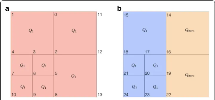
{Nj1(x)}, etc. To illustrate this idea consider two separate FE spaces shown in Fig.8.
We assume that functions in the first space are non-zero everywhere in the domain, whereas functions in the second space are non-zero only in the left part, marked by the blue shading. Therefore we do not have to introduce any DoFs in the right part,
the underlying elements are denoted by Qzero. The standard procedure implemented
in deal.II [27] will enforce continuity of the vector field by introducing algebraic
constraints for DoFs associated with hanging nodes10 (3,5,17,19), plus constraints for
9This is a generalization of (4) which allows to use different FE spaces for each enrichment function. In practice one
uses linear shape functions for enriched DoFs and possibly higher order shape functions for non-enriched DoFs.
10For linear FEs, the value at the hanging node is the average of the values at adjacent vertices, for exampleu
5 =
a
b
Fig. 8 Treatment of hanging nodes for theh-adaptive PUM.Q1denotes (bi)linear FE, whereasQzerodenotes
elements on which functions in the FE space associated with the enrichment functionfk(x) are zero and thus
no DoFs need to be introduced.aFirst FE space (standard).bSecond FE space (enrichment)
DoFs 14,16,22 to make functions in the second FE space zero at the interface between
Q1 andQzero. We can observe now that if we take the constrained scalar field from
the first FE space and add a scalar field from the second FE space multiplied by the
enrichment functions f(x) (continuous in space), the resulting scalar FE field will also
be continuous. Thus we arrive at a conformingh-adaptive PUM space where only some
elements are enriched. With reference to Fig.8, the resulting PUM field will have
enrich-ment associated with DoFs 23,24,20,21,17,18,15 whereas DoFs 22,19,16,14,17 will be
constrained.
In this procedure the algebraic constraints do not depend on the enrichment func-tions and are equivalent to those one would have for the vector-value bases build upon the same list of scalar FEs. Therefore, no extension of the existing functionality to build algebraic constraints was necessary. This allows us to reuse the code written for the
FESystem class, which can be used in deal.II to build a vector-valued FE from a collection of scalar-valued elements. Another remarkable benefit of this approach is
that existing code can be used to transfer the solution during h-adaptive refinement
from a coarse to a fine mesh. The reason is that prolongation matrices for enriched elements are equal to their vector-valued counterparts under the condition that all child elements are also enriched. Yet another advantage of implementing a dedicated
enriched finite element indeal.IIlibrary relates to the numerical integration of jump
terms in the Kelly error indicator (see “Error estimator” section). Here, care needs to be taken in computing contributions to cell errors from faces with hanging nodes. Had the authors pursued an implementation of PUM where values and gradients of addi-tional basis functions are evaluated manually via the product rule in the course of numerical integration, a completely separate function would have to be implemented to integrate the jump terms in error indicators, which is not a straight-forward task. We believe that the implementation outlined above is general enough to allow PUM to be
![Fig. 9 h -adaptive mesh refinement and shape functions associated with the central node on the domain[0, 1]2 for the standard and enriched element](https://thumb-us.123doks.com/thumbv2/123dok_us/9581266.1940923/22.595.119.479.85.197/adaptive-renement-functions-associated-central-standard-enriched-element.webp)
