R E S E A R C H A R T I C L E
Open Access
Recursive POD expansion for
reaction-diffusion equation
M. Azaïez
1*, F. Ben Belgacem
2and T. Chacón Rebollo
3,4*Correspondence:
1Bordeaux INP, I2M, (UMR CNRS
5295), 33607 Pessac, France Full list of author information is available at the end of the article
Abstract
This paper focuses on the low-dimensional representation of multivariate functions. We study a recursive POD representation, based upon the use of the power iterate
algorithm to recursively expand the modes retained in the previous step. We obtain general error estimates for the truncated expansion, and prove that the recursive POD representation provides a quasi-optimal approximation inL2norm. We also prove an exponential rate of convergence, when applied to the solution of the reaction-diffusion partial differential equation. Some relevant numerical experiments show that the recursive POD is computationally more accurate than the Proper Generalized
Decomposition for multivariate functions. We also recover the theoretical exponential convergence rate for the solution of the reaction-diffusion equation.
Keywords: Recursive POD, High Order SVD, Model Reduction, Multivariate functions, PGD
Background
Model Reduction methods are nowadays basic numerical tools in the treatment of large-scale parametric problems appearing in real-world problems. They are applied with suc-cess, for instance, in signal processing, analysis of random data, solution of parametric partial differential equations and control problems, among others. In signal processing, Karhunen-Loève’s expansion (KLE) provides a reliable procedure for a low dimensional representation of spatiotemporal signals (see [12,20]). Different research communities use different terminologies for the KLE. It is named the proper orthogonal decomposi-tion (POD) in mechanical computadecomposi-tion (see [3]), referred to as the principal components analysis (PCA) in statistics (see [17,18,24]) and data analysis or called singular value decomposition (SVD) in linear algebra (see [13]). These techniques allow large reduction of computational costs, thus making affordable the solution of many parametric problems of practical interest, otherwise out of reach. Let us mention some representative references [5,6,11,16,26,27], although this list, by far, is not exhaustive.
The extension of KLE to the tensor representation of multivariate functions is, how-ever, a challenging problem. Real problems are quite often multivariate. Let us mention, for instance the analysis of multivariate stochastic variables, simulation and control of thermal flows and multi-component mechanics, among many others. Some recent tech-niques have been introduced to build low-dimensional tensor decompositions of multi-variate functions and data. Among them, the High-Order Singular Value Decomposition
©2016 Azaïez et al. This article is distributed under the terms of the Creative Commons Attribution 4.0 International License (http:// creativecommons.org/licenses/by/4.0/), which permits unrestricted use, distribution, and reproduction in any medium, provided you give appropriate credit to the original author(s) and the source, provide a link to the Creative Commons license, and indicate if changes were made.
(HOSVD) provides low-dimensional approximation of tensor data, in a similar way as the Singular Value Decomposition allows to approximate bi-variate data (see [7,8,21]). Also, the Proper Generalized Decomposition (PGD) appears to be well suited in many cases to approximate multivariate functions by low-dimensional varieties (see [14,15]). However, in general there is not an optimal tensor of rank three or larger to approximate a given high-dimensional tensor (see [9]).
In this paper we study an alternative method to build low-dimensional tensor decom-positions of multivariate functions. This is a recursive POD (R-POD), based upon the successive application of the bivariate POD to each of the modes obtained in the previous step. In each step only one of the parameters is active, while the set of the remaining parameters is considered as a passive single parameter. We introduce a feasible version of the R-POD, in which the expansion is truncated whenever the singular values are smaller than a given threshold. This provides a fast algorithm, as only a small number of modes is computed, just those required to achieve a targeted error level.
As an application, we analyze the velocity of convergence of the R-POD applied to approximate the solution of the reaction-diffusion equation. We prove that the expansion converges with exponential rate. We use as main theoretical tool the Courant-Fischer-Weyl Theorem, that allows to reduce the error analysis of the POD expansion to that of the polynomial approximation of the function to be expanded. We also use the analytic dependence of the solution on the diffusivity and reaction rate coefficients, that yields the exponential convergence rate. This analysis is based upon the one introduced in [2]. Fur-ther, we use sub-sequent bounds for the singular values to construct a practical truncation error estimator, which is used to recursively compute the expansion by the Power Iterate (PI) method [1]. This avoids to compute the full singular value decomposition of the cor-relation matrix, just the modes needed to attempt a given error threshold are computed. The PI method provides a fast and reliable tool to build the POD expansion of bivariate functions, of which we take advantage to recursively build the R-POD expansion.
We present a battery of numerical tests, in which we apply the R-POD to the rep-resentation of three-variate functions, and in particular to the solution of the reaction-diffusion. We compare the R-POD to the PGD expansion. The PGD expansion can be interpreted as the PI method applied to the effective computation of the POD for bivari-ate functions (see [23]). We here consider its extension to multivariate functions. We obtain exponential convergence rates for both R-POD and PGD expansions, although the R-POD is in general more accurate than the PGD for the same number of modes. We also recover an exponential rate of convergence for the R-POD approximation of the solution of the reaction-diffusion equation, in quite good agreement with the theoretical expectations.
Notation—LetX⊂Rdbe a given Lipschitz domain andGa measure space. We denote byL2(G, X) the Bochner space of measurable and square integrable functions fromGon
X(cf. [10]).
The Karhunen-Loève decomposition on Hilbert spaces
The Karhunen-Loève decomposition, also known as Proper Orthogonal decomposition (POD in the sequel) provides a technique to obtain low-dimensional approximations of parametric functions. To describe it, let us consider a Hilbert spaceH endowed with a scalar product (·,·)H, and a parameter measure spaceG. Let us consider a function f ∈L2(G, H), and introduce the POD operator
A:H→H, Av=
G
f(γ) (f(γ), v)Hdγ forv∈H.
POD operator is linear and bounded. Moreover, it is self-adjoint and non-negative. Indeed, it holdsA=B∗B, whereB:H→L2(G) and its adjoint operatorB∗:L2(G)→H
are given by
(Bv)(γ)=(f(γ), v)H forv∈H,
B∗ϕ=(ϕ, f)L2(G)=
G
f(γ)ϕ(γ)dγ forϕ∈L2(G). (1)
Furthermore, the operatorAis compact. This arises because the operatorBis compact by the Kolmogorov compactness criterion inL2(G) (cf. Muller [22], Chapter 2).
Consequently, there exists a complete orthonormal basis ofHformed by eigenvectors (vm)m≥0 of A, associated to non-negative eigenvalues (λm)m≥0, that we assume to be
ordered in decreasing value. Each non-zero eigenvalue has a finite multiplicity, and 0 is the only possible accumulation point of the spectrum. IfHis infinite-dimensional, then limm→∞λm=0.
Moreover, consider the correlation operatorC=BB∗:L2(G)→L2(G),
Cϕ(γ)=
G
(f(γ), f(μ))Hϕ(μ)dμ forϕ∈L2(G).
Then the sequence (ϕm)m≥0, with
ϕm(γ)=
1
σm
(Bvm)(γ)=
1
σm
(f(γ), vm)H,σm=
λm(it also holdsvm=
1
σm B∗ϕm)
(2)
is an orthogonal basis ofL2(G). This yields the abstract Karhunen-Loève decomposition,
Corollary 0.1 It holds
f(γ)=
m≥0
σmϕm(γ)vm, a. e. in G,
where the series is convergent in L2(G, H).
The main interest of the POD is the following best-approximation property (cf. [22], Chapter 2):
Lemma 0.2 Let Vl=Span(ϕ1,. . .,ϕl)⊂H . Let Wlbe any sub-space of H of dimension l. Then
G
dH(f(γ), Vl)2dγ ≤
G
where
dH(v, Wl)= inf w∈Wl
v−wH for v∈H
denotes the distance from the elementϕ∈H to the sub-space Wl.
Let us next consider the case of bivariate functions. Assume thatX ⊂RdandY ⊂Rs
are two bounded domains,dandsare integers≥1. LetTbe a given function inL2(X×Y), that we want to approximate in a low-dimensional variety. Let us consider the integral operator with kernelT expressed as
v→B v, (B v)(y)=
X
T(x, y)v(x)dx. (3)
The operatorBmapsL2(X) intoL2(Y), is bounded and has an adjoint operatorB∗defined fromL2(Y) intoL2(X) as
ϕ→B∗ϕ, (B∗ϕ)(x)=
Y
T(x, y)ϕ(y)dy. (4)
We are thus in a particular case of the previous abstract setting, withG=Y,H =L2(X) andf(γ)(x)=T(x,γ).
Recursive POD representation
The POD expansion may be recursively adapted to the representation of multi-parametric functions. Let us consider the case of trivariate functions to avoid unnecessary complexi-ties. Consider a bounded domainZ⊂Rqfor some integer numberq≥1, and a trivariate functionT ∈L2(X×Y×Z). We identifyT with a function ofL2(Y ×Z, L2(X)) as both spaces are isometric. From Corollary0.1we deduce that there exist two orthonormal sets (vm)m≥0and (ϕm)m≥0which are respectively complete inL2(X) and inL2(Y ×Z) such
thatT admits the representation
T(x, y, z)=
m≥0
σmϕm(y, z)vm(x), (5)
where the sum is convergent inL2(Y×Z, L2(X)). Moreover the singular valuesσm(that
we assume to be ordered in decreasing value) are non-negative and converge to zero. We next apply the POD expansion to each modeϕm(y, z). There exists two orthonormal
sets (u(km))k≥1and (wk(m))k≥1which are respectively complete inL2(Y) andL2(Z), such that
ϕmadmits the representation ϕm(y, z)=
k≥0 σ(m)
k u
(m) k (y)w
(m)
k (z), (6)
where the expansion is convergent inL2(Z, L2(Y)), which is isometric toL2(Y×Z). Also, the singular values (σk(m))k≥0are non-negative and decrease to zero. We then haves
Lemma 0.3 The function T ∈L2(X×Y ×Z)admits the expansions
T =
m≥0
k≥0
σmσk(m)vm⊗uk(m)⊗wk(m)=
m≥0
σmvm⊗ ⎛
⎝
k≥0 σ(m)
k u
(m)
k ⊗w
(m) k
⎞ ⎠,
(7)
Proof It is enough to prove that any of both series is absolutely convergent. Consider the partial absolute sum for the first one
SN =
0≤m≤N
0≤k≤N
σmσk(m)vm⊗u(km)⊗wk(m)2L2(X×Y×Z).
As the eigenfunctions are orthonormal (in their corresponding spaces),
SN =
0≤m≤N
0≤k≤N
|σm|2|σk(m)|2≤
0≤m≤N
|σm|2≤ T2L2(X×Y×Z),
where the first inequality holds becauseϕmL2(Y×Z)=1, and then
k≥0 |σ(m)
k |2=1.
Feasible recursive POD representation
To build up a feasible recursive POD (R-POD) representation, consider a partial sum of the POD representation (7),
TPM =
0≤m≤M
σmvm⊗ ⎛
⎝
0≤k≤Km σ(m)
k u
(m)
k ⊗w
(m) k
⎞
⎠, (8)
for some given integersK1≥1,. . ., KM ≥1. The notationPMis a short for the multi-index
(M, K1,. . ., KM). We have
T−TPM 2
L2(X×Y×Z) =
m≥M+1 |σm|2
⎛
⎝
k≥0 |σ(m)
k |
2
⎞
⎠+
0≤m≤M
|σm|2
⎛
⎝
k≥Km+1 |σ(m)
k |
2
⎞ ⎠
≤
m≥M+1 |σm|2+
0≤m≤M
|σm|2
⎛
⎝
k≥Km+1 |σ(m)
k |
2
⎞
⎠ (9)
This estimate suggests a practical strategy for the IP method to construct the expansion (8) within a targeted error:
Algorithm FR-POD (Feasible recursive POD representation) Assume that some estimates of the remainders are computable:
m≥M+1
|σm|2≤ |αM|2,
k≥Km+1 |σ(m)
k |
2≤ |β(m)
K |2. (10)
Set a toleranceε >0. Let
A=1/√2, B=1/(√2TL2(X×Y×Z)). (11)
• Step 1: Compute the modesϕmandvmand singular valuesσmform =1,. . ., Mε,
untilαMε ≤Aε.
• Step 2: For eachm=1,. . ., Mε, compute the modesu(mk)andwk(m)and the singular
valuesσm(k)fork=1,. . ., Km, untilβK(mm)≤Bε.
For smooth functions the singular values decrease very fast, so that good estimators of the remainders areαM = σM+1,βK(m)=σKm+1. For less smooth functions, some more
summands of the series defining the remainders could be need. In “Analysis of solutions of the reaction-diffusion” section we shall obtain estimatorsαMandβK(m)whenTis the
Lemma 0.4 Let Tεthe representation of T provided by Algorithm FR-POD within an error levelε. It holds
T−TεL2(X×Y×Z)≤ε. (12)
Proof From estimate (9) and (10),
T−TPM2L2(X×Y×Z) ≤ |αMε|2+
0≤m≤M
|σm|2|βK(mm)|
2≤(A2+ T2
L2(X×Y×Z)B2)ε2< ε2, where we have used that
0≤m≤M
|σm|2≤ T2L2(X×Y×Z).
In practice we recursively compute the expansion by the PI method [1]. This avoids to compute the full singular value decomposition of the correlation matrix, we just compute the modes needed to reach a given error threshold.
Quasi-optimality of recursive POD representation
The POD representation in general provides the most accurate representation inL2norm, for a given number of truncation modes. This is due to the best-approximation property stated in Lemma0.2. Let us consider a trivariate approximation ofT withMmodes, of the form
ˆ
TM(x, y, z)=
0≤m≤M
ˆ
Xm(x) ˆYm(y) ˆZm(z), for (x, y, z)∈X×Y×Z. (13)
Lemma 0.5 Let T ∈L2(X×Y ×Z). It holds
T−TML2(X×Y×Z)≤ T −TˆML2(X×Y×Z), (14)
where
TM(x, y, z)=
0≤m≤M
σmϕm(y, z)vm(x), (15)
andTˆMis any trivariate approximation of T with M modes, of the form (13).
Proof LetVM the space spanned by v1,. . ., vM in L2(Y ×Z). Observe that TM is the
orthogonal projection inL2(Y ×Z) ofT onV
M. LetWM be any sub-space of dimension MofL2(Y×Z). Then, due to Lemma0.2, it holds
X
(T−TM)(x)2L2(Y×Z)dx≤
X
(T−SM)(x)2L2(Y×Z)dx
for anySM∈WM, where we denoteT(x)(y, z)=T(x, y, z), and similarlyTM(x) andSM(x).
As the spacesL2(X, L2(Y ×Z)) andL2(X×Y ×Z) are isometric, takingSM =TˆM, the
inequality (14) follows.
Note that in particular this implies that the POD expansion (15) is more accurate than the three-variate PGD one.
The following result states the quasi-optimality of the feasible R-POD with representa-tions.
Lemma 0.6 It holds
T−TεL2(X×Y×Z)≤ T−TˆML2(X×Y×Z)+ε/ √
2, (16)
Proof We have
T−TεL2(X×Y×Z)≤ T−TML2(X×Y×Z)+ TM−TεL2(X×Y×Z)
≤ T−TML2(X×Y×Z)+
⎛
⎝
0≤m≤M
|σm|2
⎛
⎝
k≥Km+1 |σ(m)
k |
2
⎞ ⎠
⎞ ⎠
1/2
≤ T−TML2(X×Y×Z)+ε/
√
2≤ T−TˆML2(X×Y×Z)+ε/
√
2,
where the second-to-last estimate is obtained similarly to the proof of Lemma0.4, and
the last one follows from Lemma0.5.
Then, the feasible R-POD representation is more accurate than ˆTM, forεsmall enough,
if the inequality in (16) is strict. If (16) is an equality, this means that ˆTMis optimal. In this
case the accuracy of the feasible R-POD representation can be made arbitrarily close to the optimal one. It should be noted, however, that the R-POD contains more modes than
ˆ
TM. Anyhow, we present some numerical experiments in “Numerical tests” section that
show than the R-POD representation is more accurate than the PGD one, for the same number of modes.
Analysis of solutions of the reaction-diffusion
Let us now consider the homogeneous Dirichlet boundary value problem of the linear reaction-diffusion equation,
⎧ ⎪ ⎨ ⎪ ⎩
∂tT−γ T+αT =f in Q, T =0 in (0, b)×∂,
T(x,0)=T0(x) in,
(17)
where γ > 0 and α ≥ 0 respectively denote the diffusivity and the reaction rate, and
Q =×(0, b). This problem fits into the functional framework of constant-coefficient linear parabolic equations, and admits a unique solutionT ∈L2((0, b), H1()) such that
∂tT ∈ L2(Q) iff ∈ L2(Q) andT0 ∈ L2(). We shall assume that the pair (γ,α) ranges
in a setG =[γm,γM]×[α0,αM] with 0< γm < γM, 0≤α0≤αM. Our purpose in this
section is to analyze the rate of convergence of the approximation of T by a recursive POD expansion in separated tensor form:
T((x, t),(γ,α))TP((x, t),(γ,α))= M
m=0 I
i=0 τ(m)
i ϕ
(m) i (γ)w
(m)
i (α)vm(x, t), (18)
where P = (M, I), theτi(m) are real numbers andϕi(m) ∈ L2(γm,γM),wi(m) ∈ L2(0,αM)
andvm ∈ L2(Q) are eigenmodes. To obtain this expression, let us start from the POD
expansion ofTwhereμ=(γ,α)∈Gandz=(x, t)∈Q,
T((x, t),(γ,α))=
m≥0
σmϕm(γ,α)vm(x, t), (19)
where the expansion converges in L2(G ×Q). As ϕm ∈ L2(G), it also admits a POD
expansion
ϕm(γ,α)=
i≥0 σ(m)
i u
(m) i (γ)w
(m)
which is convergent inL2(G), where{u(im)}i≥0is an orthonormal basis ofL2(γm,γM) and {w(im)}i≥0is an orthonormal basis ofL2(0,αM). If we truncate the expansion (19) forT to M+1 summands and that (20) forϕmatI+1 summands, then we recover the expression
forTPin (18) whereτi(m)=σmσi(m).
To analyze the rate of convergence ofTPtowardsT, we need some technical tools. Let
us consider the orthonormal Fourier basis{ek}ofL2() formed by the eigenfunctions of
the Laplace operator. It holds
−ek =λkek in, ek =0 in ∂, (21)
whereλk >0 is the eigenvalue associated toek. The sequence{λk}k≥0is ordered to be
non-decreasing with lim
k→∞λk=0. We decomposeT0andf as T0(x)=
k≥0
akek(x), f(x, t)=
k≥0
fk(t)ek(x), with ak=(T0, ek)L2(), fk(t)=(f(·, t), ek)L2(),
where the series are respectively convergent inL2() andL2(Q), and
T02L2()=
k≥0
|ak|2, f2L2(Q)=
k≥0
fk2L2(0,b). (22)
The solution of the reaction-diffusion equations is then expanded in terms of the eigen-functionsek,
T((x, t),(γ,α))=
k≥0
θk(t,(γ,α))ek(x), (23)
where the coefficientsθkare defined by
θk(t,(γ,α))=ake−(γ λk+α)t+
t
0
fk(s)e−(γ λk+α)(t−s)ds.
We shall considerT as a mapping fromGintoL2(Q) that brings a couple (γ,α)∈Ginto the functionT((·,·),(γ,α))∈L2(Q), that we denoteT(γ,α).
Our main result is the following.
Theorem 0.7 The truncated POD series expansion TP given by (18) satisfies the error estimate
T−TPL2(G×Q)≤Cρ(ρ−M+ √
Mρ−I), (24)
for any1< ρ < ρ∗, where Cρ > 0is a constant depending onρ, unbounded asρ →1, andρ∗=(√γM+ √γm)/(√γM− √γm).
Therefore, the recursive POD expansion converges with spectral accuracy in terms of the number of truncation modes in the main and secondary expansions.
The proof of this result is essentially based upon the analyticity ofT with respect to diffusivity γ and reaction rateα. It is rather technical, and will come up after several lemmas, the first of which is
Lemma 0.8 The mapping(γ,α)∈G→T(γ,α)∈L2(Q)is analytic.
Proof According to (23), T is the sum of two contributions, coming from the initial conditionT0and the sourcef. We prove the analyticity for each of them.
i.—Let us consider the part generated by the initial condition, corresponding to
Let us bound the residual
sup
γ≥,α≥0
k≥L
θk(t,(γ,α))ek(x)
2
L2(Q)=
sup
γ≥,α≥0
k≥L
(ak)2
b
0
e−2(γ λk+α)tdt
= sup
γ≥,α≥0
k≥L
(ak)2
1−e−2(γ λk+α)b
2(γ λk+α) ≤
1 2λ0
k≥L
(ak)2,
for anyL>0. Then the series uniformly converges on each set [,+∞[×[0,+∞[, for all
>0. As each term in the series (23) determines an analytic function fromGintoL2(Q), then the limit is analytic from (0,+∞)×(0,+∞) intoL2(Q).
ii.—Let us now investigate the part arisen from the sourcef, corresponding to
θk(t,(γ,α))=
t
0
fk(s)e−(γ λk+α)(t−s)ds. (25)
This needs the preliminary statement.
Let g ∈L2(0, b)andλ >0,α≥0be given, the function
G: (γ,α)→
t
0
g(s)e−(γ λ+α)(t−s)ds,
mapping]0,+∞[×]0,+∞[ intoL2(0, b),is analytic.
To prove it, we show that (γ,α)→G(γ,α) is locally expressed as a convergent power series. Letγ0 >0,α0 >0 be fixed. On account of the analyticity of the exponential we
derive that
G(γ, t) =
n≥0
[λ(γ −γ0)+(α−α0)]n n!
t
0
g(s)[−(t−s)]ne−(γ0λ+α0)(t−s)ds
:=
n≥0
[λ(γ −γ0)+(α−α0)]n n! Gn(t).
This series is absolutely convergent inL2(0, b). Indeed, the integral term being a convolu-tion, then Young’s inequality can be used which implies that
n≥0
[λ(γ −γ0)+(α−α0)]n
n! GnL2(0,b)
≤
n≥0
[λ(γ −γ0)+(α−α0)]n
n! gL2(0,b)(−t)
ne−(γ0λ+α0)t
L1(0,∞)
= gL2(0,b)
n≥0
[λ(γ −γ0)+(α−α0)]n
(λγ0+α0)n .
The geometrical series is convergent for (λ,α) such that|(λγ +α)−(λγ0+α0)| < η
provided that η < λγ0+α0. Then, the function G : ]0,+∞[×]0,+∞[→ L2(0, b) is
analytic.
To finish the proof, let us check out that the series (23) withθkgiven by (25) is uniformly convergent in [,+∞[×[0,+∞[, for all >0. For a givenLwe have
sup
γ≥,α≥0
k≥L
θk(t,(γ,α))ek(x) 2
L2(Q)= sup
γ≥,α≥0
k≥L
θk(t,(γ,α))2L2(0,b)
≤ sup
γ≥,α≥0
k≥L
fk2L2(0,b)e−(γ λk+α)t2L1(0,∞)
≤ 1
(λ0)2
k≥L
Then the series (23) of analytic functions is uniformly convergent. As a result, the limit is
also analytic. The proof is complete.
Another preliminary tool required in our study is related to the polynomial approxima-tion of regular vector-valued funcapproxima-tions. We shall adapt a result by S. Bernstein (in 1912), stated for complex-valued functions, and improved since then in many works (see for instance [19]). For someρ >1, let the setEρin the complex plan be defined as
Eρ=ζ ∈C; |ζ −1| + |ζ +1| ≤ρ+ρ−1.
Consider a functionF :Eρ →HwhereHis a Hilbert space. For a given integer number
M≥0 letFMbe the truncated Chebyshev polynomial series expansion ofFof degreeM
with coefficients inH. The shape of the polynomialFMwill be fixed later on (see Remark
0.2). Following the proof as exposed in [19], we come up with
Lemma 0.9 Assume that F is analytic and bounded in Eρ. There holds that
max
ξ∈[−1,1]F(ξ)−FM(ξ)H ≤Cρρ −M.
Remark 0.1 The constant in the lemma may be fixed to (see [25, Theorem 8.2])
Cρ = 2
ρ−1FL∞(Eρ,H), that blows up asρgoes to unity.
We now need to derive similar approximation estimates for analytic vector valued functions defined fromGintoL2(Q). The following result holds
Lemma 0.10 For anyα∈[0,αM]there exists a polynomial SM(α)ranging from[γ0,γM]into L2(Q), with degree≤M, such that for allρ(1< ρ < ρ∗),
max
(γ,α)∈GT(γ,α)−S (α)
M (γ)L2(Q)≤Cˆρρ−M,
whereCˆρis a non-negative constant, possibly unbounded asρ→1.
Proof We only give a sketch of the proof. Following the result by Lemma0.8, for any given
α ≥0, the vector-valued functionγ ∈C→T(γ,α) is analytic inReγ >0. This implies that provided thatρ < ρ∗, the ellipse
Eρ =
ζ ∈C; |ζ −γM| + |ζ−γm| ≤ γM−γm
2 (ρ+ρ
−1)
is included in the analyticity set ofT. Consider thus the coordinates transformation
ζ =τ(ˆζ) := γM−γm 2 ζˆ+
γM+γm
2 , ζˆ∈Eρ.
It is affine and bijective from Eρ intoEρ and transforms the reference interval [−1,1] intoG=[γm,γM]. This transformation makes it possible to construct such a polynomial SM(α). In fact, we start by constructing the truncated Chebyshev series expansion ˆS(α)M(ˆζ) of the (transformed) function ˆT(α)(ˆζ)=T(ζ,α). Then, back to the interval [γm,γM], we set SM(α)(ζ)=SˆM(α)(ˆζ).
To obtain the error estimate, from Lemma0.9we obtain
max
γ∈GT(γ,α)−S (α)
M (γ)L2(Q)≤ 2
ρ−1T(·,α)L∞(Eρ,L2(Q))ρ
−M ≤ 2K
ρ−1ρ
where
K = sup
α∈[0,αM]
T(·,α)L∞(Eρ,L2(Q)),
which is finite and independent ofα ∈[0,αM] due to the uniform boundedness ofT(γ,α)
in compact sets of (0,+∞)×(0,+∞). The proof is complete.
Remark 0.2 The polynomialSM(α)may be put under the form
S(α)M(γ)=
0≤m≤M
wm(α)Um(γ), ∀γ ∈G,
whereUmstands for the polynomial obtained by transporting the Chebyshev polynomial
of degreemdefined in [−1,1] to the intervalG, and the coefficients (wm(α))0≤m≤Mbelong
toL2(Q).
Proof of Theorem0.7 Let us consider the truncated primary expansion
TM((x, t),(γ,α))= M
m=0
σmϕm(γ,α)vm(x, t),
for some integerM≥0. LetSMbe the vector-valued polynomial (considered as a function
of (γ,α)) constructed in Lemma0.10. In view of Lemma0.2and Remark0.2, the following identity holds,
T−TML2(G×Q)≤ T−SML2(G×Q)≤ |G|1/2 max
(γ,α)∈GT(γ,α)−S (α)
M (γ)L2(Q).
Applying the result stated in Lemma0.10it follows that
T−TML2(G×Q)≤Cˆρρ−M. (26)
Next, observe that as the sequence (vm)m≥0is orthonormal inL2(Q), then
TM−TP2L2(G×Q)≤
M
m=0 σ2
mϕm−ϕm(I)2L2(G), (27)
where
ϕ(I) m(γ,α)=
I
i=1 σ(m)
i u
(m) i (γ)w
(m) i (α)
is the truncated POD expansion ofϕmtoI+1 terms. Also, by (2),
ϕm(γ,α)=
1
σm
QT((x, t),(γ,α))vm(x, t)dx dt. (28)
Thenϕmis an analytic function from (0,+∞)×(0,+∞) intoR. By an argument similar
to that of Lemma0.10, we prove that for anyα ∈[0,α1] there exists a polynomial inγ, rI,(mα)(γ), of degree least or equal thanIsuch that
max
γ∈[γm,γM]|ϕm(γ,α)−r (m) I,α (γ)| ≤
2
1−ρϕm(·,α)L∞(Eρ)ρ
−I. (29)
From (28), we deduceσm|ϕm(γ,α)| ≤ T(γ,α)L2(Q)for all (γ,α)∈G, and then
σm max
(γ,α)∈G|ϕm(γ,α)−r (m) I,α (γ)| ≤
K
1−ρρ
for some constantK ≥0 independent ofmandα. Consequently, in view of Lemma0.2,
σ2
mϕm−ϕm(I)2L2(G)≤σm2ϕm−rI(m)2L2(G)≤ |G|σm2ϕm−rI(m)2L∞(G)≤C 2 ρρ−2I,
(30)
whererI(m)(γ,α)=rI,(mα)(γ) andCρ = |G|1/2 K
1−ρ. From (27) we deduce that
TM−TPL2(G×Q)≤Cρ √
Mρ−I.
Combining this estimate with (26) completes the proof.
Remark 0.3 • The constantCρin estimate (24) also depends on the parameters domain
G. We do not make explicit this dependence to simplify the notation.
• The limit value for the convergence ratesρ∗only depends on the ratioγM/γm, as
ρ∗= γM2 γm −1
+1.
• In view of estimate (24), in general a quasi-optimal choice forIisI =M+ 1
2logM (actually, the closest integer to this number). In this case,
T−TPL2(G×Q)≤Cρρ−M.
We thus obtain the same asymptotic convergence order whenM→ ∞as forT −
TML2(G×Q).
• For more general parameter-depending parabolic equations, the above technique applies if the elliptic operator is symmetric. This allows to diagonalize the problem and expand the solution as a series in terms of the eigenfunctions of the elliptic operator. The use of Courant–Fischer–Weyl Theorem [19] allows to reduce the estimate of the truncation error of the POD expansion to the estimate of the interpolation error of the solution with respect to one of the parameters, eventually by polynomial functions. Then the convergence rate of the POD expansion will depend on the smoothness of the solution with respect to the parameters of the problem.
Reordering of recursive POD expansion
A practical way to re-order expansion (18) is in decreasing order of the valuesτm(i) = σmσm(i).This leads to an expansion of the form
TP((x, t),(γ,α))= L
l=0
˜
τlϕ˜l(γ) ˜wl(α) ˜vl(x, t), L=(M+1)(I+1), (31)
where the sets {τm(i), m = 0,. . ., M, i = 1,. . ., I} and{τ˜l, l = 0,. . ., L} coincide, and
˜
τ0≥τ˜1≥ · · · ≥τ˜L.
To analyze the rate of convergence of this rearrangement of the RPOD expansion, let us at first remark that Theorem0.7allows, as a by-product, to estimate the singular values
σmandσm(i). Indeed, denote byL(E, F) the set of linear bounded mappings from a Banach
spaceEinto a Banach spaceF, the following bound holds,
σM+1= min
BM∈L(L2(G),L2(Q)),rankBM≤M
B−BML(L2(G),L2(Q)), (32)
where
(Bϕ)(z)=
G
Consider the operator
( ˜BMϕ)(z)=
G
TM(γ, z)ϕ(γ)dγ,∀z∈Q. (33)
Then by estimate (26)
σM+1≤ B−B˜ML= T−TML2(G×Q)≤Cˆρρ−M. (34)
Similarly,
σ(m)
i+1≤ min
EI(m)∈L,rankEI(m)≤I
E(m)−EI(m)L(L2(G),L2([0,α1]),
where (E(m)u)(α) =
Gϕ
(m)(γ,α)u(γ) dγ, ∀α ∈ [0,α
1].Let us assume that theϕ(m)
satisfy the additional (slightly) stronger boundedness property
sup
α∈[0,α1], m=0,1,...
ϕm(·,α)L∞(Eρ)<+∞. (35)
Then, in view of estimate (29),
σ(m)
I+1≤ E(m)−E˜ (m)
I L(L2(G),L2([0,α1])= ϕ(m)−rI(m)L2(G)≤Cˆρ(m)ρ−I, (36)
where ( ˜E(Im)u)(α)=
G
rI(m)(γ,α)u(γ)dγ, ∀α∈[0,α1].
Then the error associated to this reordering, for largeMandI, is estimated by
T−TPL2(G×Q)≤DρL1/4ρ−2 √
L (37)
for any 1< ρ < ρ∗, whereDρis a constant, possibly unbounded asρ →1. To justify it, let us writeTPas
TP((x, t),(γ,α))= K
k=0
m+i=k τ(m)
i ϕ
(m) i (γ)w
(m)
i (α)vm(x, t),
where for simplicity we assume thatMandIare such thatL=(K+1)(K+2)/2 for some integerK ≥0. For other values there will appear a residual corresponding to high order modes that will be asymptotically negligible, as it is of larger order with respect toρ. If estimates (34) and (36) are sharp, it holds
τ(m)
i Aρρ−(m+i) (38)
for some constantAρ. Then,τi(m) < τj(n) if i+m > j+n and consequently the set
{τ˜l,(k(k+1)/2)−1 ≤l ≤(k+1)(k+2)/2}coincides with the set{τi(m), m+i =k}. Then, due to estimate (38),
T−TP2L2(G×Q)≤
k≥K+1
m+i=k |τ(m)
i |2≤Aρ
k≥K+1
(k+1)ρ−2k. (39)
As
k≥K+1
(k+1)ρ−2k (K+1)ρ−2(K+1),K √2L, then (37) follows.
Practical implementation
Assume again that estimate (36) is sharp. Then
i≥I+1 |σ(m)
i |2Cm ρ−2I |σI(+m1)|2. Thus,
consider a different number of summands in the secondary expansions of (18), what leads to an expansion as in (8),
TP((x, t),(γ,α))= M
m=0 Im
i=0 τ(m)
i ϕ
(m) i (γ)w
(m)
i (α)vm(x, t), (40)
whereMandImare determined to fit the error tolerance testsσM ≤AεandσI(mm)≤Bε
where Aand Bare given in (11). In practice for simplicity these may be replaced by
σM+1≤εandσI(mm+)1≤ε.
Also, in view of (38) and (39), we deduce that a good estimator the errorT−TPL2(G×Q) isτI(M), associated to the last computed mode, such thatI+M=K.
Numerical tests
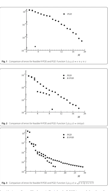
This section is devoted to the comparison of the practical performances of the feasible R-POD expansion. In particular, we confirm the exponential rate of convergence of the truncated POD expansion for the diffusion-reaction equation proved in section “Analysis of solutions of the reaction-diffusion”. We are also interested in comparing the rate of convergence of R-POD and PGD expansions, as the latter is particularly well suited to approximate multivariate functions. We have considered functions with high and low smoothness, as the smoothness plays a crucial role in the decreasing of the size of the modes in both expansions. In addition we have tested the ability of both representations to approximate functions that already have a separated tensor structure. For complete-ness we describe in the Appendix the application of the PGD expansion to approximate multivariate functions.
Multi-variate functions
In this test we apply the R-POD and the PGD to approximate multivariate functions. Actu-ally we consider tri-variate functions a generic test to determine the relative performances of both expansions. We have considered the following tests:
Case 1: Function with tensor structure.
S1(x, y, z)=x+y+z. (41)
Case 2: Function with non tensor structure.
S2(x, y, z)=sin(xyz). (42)
Case 3: Function with low regularity
S3(x, y, z)=
x+2y+z+4. (43)
The space domain is fixed to = X ×Y ×Z, with X = Y = Z =]−1,1[ and Gauss–Lobatto–Legendre quadrature is used (see [4]) with the polynomial degree equal toN=64. These formulas are used to evaluate the matrix representation of the operators
BandA.
0 4 8 12 16 20 M 10-12
10-8 10-4 100
PGD
Fig. 1 Comparison of errors for feasible R-POD and PGD. FunctionS1(x, y, z)=x+y+z
0 4 8 12 16 20 M 10-8
10-6 10-4
10-2 PGD R-POD
Fig. 2 Comparison of errors for feasible R-POD and PGD. FunctionS2(x, y, z)=sin(xyz)
0 5 10 15 20 25 30 M 10-8
10-6 10-4 10-2
100 PGD
R-POD
Fig. 3 Comparison of errors for feasible R-POD and PGD. FunctionS3(x, y, z)=√x+2y+z+4
require approximately the same number of modes to reach a moderate accuracy, however the R-POD is more efficient to reach high accuracy in all cases. Finally, that the error associated to the R-POD expansions is almost in all cases below the one associated to the PGD one for the same number of modes.
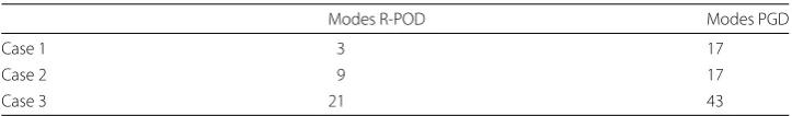
Table1displays the number of modes required by each expansion to reach the error below the threshold μ = 10−7. We observe that both expansions appear to converge for all cases considered, although in general both require a larger number of modes to approximate functions with lower smoothness. Also, that in all cases considered the R-POD requires less modes than the PGD.
Reaction-Diffusion equation
This part is devoted to determining the effective convergence rate of the R-POD approxi-mation of some solutions to the transient reaction-diffusion equation when parameterized by the diffusivity and reaction coefficients. We assess the exponential convergence rate and investigate the variation of this rate with respect to the setG=[γm,γM]×[αm,αM].
Test 1: Exponential convergence rate.
We consider the time-dependent reaction-diffusion equation in the domainQ=(0,1)× (0,1) and we select three possible pairs of source terms and initial conditions, given by
Data 1: f(t, x)=|x−t−0.3|, T0(x)=0,
Data 2: f(t, x)=0, T0(x)= |x−0.4|,
Data 3: f(t, x)=|x−t−0.3|, T0(x)= |x−0.4|.
These data have mild singularities, so the temperature solutions of (17), have a reduced regularity with respect toxandt, in particular fort = 0 for the two last data. The heat problem is discretized by an Euler scheme/Gauss–Lobatto–Legendre spectral method see [4] (the time step isδt=10−2and the polynomial degree isN =64).
Calculation for the matrix representations of the operators B andAare realized by means of accurate quadrature formulas. Indeed, various integrals (with respect to either
γ,αor (t, x)) are computed using Gauss-Lobatto quadrature formulas with high resolution in the corresponding intervals.
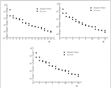
Figure 4 shows the convergence history of the R-POD expansion for the reaction-diffusion equation (40) in terms of the total number of modes in the expansion. We have considered the sets of diffusivitiesγ ∈[1,51], and reaction ratesα ∈[0,100]. The error is measured inL2(Q) norm. The numbers of secondary modesI
mhas been determined to
fit the testσ(Im+1)
m ≤ε=10−10. In practice a small amount of secondary modes (actually, Im 4) is needed to fit this test. The modes have been re-arranged in decreasing order
of the effective singular valuesτi(m)=σmσi(m)(denoted by asymbol). We observe that
theτi(m)indeed are good error estimators for this re-arranged expansion, as was argued in “Practical implementation” section.
Table 1 Comparison of feasible R-POD and PGD for trivariate functions
Modes R-POD Modes PGD
Case 1 3 17
Case 2 9 17
To assess the regularity of the eigenmodes associated to the conductivity parameterγ we choose to plot the three first corresponding to the most important singular values. The computational is made for case of Data 3. Based on Fig.5we clearly observe that these functions are regular. Same observation is made for the reaction parameter
Test 2: Dependence of the convergence rate with respect to the parameters range.
The dependence with respect to the ratio of diffusivitiesR=γM/γmof the exponential
convergence rate, stated by Theorem0.7, is illustrated in Fig.6. We depict the convergence
0 1 2 3 4 5 6 7 8 9 10 11 12 13 14 15
M
10-10 10-8 10-6 10-4 10-2 100
Singular Values L2-error
0 2 4 6 8 10 12 14
M
10-8 10-6 10-4 10-2 100
Singular Values L2-error
0 2 4 6 8 10 12 14
M
10-8 10-6 10-4 10-2 100
Singular Values L2-error
Fig. 4 Convergence history for POD expansion of the solution of the reaction-diffusion equation. Data 1 (top left), Data 2 (top right) and Data 3 (bottom)
0 10 20 30 40 50 Conductivity -1,0
-0,5 0,0
0,5 First mode
Second mode Third mode
0 2 4 6 8 10 12 14 M 10-6
10-4 10-2 100
R = 25 R = 64 R = 400
Fig. 6 Variation of the R-POD errors (in logarithmic scale) with respect to the ratioR=γM/γm, for fixed αm=0,αM=100. The variableMstands for the square root of the number of modes
history for Data 3, computed forR=25,64 and 400, in all cases with a fixed interval of reaction rates [αm,αM] = [0,100], with respect to the square root of the numbers of
modes,M=√L. We can point out that the convergence rate degrades asRincreases, in accordance with the fact that
ρ∗= γM2 γm −1
+1.
We observe some gap between the purely exponential decay of the error and the computed one, as the error curve in logarithmic coordinates appears to be a slightly concave curve instead of a straight line. This is consistent with the presence of the factorL1/4in estimate (37).
In Table2, we present the computed exponential convergence rateαc = 2 logρc, so
that theL2(G×Q) error, in terms of the number of modes after rearranging the RPOD series, is assumed to satisfy
e(L)=C e−αc √
L,
and the theoretical one given byα∗=2 logρ∗. The valueαcis calculated by exponential
regression. We indeed recover an exponential rate of convergence with respect to the square root of the number of modes, with an effective convergence rate larger than the theoretical one. We numerically state that the computed rate in all cases is larger than one (see Table2). We thus observe a kind of super-convergence effect.
We next test the dependence of the convergence rate with respect to the interval of reaction rates [α0,αM]. We show in Fig.7the convergence rates history corresponding
Table 2 Computed and theoretical convergence rates, for different values ofR=γM/γm
and fixedαm=0,αM=100(for Data 3)
R=γM/γm αc α∗
25 1.48 0.81
36 1.44 0.67
64 1.38 0.50
100 1.36 0.40
0 2 4 6 8 10 12 14 M 10-6
10-4 10-2 100
(0,10) (0,100) (0,500) (0,1000)
Fig. 7 Variation of the R-POD errors with respect to the reaction rateα. Thecurvescorrespond toα0=0, αM=10, 100, 500, 1000, withγm=1,γM=51 in all cases. The variableMstands for the square root of the number of modes
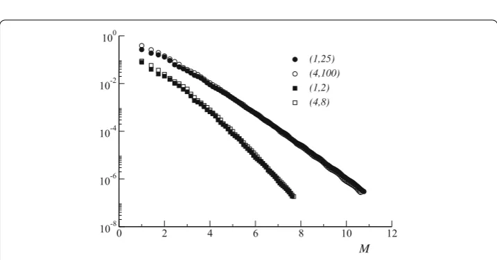
0 2 4 6 8 10 12 M 10-8
10-6 10-4 10-2 100
(1,25) (4,100) (1,2) (4,8)
Fig. 8 Analysis of dependence of the R-POD errors with respect to the ratioR=γM/γm. Thecurves correspond to the indicated pairs (γm,γM). The variableMstands for the square root of the number of modes
toαm = 0,αM = 10,100,500,1000 for fixedγm = 1,γM = 51. We observe a decrease
of the rate asαMincreases, that however appears to be uniformly bounded, in agreement
with estimate (37), where the dependence of the error bound with respect to [α0,αM] only
appears through the coefficientDρ.
The last numerical experiment studies wether the dependence of the exponential con-vergence on the diffusivities range [γm,γM] indeed takes place in terms of the ratio R=γM/γm. This is confirmed by the result plot in Fig.8, where we consider the couples
(γm,γM)=(1,2) and (4,8), corresponding toR=2, and (γm,γM)=(1,25) and (4,100),
corresponding toR=25, with fixedα0=0,αM =100.
Conclusion
expan-sions of the modes that appear in the expanexpan-sions at the previous level, to a given tolerance error. We have constructed a practical truncation error estimator by means of bounds for the singular values, which is used to recursively compute the expansion by the Power Iter-ate (PI) method. This allows to compute just the modes needed to attempt a given error threshold. We have proved the quasi-optimality of this RPOD expansion inL2, similar to that of the POD expansion.
We have proved the exponential rate of convergence of the RPOD expansion for the solution of the reaction-diffusion equation, based upon the analyticity of its solution with respect to those parameters.
We have finally performed some relevant numerical tests that on one hand show that the RPOD is more accurate than the PGD expansion for three-variate functions, and that on another hand confirm the exponential rate of convergence for the solution of the reaction-diffusion equation, presenting a good agreement with the qualitative and quantitative theoretical expectations.
Further extensive tests for more complex multivariate functions, in particular of practi-cal interest for engineering applications, are in progress and will appear in a forthcoming paper.
Authors’ contributions
MA, FBB and TCR participated to the development of the mathematical proves and the numerical investigations. They checked the results and wrote the manuscript. All authors read and approved the final manuscript.
Author details
1Bordeaux INP, I2M, (UMR CNRS 5295), 33607 Pessac, France ,2LMAC, EA 2222, Université de Technologie de Compiègne,
BP 20529, 60205 Compiègne Cedex, France,3I2M, IPB (UMR CNRS 5295), Université de Bordeaux, 33607 Pessac, France, 4Departamento EDAN & IMUS, Universidad de Sevilla, C/Tarfia, s/n, 41012 Sevilla, Spain.
Acknowledgements
None.
Competing interests
The authors declare that they have no competing interests.
Appendix: The PGD representation of multivariate functions
We describe in this section the procedure to calculate the PGD representation of a multi-variate functions. We focus on trimulti-variate functions for the sake of clarity. Its extension to general multivariate functions is straightforward.
The PGD approximation of a trivariate functionTsearches for an expansion of the form
T(x, y, z)=
m≥0
Xm(x)Ym(y)Zm(z), for (x, y, z)∈X×Y×Z. (44)
The leading termX0⊗Y0⊗Z0is initially computed by means of an adaptation of the
Power Iteration algorithm: Assume known an approximationX0(n−1)⊗Y0(n−1)⊗ Z0(n−1).
Step 1.FindZ0(n)∈L2(Z) such that for allZ∗∈L2(Z),
X0(n−1)⊗Y0(n−1)⊗Z0(n)−T, X0(n−1)⊗Y0(n−1)⊗ Z∗
L2(X×Y×Z)=0. (45) Step 2.Find ˜X0(n)∈L2(X) such that for allX∗∈L2(X),
˜
X0(n)⊗Y0(n−1)⊗ Z0(n)−T, X∗⊗Y0(n−1)⊗Z0(n)
L2(X×Y×Z)=0. (46) Set
X0(n)= X˜ (n) 0 X˜(n)
Step 3.Find ˜Y0(n)∈L2(Y) such that for allY∗∈L2(Y),
X0(n)⊗Y˜0(n)⊗ Z0(n)−T, X0(n)⊗Y∗⊗ Z0(n)
L2(X×Y×Z)=0. (47) Set
Y0(n)= Y˜ (n) 0 Y˜(n)
0 L2(Y) .
The procedure is to be iterated until the error eventually is below a given tolerance. TheMth modeXM⊗YM⊗ZMis computed in the same way, by replacing the function T by the residualT−TˆM−1, where now
ˆ
TM−1(x, y, z)=
0≤m≤M−1
Xm(x)Ym(y)Zm(z), for (x, y, z)∈X×Y×Z. (48)
In this way, the residualT−TˆMis orthogonal toSpan(XM⊗YM⊗ZM).
There is no proof, up to the knowledge of the authors, that the PGD expansion (44) exists for functionsT ∈L2(X×Y×Z) or perhaps with additional regularity, nor that the alternate Power Iteration process (45)–(47) converges. There is a proof, however, that for general functions depending on three or more parameters, there does not exist optimal sub-spaces of finite dimension 3 or larger, that satisfy the optimal approximation property set by Theorem0.2(see [9]).
Received: 24 November 2015 Accepted: 11 February 2016
References
1. Azaïez M, Belgacem Ben F. Karhunen-Loève’s truncation error for bivariate functions. Comput Methods Appl Mech Eng. 2015;290:57–72.
2. Azaiez M, Ben Belgacem F and Chacón Rebollo T. Error bounds for POD expansions of parameterized transient temperatures. Submitted to Comp. Methods App. Mech. Eng.
3. Berkoz G, Holmes P, Lumley JL. The proper orthogonal decomposition in the analysis of turbulent flows. Annu Rev Fluids Mech. 1993;25:539–75.
4. Bernardi C, Maday Y. Approximations spectrales de problèmes aux limites elliptiques, Mathématiques et applications. Berlin: Springer; 1992.
5. Chinesta F, Keunings R, Leygue A. The Proper Generalized Decomposition for Advanced Numerical Simulations: A Primer. New York: Springer Publishing Company, Incorporated; 2013.
6. Chinesta F, Ladevèse P, Cueto E. A Short Review on Model Order Reduction Based on Proper Generalized Decompo-sition. Arch Comput Methods Eng. 2011;18:395–404.
7. De Lathauwer L, De Moor B, Vandewalle J. A multilinear singular value decomposition. SIAM J Matr Anal Appl. 2000;21(4):12531278.
8. De Lathauwer L, De Moor B, Vandewalle J. On the Best Rank-One and Rank-R1; R2;.; RN Approximation of Higher Order Tensors. SIAM J Matr Anal Appl. 2000;21(4):13241342.
9. De Silva V, Lim LH. Tensor rank and the ill posedness of the best low-rank approximation problem. SIAM J Matrix Anal Appl. 2008;20(3):1084–127.
10. Diestel J and Uhl. Vector measures. AMS J J; 1977.
11. Epureanu BI, Tang LS, Paidoussis MP. Coherent structures and their influence on the dynamics of aeroelastic panels. Int J Non-Linear Mech. 2004;39:977–91.
12. Ghanem R and Spanos P. Stochastic finite elements: a spectral approach. Springer-Verlag; 1991. 13. Golub GH, Van Loan CF. Matrix Computations. 3rd ed. Baltimore: The Johns Hopkins University Press; 1996. 14. Heyberger C, Boucard PA, Néron D. A rational strategy for the resolution of parametrized problems in the PGD
framework. Comp Meth Appl Mech Eng. 2013;259:40–9.
15. Heyberger C, Boucard PA, Néron D. Multiparametric Analysis within the Proper Generalized Decomposition Frame-work. Comput Mech. 2012;49(3):277–89.
16. Holmes P, Lumley JL, Berkooz G. Coherent Structures, Synamical Systems and Symmetry, Cambridge Monographs on Mechanis. Cambridge: Cambridge University Press; 1996.
17. Hotelling H. Analysis of a complex of statistical variables into principal componentse. J Educ Psychol. 1933;24:417–41. 18. Jolliffe IT. Principal Component Analysis. Springer; 1986.
19. Little G, Reade JB. Eigenvalues of analytic kernels. SIAM J Math Anal. 1984;15:133–6. 20. Loève MM. Probability Theory. Princeton: Van Nostrand; 1988.
21. Lorente LS, Vega JM, Velazquez A. Generation of Aerodynamic Databases Using High-Order Singular Value Decom-position. J Aircraft. 2008;45(5):1779–88.
23. Nouy A. A generalized spectral decomposition technique to solve a class of linear stochastic partial differential equations. Comput Meth Appl Mech Eng. 2007;196:4521–37.
24. Pearson K. On lines and planes of closest fit system of points in space. Philo Mag J Sci. 1901;2:559–72.
25. Trefethen LN. Approximation theory and approximation practice. Software, Environments, and Tools. Philadel-phia: Society for Industrial and Applied Mathematics (SIAM); 2013.
26. Willcox K, Peraire J. Balanced Model Reduction via the Proper Orthogonal Decomposition. AIAA. 2002;40:2323–30. 27. Yano M. A Space-Time Petrov-Galerkin Certified Reduced Basis Method: Application to the Boussinesq Equations.