The Thirty-Third AAAI Conference on Artificial Intelligence (AAAI-19)
Traffic Updates: Saying a Lot While Revealing a Little
John Krumm, Eric Horvitz
Microsoft Research Redmond, Washington USA[email protected], [email protected]
Abstract
Taking speed reports from vehicles is a proven, inexpensive way to infer traffic conditions. However, due to concerns about privacy and bandwidth, not every vehicle occupant may want to transmit data about their location and speed in real time. We show how to drastically reduce the number of trans-missions in two ways, both based on a Markov random field for modeling traffic speed and flow. First, we show that a only a small number of vehicles need to report from each location. We give a simple, probabilistic method that lets a group of ve-hicles decide on which subset will transmit a report, preserv-ing privacy by coordinatpreserv-ing without any communication. The second approach computes the potential value of any loca-tion’s speed report, emphasizing those reports that will most affect the overall speed inferences, and omitting those that contribute little value. Both methods significantly reduce the amount of communication necessary for accurate speed infer-ences on a road network.
1
Introduction
Accurate traffic speed information is vital for computing ef-ficient routes for vehicles on roads. Dedicated road sensors, such as embedded induction loops, are expensive to install and maintain. An obvious alternative is to use the mobile phones of vehicle occupants to sense and report speeds to a central server. As of early 2018, 95% of Americans owned a cellphone of some kind, and 77% owned a smartphone (Cen-ter 2018). Both fractions are rising. As an example, Waze gathers GPS data from its users at a rate of one reading per second to compute road speeds to use for routing (Parmy Ol-son 2014). This location data not only uses bandwidth, but it is vulnerable to privacy attacks. In fact, researchers were able to create fake Waze accounts that allowed them to track Waze users (Wang et al. 2018), a vulnerability that was patched by Waze (Waze 2016). Even coordinating among vehicles with vehicle-to-vehicle communication has nega-tive privacy implications (Williams 2017).
Problems with bandwidth and privacy can be fixed with advanced compression (Lelewer and Hirschberg 1987) and location privacy techniques (Krumm 2009), respectively. However, another solution is to transmit less data. This paper introduces two techniques to reduce the number of revealing
Copyright c⃝2019, Association for the Advancement of Artificial Intelligence (www.aaai.org). All rights reserved.
Figure 1: The white circles show 109 traffic measurement stations around central Los Angeles, California, USA. The black lines show which stations were connected in the Markov random field.
transmissions required to maintain accurate inferences about traffic speeds. Both approaches are based on a Markov ran-dom field (MRF) that models varying quantities of vehicle speed report data as well as the observed correlations be-tween traffic conditions on different parts of the road net-work. Using this model, we show that a small number of speed reports can be combined to infer traffic conditions on all the roads in the network.
maintaining approximately the desired number of vehicle re-ports.
Our second technique is sensitive to the fact that not all road segments need a speed measurement. In fact, if traffic is moving normally, no reports are necessary. We formal-ize this with a value-of-information analysis. Each vehicle runs a local version of the MRF to assess approximately how much its own speed report would affect traffic inferences on the whole road network. Reports that would have a larger effect on the network are prioritized over those that would have little or no effect.
Next we describe the traffic data and MRF model that we used for our experiments.
2
Traffic Data
Our experimental data consists of freeway speeds and flows from the state of California in the USA. Traffic on roads is often characterized by its speed and flow, where flow in-dicates the number of vehicles passing a certain point in a given amount of time. Such data is available free via the California Performance Measurement System (PeMS), which provides a wide variety of real-time and historical data for freeways in California (California Department of Transportation (Caltrans) 2018). PeMS includes traffic data collected from over 35,000 traffic detectors that report every 30 seconds. The main type of detector is inductive loops, but there are also side-fire radars and magnetometers. PeMS ag-gregates this data into reports from discretely located mea-surement stations, each of which covers all freeway lanes in the same direction. For instance, one station may pertain to all northbound lanes at a particular location on Interstate 5. PeMS reports the data at five-minute intervals, giving the mean speed and count of vehicles per five minutes (flow) at each station. We maintain this five-minute time discretiza-tion throughout our analysis.
For our experiments, we chose data from 109 different freeway measurement stations inside in a 3.1 mile (5 kilo-meter) radius around the center of Los Angeles, California, USA, shown in Figure 1. Figure 2 shows the speed and flow averaged over all 109 stations for one day. In the subsequent sections of this paper, we refer to these measurement stations as simply ”stations”. We used data from the first six months of 2017 for training and the last three months for testing. We used months 7-9 for value-of-information training described in Section 7.
Next we describe a method to infer speeds at all the sta-tions based on noisy speed reports from only a subset of the stations.
3
Markov Random Field for Traffic
We develop a Markov random field (MRF) for statistical modeling of macroscopic traffic speeds and flows. This model is particularly well-suited to our task of reducing the number of of traffic speed reports, because it propagates measurements from a subset of the stations to make infer-ences for all the stations
3.1
Previous Work
Previous traffic models have included the vector autore-gressive (VAR) model of Liu et al., which models speeds on a particular road segment as a weighted, linear sum of speeds on other road segments (Liu et al. 2016). Hongzi Zhu et al. use a multi-channel singular spectrum analysis (MSSA) model to infer traffic speeds despite noise and miss-ing values (Zhu et al. 2009). In the work by Yanmin Zhu et al., the authors find correlations between traffic on differ-ent roads through principal compondiffer-ent analysis (PCA) (Zhu et al. 2013). JamBayes uses a Bayesian network to in-fer and predict traffic based on several features like cur-rent traffic, road incidents, weather, holidays, and planned events (Horvitz et al. 2012). Zhang et al. demonstrate a deep, residual network to predict crowd flows, including inputs such as weather (Zhang, Zheng, and Qi 2017). There are also microscopic traffic flow models, often based on physics (e.g. (Nagatani 2002)), but our interest here is in a more data-driven model that can be used to understand and exploit the value of small amounts of traffic data for making network-wide inferences.
An MRF model has been applied to traffic before, e.g. for modeling images of vehicles at intersections (Kamijo et al. 2000) and for using Twitter to sense traffic (Chen, Chen, and Qian 2014). The most relevant previous MRF work is that of Kataoka et al. (Kataoka et al. 2014). Their MRF helps fill in missing traffic data based on sensed data at other locations. The distributions in their MRF are parametric, while we use nonparametric probability distributions learned from histor-ical data. Our nonparametric formulation has the advantage of representing arbitrary relationships between traffic con-ditions on different roads. This more flexible representation allows us to model both the speed and flow, rather than just density. Furthermore, we use multiple MRFs targeted at dif-ferent days of the week and times of day, while Kataoka et al’s approach uses a single MRF for all time. Hu et al. also use an MRF for traffic estimation, specifically looking for certain ”seed roads” which are most indicative of traffic conditions on other roads (Hu et al. 2016). Their model pro-duces a binary indicator that shows if the traffic is moving faster or slower than average.
The main innovation of our MRF model, however, is how we use it. The VAR, MSSA, PCA, and MRF models ref-erenced above are mostly aimed at filling in missing traffic values by exploiting correlations discovered in historic traf-fic data. In contrast, our work aims at using a small number of traffic reports, including possibly zero, while still main-taining accuracy.
3.2
Markov Random Field
Our MRF model represents each traffic variable (i.e. speed and flow) in a road network as a connected node in a graph-ical model. For each of the N measurement stations, the scalar variablessi andfi,i = 1. . . N, represent the mean
Figure 2: This shows the mean speed and flow over all 109 measurement stations around downtown Los Angeles, California, USA on 19 April 2017.
the hat indicates this is a noisy measurement that likely de-viates from the actual value. It would be difficult for a single probe vehicle to measure flow, so we assume a vehicle can only report speed.
The MRF depends on so-called compatibility functions between variables. These are often expressed as pairwise joint probability functions between pairs of variables. We have the following discrete, joint PDFs to represent relation-ships among the actual speeds, actuals flows, and measured speeds:
• Psi,sj(si, sj)is the relationship between speeds at mea-surement stations i and j. The most useful of these is when i ̸= j, which represents the joint PDF of speeds at two different stations.
• Psi,fi(si, fi)is the relationship between speed and flow at stationi. Although there are approximations of this re-lationship (e.g. (Akcelik 1996)), we learn the rere-lationship from the data.
• Psi,sˆi(si,sˆi) is the relationship between the actual and measured speeds at stationi. These are different due to measurement noise of the vehicle. Since ˆsi is a given
measurement, we abbreviate this PDF with the simpler
Psi(si)and call it a measurement distribution.
Graphically, we can think of the MRF as an undirected graph with a node for each variable and an edge for each joint PDF, as in Figure 3. Seeing it this way gives rise to ideas for other topologies, such as introducing joint PDFs between the roads’ flow variables or between one road’s speed an another road’s flow. While the MRF offers this flex-ibility, we found the given topology to be adequate for our purposes.
Adopting the development in (Yedidia, Freeman, and Weiss 2003), the overall joint probability of the speeds,
Figure 3: This is a graphical representation of the variables for a road network with three measurement stations. The measured variables are associated with the filled-in circles, and the unknowns are in the white circles. Each edge is rep-resented by a joint PDF.
flows, and measured speeds of the measurement stations is
P({
s}
,{
f}
,{
ˆ
s}
) = ∏
(ij)
Psi,sj(si, sj)×
∏
i
Psi,fi(si, fi)×
∏
i
Psi,sˆi(si,sˆi)
(1)
Here{s}
is the set of all speeds, and similarly for{f}
. The term {ˆs}is the set of measured speeds. The notation(ij)
to find values ofsandf that maximize the joint probability in Equation (1). This gives the inferred speeds and flows that we want.
3.3
Loopy Belief Propagation
The joint distribution in Equation 1 is difficult to optimize in a straightforward way, given that we have over 100 mea-surement stations, each with its own speedsi, flowfi, and
a potential measurementˆsi. To make this easier, we begin
with a slight reformulation of Equation 1 which does not include the inviolate speed measurementssˆi, because they
do not change. This means the joint PDFs for measurements become simply one-dimensional PDFs over the speed val-ues. That is,Psi,ˆsi(si,sˆi) becomes simply Psi(si), which gives the distribution of speeds based on a tangible speed measurement at stationi. The joint probability with only the unknown variables is
P({
s}
,{
f}
) =∏
(ij)
Psi,sj(si, sj)
∏
i
Psi,fi(si, fi)Psi(si)
(2) Belief propagation (BP) is an algorithm that can find thea posterioridistributions, or beliefs, of all the unknown vari-ables in a joint PDF like Equation 2 (Yedidia, Freeman, and Weiss 2003). That it finds the distributions, rather than simply the maximuma posteriori, is advantageous, because the distributions represent the uncertainty of the inferences. BP proceeds by passing messages along the edges of the joint PDF graph. The details of the messages are available in many tutorials, including (Yedidia, Freeman, and Weiss 2003). Each node receives messages from all its connected nodes. A received message is a distribution over the recipi-ent’s domain of possible values that gives the sender’s belief of what the recipient’s state should be. The recipient com-bines the messages to form itsa posterioridistribution. In a graph without loops, these messages need to be passed only once to provably converge to the exacta posteriori distribu-tions.
In our problem, the graph has loops, as shown in the ex-ample graph in Figure 3. Fortunately, repeatedly sending up-dated messages, i.e. loopy BP, often works in these cases, with thea posterioridistributions converging after enough rounds of message-passing. We stopped our program’s sage passing after the mean absolute difference in each sage over time dropped below 0.1 or if the number of mes-saging iterations exceeded 100. For our experiments, loopy BP always converged. The result of loopy BP is a PDF of the inferred values of speed and flow at each station. We used the mode of the PDFs to extract inferred scalars to compare to ground truth. In Section 7 we need individual vehicles to run loopy BP. On a conventional desktop PC, our custom BP code converged in an average of 20 milliseconds, so it is feasible to run in a vehicle.
3.4
Joint Probabilities for Road Speed and Flow
The joint probabilities Psi,sj(si, sj) andPsi,fi(si, fi) de-scribe how speeds and flows on the road network vary with each other, and they come from temporally co-occurring
pairs of speed and flow in our six months of freeway train-ing data. We computed these joint probabilities in the classic way by normalizing frequency counts of discretized pairs of measurements. For all our MRF inferences, we discretized speeds into 5 mph bins, and we discretized flows into 25 vehicles/5 minutes bins. For the speed-flow probabilities
Psi,fi(si, fi), we computed a joint PDF for each measure-ment station. The speed-speed PDFs, Psi,sj(si, sj), relate speeds between pairs of measurement stations. To limit the complexity of our MRF, we only computed a speed-speed PDF between stationiandjif stationj was one of station
i’s ten nearest neighbors or vice-versa, using the great circle distance. This is based on an assumption that traffic effects are mostly local, which was justified by the overall accuracy of our model. For pairs of measurement stations not in each other’s set of nearest neighbors, there was no edge between them in the MRF. The black lines in Figures 1 and 3 show which pairs of stations were connected by a joint PDF.
To account for possibly different relationships between traffic on different days of the week and at different times of day, we split a canonical week into five-minute intervals and computed a separate set of joint PDFs, and thus a separate MRF, for each five-minute interval. For example, we had one MRF for Mondays from 8:00 a.m. - 8:05 a.m. and a different MRF for Saturdays from 10:45 p.m. - 10:50 p.m., giving a total of 2016 MRFs to cover one representative week.
3.5
Probabilities for Measured Speed
Practically, representing the uncertainty in speed measure-ments is important in that it allows the MRF to settle on speed inferences that are a compromise between the speed measurements and the joint PDFs. The joint PDFs serve as a sort of prior on speeds, flows, and their relationships. If measured speeds were injected into the MRF with no uncer-tainty, loopy belief propagation would simply converge to the measured speeds, ignoring the joint PDFs.
One important representational advantage of the MRF be-comes apparent with the measured speed distributions. In our algorithm for selecting which vehicles should report their speeds, some measurement stations have no associated speed report. We represent thisPsi(si)as simply a uniform speed distribution over the range zero to the maximum speed observed at the station during training. This lets the asso-ciated node float based solely on messages passed in from its connected nodes. One extreme we explore in our experi-ments is to set allspeed reports to uniform and let the entire MRF float to a set of inferences which are essentially inde-pendent of any measurements.
4
Probabilistic Speed Reports from GPS
In our scenario, a subset of vehicles on the road report their speeds to a central server, which in turn makes network-wide speed and flow estimates using an MRF. This section describes how we model the inherent noise in these speed reports, due to both the natural variation in speed among a group of vehicles and due to measurement noise.we need to model speed reports from individual vehicles. Here we seek to derive a probability distribution that de-scribes these invidual reports. We model the variation from two sources: the natural differences between vehicle speeds traveling on a road and the noise due to GPS measurement error.
The first source of speed variation is the natural differ-ences of speeds among vehicles traversing the same road segment. This variation has been studied for its effects on crashes (Kockelman and Ma 2010) and audible noise (Ian-none, Guarnaccia, and Quartieri 2013). While our traffic data gives mean speeds, we want to assess the effect of speed reports from different vehicles passing the same mea-surement point on the road, whose speeds will inevitably be different. In (Iannone, Guarnaccia, and Quartieri 2013), Iannone et al. review work on speed variation, noting that the dominant model is a simple Gaussian probability dis-tribution, which works best for free-flowing traffic. (Ian-none, Guarnaccia, and Quartieri 2013) says that the stan-dard deviation σsnatural normally varies between 3.1 and 12.5 mph. Using PeMS data sampled at 30 seconds and ag-gregated over 5-minute periods, we found a meanσsnatural of 5.3 mph. Using regression, we also found that the road’s mean speed and flow were poor predictors ofσsnatural, so we chose to use this constant value throughout our analy-sis instead of trying to infer it based on road parameters or traffic measurements.
The second source of speed variation is measurement noise. We assume that vehicles measure their speed using pairs of location measurements from their onboard GPS sen-sors 1. Using the common Gaussian noise assumption for GPS (Diggelen 2007), a location measurement vector is dis-tributed as xi ∼ N
(
[xi, yi]T, σg2I )
. We approximate the standard deviation of GPS asσg= 3 meters. Taking the
tor difference of two measurements gives the velocity vec-tor:
vi=
µi−µi−1
∆ti
where ∆ti = ti − ti−1, µi = [xi, yi]T, and µi−1 =
[xi−1, yi−1]T. For our simulation, we take∆ti=2 seconds.
If the two location measurements are independent, their variances will add, and the two-dimensional distribution of the velocity vector will be:
vi∼ N (µ
i−µi−1
∆ti
,2
( σ
l
∆ti )2
I
)
whereIis the 2x2 identity matrix.
We now have a distribution for the velocity vector, but we are ultimately interested in the distribution for scalar speed, which is the magnitude of velocity. For the case of a bivariate normal with a diagonal covariance matrix, the distribution of the magnitude follows a Rician distribution (Rice 1945):
1
We could also use a speed measurement from the vehicle’s speedometer. However, we are assuming that a cell phone in the vehicle is used for both communication and speed measurements, eliminating the need for the phone to interface with the vehicle’s speedometer.
||vi|| ∼Rice (||µ
i−µi−1||
∆ti
,
√
2σl
∆ti )
.
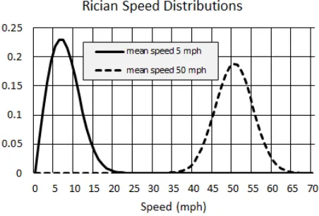
Two example Rician speed distributions are shown in Fig-ure 4. When the Rician’s mean is sufficiently larger than its standard deviation, the Rician can be approximated by a Gaussian with the same mean and standard deviation. Thus, we model the measurement noise as a Gaussian with standard deviation σsmeasurement =
√
2σl
∆ti = 2.12 m/s=
4.74mph.
Figure 4: These are two Rician speed distributionsPsi(si), assuming GPS precision ofσg = 3 meters and a GPS
sam-pling interval of∆ti=2 seconds.
With two additive sources of Gaussian noise, the vari-ances add to give a speed report distribution of S ∼
N(µs, σs2), whereµsis the mean speed from our 5-minute
traffic data, and
σ2s=σ 2
snatural+σ
2
smeasurement. (3)
We use this value of σ2
s for our experimental simulations
and for assigning uncertainty to speed measurements for our MRF.
5
Markov Random Field Baseline
In this section we give a baseline scenario to explore how decreasing the number of speed reports affects the accuracy of our traffic inferences. We call this a baseline, because we modify this scenario in subsequent sections for more effi-ciency and privacy.5.1
Reporting Structure
We assume the central server will receive the vehicle speed reports. For those reports coming from the same station, the server will compute the mean of the reported speeds. The distribution of the mean ofnreports, where each report is distributed asN(µs, σ2s), isN(µs, σ2s/n), meaning
the precision is increased. Note thatσsrepresents the speed
uncertainty from Equation 3, due to both measurement noise and the natural variation in speeds among a group of vehi-cles on the same road.
5.2
Experiments
As mentioned above, we used PeMS data from the first six months of 2017 to compute the joint PDFs necessary for the MRF. This is the training phase. We used data from the last three months of 2017 for testing. Our results show the in-ference error over 10,000 independent tests. Each test con-sists of first choosing a random 5-minute reporting interval in our test data. Inside each test, we randomly shuffle the list of measurement stations and then increment from 0 to all 109 stations, gradually including speed reports from more stations. For each tested subset of stations, we compute the root mean square (RMS) speed error between the ground truth and the mode of the inferred speed PDF at each station. We also computed a demand-weighted RMS error based on the actual vehicle flow at each station. Specifically, if the speed error at a station is∆si, then the demand-weighted
error is∆sifi, where fi is the flow in number of vehicles
per five minutes. The total demand-weighted RMS error,
√ 1 N
∑ N∆s
2
ifi2, accounts for the actual number of vehicles
that would experience the speed error, placing less empha-sis on lightly-traveled roads and more on heavily-traveled roads.
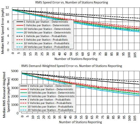
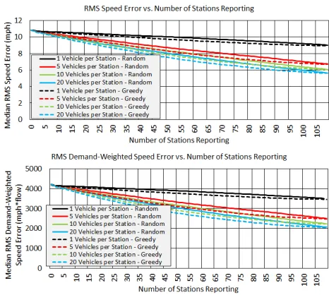
The accuracy results are shown in Figure 7. The horizon-tal axis represents an increasing number of randomly shuf-fled reporting stations. The solid lines in both plots show how the median RMS speed error and median RMS demand-weighted speed error both fall with more stations reporting, as expected. Here the medians are taken over the 10,000 random tests. It is also apparent that increasing the num-ber of vehicles reporting from each station reduces error. The topmost solid curve in both plots shows the error with only one vehicle reporting from each station, and the other curves show how the error decreases withn = 5,10, and
20vehicles reporting. This decrease in error is because the precision of the speed reports changes as σ2
s/n. We note
that demand-weighted RMS error has the awkward units of (mph)*(vehicles/(5 minutes)). For the remainder of the paper, we will abbreviate (vehicles/(5 minutes)) as simply ”flow”, meaning that demand-weighted RMS error has units mph*flow.
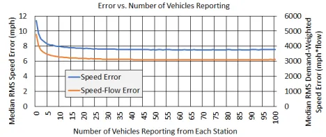
Looking more closely at error vs. the number of vehi-cles reporting, Figure 5 shows how speed error and demand-weighted speed error both drop with more vehicles reporting if a random subset of 54 stations (about half) report. Beyond reports from about 20 vehicles, there is not much to gain in terms of error reduction. Because of this, for the remainder of this paper, we give results forn= 1,5,10, and20 vehi-cles reporting.
We can quantify the reduction in speed reports. The mean traffic flow over our 3-month test period was 240.4 vehi-cles/5 minutes at each measurement station. If all vehicles reported their speeds every 5 minutes at all 109 stations, the total number of reports would be109×240.4 = 26,204
reports every 5 minutes. If only M stations report (M ≤
N = 109) with onlynvehicles per station, then the total number of reports would be M n every five minutes. The plots in Figure 7 show that inference error drops steadily with increasing number of stations reporting, so we will have
M = 109to represent all stations reporting. However, the plots show that, say,n = 20vehicles reporting from each station appears to be approaching the minimum error value. With these settings ofM andn, the number of reports is re-duced by a factor of(109×20)/(109×240.4) = 0.083. Thus the overall accuracy of the system is maintained with only about 8% of all the vehicles reporting, representing an order of magnitude reduction in privacy-compromising communi-cation and bandwidth.
This baseline depends on some sort of vehicle-to-vehicle coordination such that only a predefined number of vehicles report their speed from every station. The next section ex-plores a method to eliminate the necessity of communicating to coordinate.
Figure 5: As more vehicles report their speeds, there are di-minishing returns beyond about 20 vehicles. This plot shows computed errors for reports from random subsets of 54 sta-tions out of all 109.
6
Coordinating Multiple Vehicle Reports
Without Communication
In our scenario, vehicles each make independent decisions about whether or not to report their speed, and these deci-sions are renewed every five minutes. One way to reduce the number of reports is to send them only when the measured speed is unusually above or below expectations. We detail this idea in Section 7. Another way to reduce the number of reports is to have only a few vehicles on each road seg-ment report their speed, as described in the previous section. Here we look at how to select a subset of vehicles to report without any communication from them.
6.1
Probabilistic Coordination
coordinate via wireless, this represents a potential privacy leak, and such coordination has yet to be standardized. In-stead, we demonstrate an example of ”coordination without communication” (Fenster, Kraus, and Rosenschein 1995). If a vehicle decides that a report would be useful, we have it re-port with a probabilitypr, regardless of what other vehicles
might be doing.
In a five-minute period, there are f vehicles passing a point on a road, where f indicates flow/5 minutes.2 With
f vehicles each making a report with probability pr, the
expected number of reports isprf, and the distribution of
the number of vehicle reports is binomial. In particular, the probability of getting at least one report ispone= 1−(1−
pr)f, shown in Figure 6. A system operator could setprsuch
thatponealways maintains some minimum value.
Figure 6: This is the probability of a group of vehicles send-ing at least one report for different group sizes and reportsend-ing probabilities.
A suitable scheme for probabilistic coordination would have a system-wide minimum threshold on the expected number of vehicle reports,E[n], from every station. With
E[n] =prf, each vehicle could compute its own
probabil-ity of reporting aspr = E[n]/f. Each vehicle would
gen-erate a uniformly distributed random numberu∈[0,1]and transmit its speed to the central server ifu≤pr.
The probabilitypr depends on the flow f, which is not
easily measurable from a moving vehicle. However, for each stationi, the vehicle can estimate the flow distribution from the joint PDFPsifi(si, fi). With the vehicle measur-ing its own speed ofsˆi, the flow distribution is Pfi(fi) =
Psifi(ˆsi, fi), and the scalar flow estimate is taken as the mean or mode of this distribution. We used the mode in our experiments.
6.2
Experiments
Our experiments for this scenario are designed to investi-gate the effect of multiple vehicle reports from each station
2
We could model a smaller pool of potential vehicle reports by reducing the number of potential participants toαf, with0< α≤
1, but we will assume full participation withα= 1for our analysis.
and to understand the efficacy of coordinating reports prob-abilistically without communication among vehicles. Our baseline is the MRF model from Section 5, where we ex-amined the effect of incrementally increasing the number of stations reporting and where each station has speed reports fromn= 1,5,10, and20vehicles. This baseline is shown as the solid curves in Figure 7.
Figure 7: The solid lines show how the speed error (top plot) and demand-weighted speed error (bottom plot) change with the number of stations reporting and the number of vehicles reporting from each station. The corresponding dashed lines show the same errors when all the vehicles coordinate prob-abilistically without any communication from them.
Using the probabilistic reporting technique from above, Figure 7 shows that it works almost as well as its determin-istic counterpart. In this figure, the dashed lines represent the probabilistic technique, and their colors colors correspond to the deterministic technique with the same target number of vehicles reporting.
Summarizing, Section 5 shows that only a relatively small subset of vehicles need to report from each station, and this section shows that the subset can be self-selected with no need for communication, enhancing privacy and reducing bandwidth. Next we describe a technique to prioritize which stations should report, which can further decrease the num-ber of speed reports while still maintaining accuracy.
7
Prioritizing Reports with Value of
Information
in cooperation with the central server, vehicles would either transmit their speed reports or not, based on their local self-assessments. When some vehicles choose not to report, this further reduces the communication necessary for maintain-ing accurate traffic inferences.
7.1
Defining Value of Information
We define the value of information (V OI) of a vehicle speed report as the RMS of the reduction in demand-weighted speed error over the road network. To define this precisely, we begin by introducing a functions′i(S)which represents the MRF’s estimate of the speed at stationibased on a set of speed reportsSfrom a subset of stations in the network. The expressions′i(∅)is the MRF estimate of ofsibased on
no speed reports.
Ideally we would compute a quantity like Equation 4, which reflects the RMS error between the nominally ex-pected speeds,s′j(∅), and the actual speedssj, weighted by
the actual flowsfj:
V OI =
√
1
N
N ∑
j=1
f2
j(s′j(∅)−sj)2 (4)
This quantity gives the error between the ground truth speeds and the nominally expected speeds from the MRF if there were no speed reports, assuming ground truth speeds and flows are available. However, an independently operat-ing vehicle does not have access to the actual speeds and flows, so it must estimateV OI based on what it can mea-sure.
7.2
Estimating Value of Information
Our algorithm depends on each vehicle being able to assess the V OI of its own speed report. Because theV OI from Equation 4 depends on ground truth values of speed and flow (sj andfj) over the whole network, individual
vehi-cles could not computeV OI independently. However, they can estimateV OIby inferring the speeds and flows over the network using an MRF. Specifically, a vehicle at stationican use its own measured speedsˆito compute an estimate of any
speed and flow in the network withs′
j({ˆsi})andfj′({ˆsi}),
respectively. Using these self-estimated values of speed and flow, the vehicle can then estimate the network-wideV OI
of its own speed report as
V OI′(ˆsi) = √
1
N
N ∑
j=1
(fj′({sˆi})2(s′j(∅)−s′j({sˆi})2 (5)
V OI′(ˆsi)can be considered as an estimate of the amount of
surprise that would be caused by transmitting speed report
ˆ
si to the central server. If the estimatedV OI is high, then
the system would be be surprised by the report compared to its nominal traffic conditions.
The system-wideV OIestimate in Equation 5 is perched tenuously on a single speed measurement. In order to boost accuracy, we introduce a machine-learned regression model that uses two numerical features to make a revised estimate
ofV OI, calledV OI′′. The first of these features is the orig-inal estimatedV OI′( ˆsi). The second feature is the elapsed
time from the start of the most recent Monday, called∆tM.
This helps contextualize the originalV OIestimate in time, accounting for the possibility that traffic surprises may be more or less important at certain times of the week. Thus we have a finalV OI estimate asV OI′′( ˆsi,∆tM). We
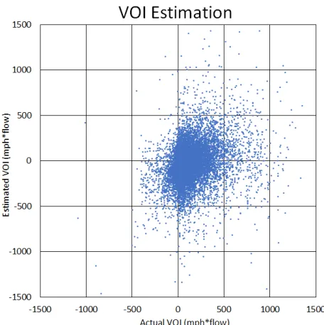
imple-mented this regression as a forest of boosted decision trees, and we learned one model for each of the 109 measurement stations using months 7-9 of our PeMS data for training. The median absoluteV OI prediction error over all 109 stations was 0.058 mph*flow, based on an 80/20 train/test split of the PeMS data from months 7-9. Figure 8 shows a plot of the ground truth and estimated VOI from our models.
Figure 8: These are the actual and estimated VOI values from our learned regression model. The median absolute er-ror was 0.058 mph*flow.
7.3
Experiments
One way to use the V OI estimates is to eliminate speed reports that fall below a preset V OI threshold. We com-puted the accuracy rate for the inferred V OI values
V OI′′( ˆsi,∆tM). An accurate inference is when the inferred
V OI says an instance is below a givenV OIthreshold and the V OI actually is below the threshold. Figure 9 shows this test accuracy rate using the same 80/20 train/test split as above. The rate is consistently above 0.965. This plot also shows that over 90% of the actual V OI values are below 1.0 mph*flow. This means that a large majority of speed re-ports have little value and that ourV OIinference procedure can accurately identify these useless reports.
Figure 9: TheV OIinference is accurate at finding speed re-ports that are below a given VOI threshold (red curve). Also, a large majority of potential speed reports have a very low
V OI(blue curve). TheV OIinferences can accurately iden-tify these useless reports. Note that the vertical axis starts at 0.90.
data we used for testing in Section 6. For each randomly cho-sen date and time in the test set, we first incremented through a randomly shuffled list of stations. This baseline shows how the RMS speed error and demand-weighted speed error de-crease as more stations report. To test theV OIapproach, we usedV OI′′( ˆsi,∆tM)to estimate theV OIof a report from
each station. The stations then reported in descending order of estimatedV OI, which was designed to test the effect of processing the most important reports earlier. In a real sys-tem, we would implement this greedy approach in a way that does not require vehicles to transmit anything until their re-port was needed. For instance, the central server might send out a decreasing sequence ofV OI thresholds, and vehicles would respond with a report when their estimatedV OI ex-ceeded the broadcast threshold.
The results of these tests are shown in Figure 10. The
V OI approach gives consistently lower RMS errors than the random approach, validating the effectiveness of this method. Although the improvement seems small in Fig-ure 10, looking at the results another way shows a relatively dramatic improvement. In Figure 11, the horizontal axis is the number of station reports from theV OI method. The vertical axis shows how many more reports the random ap-proach would need to equal the RMS error of theV OI ap-proach. The number of station reports saved by the V OI
approach reaches as high as 23 and has an average value of about 17.4 when there is one vehicle reporting from the sta-tions.
8
Conclusion
Naively soliciting speed reports from all eligible vehicles on the road reduces privacy and increases bandwidth require-ments. This paper shows how to reduce the number of speed reports while still maintaining accurate traffic inferences. We developed and tested a Markov random field to model traffic in terms of speed and flow. The MRF has the
flexibil-Figure 10: The solid lines show how the speed error (top plot) and demand-weighted speed error (bottom plot) change with the number of randomly-ordered stations reporting and the number of vehicles reporting from each station. The corresponding dashed lines show the corresponding errors when the stations report in descending order of estimated
V OI. The dashed lines always show lower error than their solid counterparts, meaning theV OI method gives consis-tently lower error.
Figure 11: To match the same error as theV OI approach, this plot shows how many extra randomly chosen measure-ment stations would be necessary.
measure-ment, using the MRF to infer how the report will affect the traffic inference over the whole road network. Predicting a report’s value with a machine-learned regression model, we can prioritize speed reports and gain an accuracy advantage over choosing reports at random. As part of our investigation intoV OI, we found that about 90% of potential speed re-ports in our test set were useless and that our VOI inference method can correctly detect these useless reports with high accuracy. UsingV OIto prioritize reports, we can reduce the number of required reports to achieve the same error level as a randomly chosen subset of reports.
Future work along these directions could include methods for constructing an MRF using a subset of edges that bal-ances inference accuracy (more edges) and inference speed (fewer edges). While our MRF covers only a part of the en-tire road network, a more general version of this method may cover a larger set of roads, possibly with overlapping MRFs. Finally, it would be instructional to investigate specific traf-fic anomalies, such as vehicle emergencies, to understand how a system like ours could respond dynamically to sud-den changes in information needs and surprise.
References
Akcelik, R. 1996. Relating flow, density, speed and travel time models for uninterrupted and interrupted traffic.Traffic Engineering and Control37(9):511–16.
California Department of Transportation (Caltrans). 2018. Performance measurement system (pems). http://pems.dot. ca.gov/. [Online; accessed 26-April-2018].
Center, P. R. 2018. Mobile fact sheet. http://www. pewinternet.org/fact-sheet/mobile/. [Online; accessed 1-June-2018].
Chen, P.-T.; Chen, F.; and Qian, Z. 2014. Road traffic con-gestion monitoring in social media with hinge-loss markov random fields. InData Mining (ICDM), 2014 IEEE Inter-national Conference on, 80–89. IEEE.
Diggelen, F. V. 2007. System design & test-gnss accuracy-lies, damn accuracy-lies, and statistics-this update to a seminal article first published here in 1998 explains how statistical methods can create many different. GPS world18(1):26–33. Fenster, M.; Kraus, S.; and Rosenschein, J. S. 1995. Co-ordination without communication: Experimental validation of focal point techniques. InICMAS, 102–108.
Horvitz, E. J.; Apacible, J.; Sarin, R.; and Liao, L. 2012. Prediction, expectation, and surprise: Methods, designs, and study of a deployed traffic forecasting service. arXiv preprint arXiv:1207.1352.
Hu, H.; Li, G.; Bao, Z.; Cui, Y.; and Feng, J. 2016. Crowdsourcing-based real-time urban traffic speed estima-tion: From trends to speeds. InData Engineering (ICDE), 2016 IEEE 32nd International Conference on, 883–894. IEEE.
Iannone, G.; Guarnaccia, C.; and Quartieri, J. 2013. Speed distribution influence in road traffic noise predic-tion. Environmental Engineering And Management Journal 12(3):493–501.
Kamijo, S.; Matsushita, Y.; Ikeuchi, K.; and Sakauchi, M. 2000. Traffic monitoring and accident detection at intersec-tions. IEEE transactions on Intelligent transportation sys-tems1(2):108–118.
Kataoka, S.; Yasuda, M.; Furtlehner, C.; and Tanaka, K. 2014. Traffic data reconstruction based on markov random field modeling.Inverse Problems30(2):025003.
Kockelman, K. K., and Ma, J. 2010. Freeway speeds and speed variations preceding crashes, within and across lanes. In Journal of the Transportation Research Forum, volume 46.
Krumm, J. 2009. A survey of computational location pri-vacy. Personal and Ubiquitous Computing13(6):391–399. Lelewer, D. A., and Hirschberg, D. S. 1987. Data compres-sion.ACM Computing Surveys (CSUR)19(3):261–296. Liu, Z.; Li, Z.; Li, M.; Xing, W.; and Lu, D. 2016. Mining road network correlation for traffic estimation via compres-sive sensing. IEEE Transactions on Intelligent Transporta-tion Systems17(7):1880–1893.
Nagatani, T. 2002. The physics of traffic jams. Reports on progress in physics65(9):1331.
Parmy Olson, F. M. 2014. Why google’s waze is trading user data with local governments. Forbes Magazine. [Online; accessed 1-June-2018].
Rice, S. O. 1945. Mathematical analysis of random noise. The Bell System Technical Journal24(1):46–156.
Wang, G.; Wang, B.; Wang, T.; Nika, A.; Zheng, H.; and Zhao, B. Y. 2018. Ghost riders: Sybil attacks on crowd-sourced mobile mapping services. IEEE/ACM Transactions on Networking.
Waze. 2016. Privacy and waze. https://blog.waze.com/2016/ 04/privacy-and-waze.html. [Online; accessed 1-June-2018]. Williams, J. 2017. Danger ahead: The government’s plan for vehicle-to-vehicle communication threatens privacy, security, and common sense. https://www.eff.org/deeplinks/ 2017/05/danger-ahead-governments-plan-vehicle-vehicle-communication-threatens-privacy. [Online; accessed 1-June-2018].
Yedidia, J. S.; Freeman, W. T.; and Weiss, Y. 2003. Under-standing belief propagation and its generalizations. Explor-ing artificial intelligence in the new millennium8:236–239. Zhang, J.; Zheng, Y.; and Qi, D. 2017. Deep spatio-temporal residual networks for citywide crowd flows prediction. In AAAI, 1655–1661.
Zhu, H.; Zhu, Y.; Li, M.; and Ni, L. M. 2009. Seer: Metropolitan-scale traffic perception based on lossy sensory data. InINFOCOM 2009, IEEE, 217–225. IEEE.