Analysis and control of information diffusion dictated by user interest in generalized networks

(1)

Analysis and control of information

diffusion dictated by user interest in generalized

networks

Eleni Stai

*

_{, Vasileios Karyotis and Symeon Papavassiliou}

Introduction

Analyzing and controlling information diffusion in complex networks is of high research and practical interest nowadays. “Information” may appear in diverse forms, useful or malicious, each with different diffusion dynamics and demanding different types of con-trol. Malicious information, e.g., a dangerous computer virus, might have catastrophic outcomes calling for suppressive control, while marketing advertisements can be

Abstract

The diffusion of useful information in generalized networks, such as those consisting of wireless physical substrates and social network overlays is very important for theoreti-cal and practitheoreti-cal applications. Contrary to previous works, we focus on the impact of user interest and its features (e.g., interest periodicity) on the dynamics and control of diffusion of useful information within such complex wireless-social systems. By con-sidering the impact of temporal and topical variations of users interests, e.g., seasonal periodicity of interest in summer vacation advertisements which spread more effec-tively during Spring–Summer months, we develop an epidemic-based mathematical framework for modeling and analyzing such information dissemination processes and use three indicative operational scenarios to demonstrate the solutions and results that can be obtained by the corresponding differential equation-based formalism. We then develop an optimal control framework subject to the above information diffu-sion modeling that allows controlling the trade-off between information propagation efficiency and the associated cost, by considering and leveraging on the impact that user interests have on the diffusion processes. By analysis and extensive simulations, significant outcomes are obtained on the impact of each network layer and the associ-ated interest parameters on the dynamics of useful information diffusion. Furthermore, several behavioral properties of the optimal control of the useful information diffusion with respect to the number of infected/informed nodes and the evolving user inter-est are shown through analysis and verified via simulations. Specifically, a key finding is that low interest-related diffusion can be aided by utilizing proper optimal controls. Our work in this paper paves the way towards this user-centered information diffusion framework.

Keywords: User interests, Information diffusion, Generalized networks, SIS epidemic model, Time-varying interests, Optimal control, Pontryagin’s Maximum Principle, Hamilton–Jacobi–Bellman equation

Open Access

© 2015 Stai et al. This article is distributed under the terms of the Creative Commons Attribution 4.0 International License (http:// creativecommons.org/licenses/by/4.0/), which permits unrestricted use, distribution, and reproduction in any medium, provided you give appropriate credit to the original author(s) and the source, provide a link to the Creative Commons license, and indicate if changes were made.

RESEARCH

(2)

exploited for maximizing online revenues and may be enhanced by an amplifying type of control.

To better facilitate the increased needs for effective information exchange, continu-ing technological advances in wireless and wired communications and the development of online social networks have given rise to “generalized” network systems. The latter consist of a physical layer, i.e., a wireless medium, and a social overlay, where social encounters develop, forming combined cyber-physical, e.g., social-wireless networks, referred to as generalized networks [1]. According to [2], generalized networks, even when consisting of a physical (e.g., wireless multihop) and only one social network can significantly improve information spread. In this paper, we focus on social-wireless types of generalized networks, while other types may be straightforwardly considered.

Motivated by the above observations on networks and information proliferation, in this paper, we focus on the diffusion dynamics and control of useful information in gen-eralized networks. Various relevant works on the topic exist in the literature ("Related work and contributions"). However, albeit, they bear a specific drawback by not account-ing for the evolution of user interest on the information diffused. Typically, humans interact with each other and exchange content on the basis of features such as “topics of information”. In particular, during an encounter, humans may not care for information that is out of their interest range at that particular time, thus not participating in the diffusion of the corresponding topic. Therefore, communicating information is highly affected by user interests and their temporal evolution, since not every contact does nec-essarily imply information transfer for all the topics under diffusion. It rather depends both on human preferences and their interconnections (physical and social topology).

Several real-world examples indicate the dependence of information diffusion dynam-ics on the temporal and topical variation of user interests [3–5]. For instance, advertise-ments on summer vacations are expected to have a more successful spread outcome during the Spring and Summer months, while being hobbled during Fall and Winter months, highlighting an emergent seasonal periodicity with respect to user interests. Secondly, news on a soccer match might not be well spread within the members of a dance group, while they are expected to be quickly spread within the members of a soc-cer club. The first of the above cannot be expressed by the current models of informa-tion diffusion which do not segregate the diffusion success rate with respect to seasonal dependence, while the second case implies a non-homogeneous information rate across populations with different characteristics. As a result, for a realistic inclusion of users’ interests in the information diffusion model, the interests should be considered time varying, e.g., reflecting the evolving seasonal behavior of human beings [6]. The second example further implies the need of explicitly taking into account the subject of users’ interests, when designing information diffusion models.

(3)

epidemic modeling with time-evolving parameters [6, 7]. Incorporating control, will benefit information spreading, particularly when there is limited interest on the useful information being diffused, in which case, it can be mapped to, e.g., advertising cam-paigns or other incentives provided to users in an optimized way with respect to cost. An example of explicit control is the provision of incentives to users, e.g., in the form of competition, rewards, reputation, etc., to participate in information propagation when their interest itself in the propagated topic is limited, decreasing in this way the probabil-ity that information propagation on a specific subject deceases fast enough. Significant outcomes are provided on the impact of each topological layer (social or wireless) and the associated interest parameters on the dynamics and control of information diffusion over complex social-wireless topologies, via analysis, numerical evaluations and simula-tions of relevant scenarios. Furthermore, the properties/behavior of the optimal controls on information diffusion are extensively studied.

The rest of the paper is organized as follows. "Related work and contributions" describes related literature and positions our work within the existing relevant literature, while "System model, notation and assumptions" presents the employed system model. "Information diffusion modeling and analysis without control" analyzes the proposed information diffusion model and the examined application scenarios. In the sequel, "Optimal control framework for information diffusion" introduces the information dif-fusion optimal control framework, while "Simulation and numerical results without applying control" and "Simulation results, numerical results and discussion in controlled information diffusion" present and thoroughly discuss the performed simulation results and numerical evaluations without and with control, respectively. Finally, "Conclusions" concludes the paper.

Related work and contributions

Due to the importance of information nowadays, studying the properties of its diffusion along with the possibility of control has attracted considerable interest. In this paper, we focus on two important facets of information diffusion, namely the dynamics of infor-mation spreading and its optimal control.

(4)

However, system state transitions (i.e., population dynamics) depend on the state transi-tion models developed for each individual, e.g., susceptible–infected–susceptible (SIS), etc. [7, 8]. Contrary to deterministic network models, a typical assumption when con-sidering population dynamics is that of homogeneous mixing, where contact patterns between individuals are considered highly homogeneous [17]. Both types of models, sto-chastic and deterministic, account for the endogenous (transition that takes place owe to internal individual operation, e.g., recovery transition) and exogenous (transitions dic-tated by external factors, e.g., infection transition) transition rates expressing the topo-logical and operational, endogenous or exogenous, factors that affect the evolution of the system [7].

Information dissemination epidemic models have been developed for different net-work topologies, e.g., wireless netnet-works [18], social netnet-works [8] and multiple social networks [3], and generalized networks [1]. More specifically, epidemic models, e.g., SIS, susceptible–infected–removed (SIR) and susceptible–infected (SI) [6, 8] have been adopted and adapted over diverse network topologies to describe the spreading of use-ful or malicious information. In this work, we mainly focus on the diffusion of useuse-ful information over generalized networks based on the SIS epidemic model. Our model lies between the frameworks of population dynamics and network models, since we study system state transitions while considering neighborhood relations in a node-degree sense.

(5)

Apart from analyzing the spreading, controlling the information diffusion over various types of networks via explicit, e.g., [7, 10, 20–22] or implicit control, e.g., [16], is highly important. A thorough overview of the current framework of controlling epidemics can be found in [7], including heuristic feedback methods and optimal control policies for both population dynamics and deterministic network models along with spectral control policies for the latter. The authors usually adopt optimal control frameworks for obtain-ing features allowobtain-ing the control of the correspondobtain-ing diffusion properties, which are modeled via differential equations (deterministic models). The work in [20], studies the possible attack strategies of malware over wireless networks and the extent of damage they can sustain. The control parameters consist of the transmission range and media scanning rate of the worm targeting at accelerating its spread. Malware information dis-semination is also studied in [10], where the control signal distribution time is deter-mined, aiming to minimize the number of infected nodes and the cost of control. Similar approaches for malware quarantining and filtering (e.g., configurable firewall) are devel-oped and analyzed in [21–23]. These problem approaches, although different in various scopes compared to the target of this paper, they resemble and serve as driving forces to our proposed model and analysis.

Considering implicit control, in [16], malware information propagation is studied and analyzed over a homogeneous mixing network, where control takes the form of updates to nodes from an external source to which nodes reply via a best response (game theo-retic) scheme. Also, in [16], there is an implicit introduction (i.e., via the time-varying state of the system) of time-varying behavior on the parameters of the information dif-fusion epidemic model. However, this takes place in a more restricted sense and with a different scope (i.e., malware propagation) compared to our work.

Our work dealing with non-malicious information, identifies a major driving force for the successfulness of diffusion, namely user interest and its temporal properties, open-ing up new directions for the optimal control of useful information diffusion takopen-ing into account these aspects as well. Moreover, although our approach adopts a similar prob-lem formulation and analytical approach as in [20], contrary to [7, 10, 20–22], the state constraint, i.e., the epidemic-based differential equation of the evolution of the num-ber of infected nodes, has time-varying parameters due to the temporal dependence of users’ interests considered in this paper.

System model, notation and assumptions

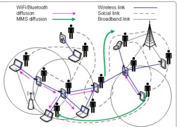
We focus on information diffusion and its optimal control in generalized networks, where the substrate is a wireless multihop network, i.e., user devices. Two different spreading pathways develop in such networks, namely information diffusion via either Multimedia Messaging Service (MMS) in the social layer or via WiFi/bluetooth (P) in the physical substrate [1] (Fig. 1). The former acts as a “long-range” information spread, since nodes communicating directly at the social layer may be actually separated by many hops in the physical layer. MMS transfers act as diffusion shortcuts. On the con-trary, P-type information transfers act as local information ripples over short-range areas around information processors.

(6)

simplicity, mobility is ignored, since compared to an MMS type of information spread-ing, the corresponding long-range information spreading achieved by mobility, which is essentially of P type, will lead to a similar, but smaller effect, as also argued in [1].

We assume M classes of information denoted by m=1...M, as in [24]. Each class con-sists of messages on a specific topic, e.g., summer vacations advertisements. Informa-tion diffusion is studied separately for each class; however, interacInforma-tions among separate classes are taken into consideration in the information diffusion model’s probabilistic setting. Each node i is characterized by its interest in class m at time t, denoted as Rm_i (t) ,

where

∀mRim(t)≤1, ∀i (e.g., normalization over all classes). The information diffu-sion process proposed in this paper is based on the Susceptible–Infected–Susceptible (SIS) epidemic model [9]. We consider the following mapping. A node i is considered Infected (i.e., informed) for a specific class m of information if it possesses at least one message belonging in this class, otherwise i is considered Susceptible (i.e., not informed) for class m. This means that an informed/not-informed node is mapped to an infected/ susceptible state correspondingly, in epidemiology terms. More precisely, the transition from the susceptible state to the infected state for a particular class takes place when a node receives information about this class, while an infected node transits back to the susceptible state when it deletes all messages for this class.

In the rest of the paper, we will employ the notation provided in Table 1. If the network is directed, the out-degree is considered. f1(x),f2(x),f3(x) are general functions that will

be used in the information diffusion model. Finally, the system model will be further enhanced in "Optimal control framework for information diffusion", where the optimal

(7)

control framework over the information dissemination modeling framework in general-ized networks is introduced.

Information diffusion modeling and analysis without control

In this section, we describe the proposed information diffusion process that considers users’ social features/interests. Its analysis via epidemic modeling leads to the incorpo-ration of the impact of nodes’ interests on the information diffusion dynamics. With respect to information diffusion, a node i is expected to perform/experience one of the following actions at each time t.

1. For the classes for which i is infected/informed:

(a) i diffuses information about class m with probability f1(Rmi (t)) (also denoted as f1(t) for simplicity),

(b) i deletes all messages about class m with probability qf2(Rmi (t)), where the

parameter q is introduced to control the deletion process and f2(Rm_i (t)) will be also denoted as f2(t) for simplicity.

We consider that the duration of each time slot permits only the completion of one action, thus only one class m will be selected and either (a) or (b) will hap-pen. This means that

2. Node i performs another action—which is not of interest for the information diffu-sion—with probability equal to 1−

m:i∈Im₍_t₎(f1(Rim(t))+qf2(Rim(t))).

If choosing one class m for action (a) (with probability f1(Rim(t))), node i performs one of the following:

m:i∈Im(t)

(f1(Rmi (t))+qf2(Rmi (t)))≤1.

Table 1 Notation and explanation of symbols.

Symbol Interpretation

Im_(t) _{Number of Infected nodes for class}_m

Sm_(t) _{Number of Susceptible nodes concerning class}_m Im₍_t₎ _{Set of Infected nodes concerning class}_m NS(i) Set of node i’s friends in the social layer

NP(i) Set of connections of i in the wireless network (physical layer)

0≤p1,p2,q≤1 Probabilities defined in the proposed information diffusion model

N_Savg The average degree of all nodes in the social layer

f1(x) f1(x): [0, 1] → [0, 1] monotonically increasing on x f2(x) f2(x): [0, 1] → [0, 1] monotonically decreasing on x

(8)

• with probability p1, node i employs an MMS type of transmission, including as receivers each j∈N_S₍_i₎_{selected with probability}_f₃₍_Rm

j (t)) (also denoted as f3(t) for simplicity), where f3(Rm_j (t)) for all j∈NS(i) does not form a probability distribution,

• with probability p2, node i broadcasts to all its NP(i) neighbors (P-type action).

Note that p1+p2≤1.

The above diffusion process requires that there is always an infected node for every class to maintain the spreading. However, all infected nodes for a particular class may delete their information for this class, thus disrupting its diffusion. Exogenous impact such as the optimal control which will be introduced in "Optimal control framework for information diffusion", may be leveraged to alleviate in a certain degree such phenom-ena of extinction of a whole information class. In the case of P-type contacts, we do not consider the interests of users receiving a P-induced message, as the latter is broadcasted indiscriminately to all of them.

In the following, we model the dynamics of the evolution of the number of infected nodes for each class m, Im(t), via differential equations that approximate the system

evolution. Specifically, the approximate dynamics of Im(t) are captured by the following

ordinary differential equation (ODE),

where f₃avg(t) is the average or the expected value of all f3 functions over the network at time t for the corresponding class m. Functions f₁avg(t), f₂avg(t) are similarly defined. The

initial conditions are Im₍₀₎₌_Im

0 ,∀m, i.e., I0m nodes are initially infected for each infor-mation class m via the social layer.

The ODE (1) has a unique solution when f₁avg(t), f₂avg(t), f₃avg(t) are continuous

functions with respect to time (Cauchy–Lipschitz Theorem [25]). The right-hand side is obviously Lipschitz continuous with respect to Im_{. This fact has an impact on the}

design of possible forms for the interests’ functions Rm_i (t), ∀m,i, which should be

con-tinuous in time. It also has impact on the design of possible formats for the functions f₁avg(t), f₂avg(t), f₃avg(t).

A suitable selection for the functions f1,f2,f3 in the working example scenarios that

follow is:

This configuration is not restrictive in the sense that others may be designed for other scenarios/applications. It is important to note that Eq. (1) is approximate since averages (1)

dIm₍_t₎ dt =p1f

avg 1 (t)f

avg 3 (t)

Sm₍_t₎

N I

m₍_t₎_Navg s

+p2N πR2

L2

Sm(t)

N I

m₍_t₎_favg 1 (t)

−qIm(t)f₂avg(t),

(2)

f1(Rm_i (t))= R

m i (t)

2M ,

f2(Rm_i (t))= 1−R

m i (t)

2M ,

(9)

or expected values of the functions f1,f2,f3 are used. However, such an approximate

form can be used to demonstrate the important characteristics of information diffusion dynamics in specific interesting cases that will be examined via appropriately designed scenarios in the sequel.

Scenario 1: periodic users’ interests

In this scenario, two classes of information are considered. The time continu-ous interests’ functions take sinusoidal forms to express users’ time periodic-ity of their interest with respect to the propagated information. Specifically, R1_i(t)=1−Aisin2(a(t+bi))+Bi, ∀i, for class m=1, where a>0 determines the period of users’ interests and Ai, bi, Bi are appropriately defined constants. Then,

R2_i(t)=Aisin2(a(t+bi))−Bi, ∀i, so that R1i(t)+Ri2(t)=1,∀t,i. Note that, we consider the same frequency for all sinusoidal interests assuming the propagation of information that intrigues the attention of all users over specific time periods such as vacations, summer sports, Halloween, etc.

Based on the configuration for the functions f1,f2,f3 defined above (Eq. 2), their

aver-age values for class 1 become

where bi=b, ∀i, and the constants A, B are computed by averaging the interests over all users at time t. The average values of functions f1,f2,f3 for class 2 are defined similarly.

We can also assume that f₁avg(t), f₂avg(t), f₃avg(t) represent the expected values of the

corresponding functions of users’ interests at time t. Thus, users’ interests will vary ran-domly according to a distribution with mean value 1−Asin2(a(t+b))+B for class 1, letting the complementary interest (i.e., with mean value Asin2(a(t+b))−B) to be

assigned to class 2.

In this case, the ODE (1) for class 1, becomes

and similarly, the ODE (1) for class 2, can be written as f₁avg(t)=1−Asin

2₍_a₍_t₊_b₎₎₊_B

2M ,

f₂avg(t)=Asin

2₍_a₍_t₊_b₎₎₋_B

2M ,

f₃avg(t)=1−Asin2(a(t+b))+B,

(3) dI1₍_t₎

dt =

p1Nsavg N (N−I

1₍_t₎₎_I1₍_t₎(1−Asin2(a(t+b))+B)2 2M

+p2

πR2 L2 (N−I

1₍_t₎₎_I1₍_t₎(1−Asin2(a(t+b))+B) 2M

−qI1(t)(Asin

2₍_a₍_t₊_b₎₎₋_B₎

2M ,

(4) dI2₍_t₎

dt =

p1Nsavg N (N−I

2₍_t₎₎_I2₍_t₎(Asin2(a(t+b))−B)2

2M

+p2 πR2

L2 (N−I

2₍_t₎₎_I2₍_t₎(Asin2(a(t+b))−B)

2M

−qI2(t)(1−Asin

2₍_a₍_t₊_b₎₎₊_B₎

(10)

The solution of both Eqs. (3), (4) takes a complex form which does not provide any intui-tion regarding the dynamics of change of the number of infected nodes for each class,

I1(t), I2(t). For this reason, we apply a finite difference approach to approximate them

as follows. Let M1(t) be the right-hand side of Eq. (3) and M2(t) be the right-hand side of Eq. (4). Then, the finite difference scheme with sufficiently small time step �t>0 and t≥0 yields:

It can be observed that when 1−Asin2(a(t+b))+B∼=0, M1(t)∼= −qI 1₍_t₎ 2M , thus

I1(t+�t) <I1(t) for that time periods, while complementarily S1(t+�t) >S1(t). The converse holds for the time periods where 1−Asin2(a(t+b))+B∼=1. Therefore, the periodicity of user interests is reflected in the information diffusion dynamics, where it is possible that the number of infected nodes does not converge to a specific value but rather fluctuates according to a time period determined by user interest periodicity.

Scenario 2: comparison of information diffusion dynamics among groups with different characteristics

In this scenario, we apply constant interests to study how information of a specific sub-ject spreads in groups characterized by different features such as in the second example described in the introductory section ("Background"). This special case is similar to the SIS models developed in literature [8, 9] in the sense that the parameters applied in the ODEs describing the dynamics of information diffusion are constant, contrary to the time varying parameters (f₁avg(t), f₂avg(t), f₃avg(t)) considered in this paper. Therefore, the

already existing schemes [26] constitute special cases of our proposed diffusion model. In this framework, we consider two groups and one information class (e.g., class 1). For both groups R1_i(t)=a, ∀i, 0<a<1, where for the first group a is close to 1 while in the second group a gets closer to 0. In this particular case of constant interests, the solu-tion of Eq. (1) attains a less complex form than in Scenario 1. However, we will use again the finite difference approximation of Eqs. (5), (6), where the definitions of M1(t), M2(t) are based on constant interests adapted for the two groups correspondingly, to get more intuition about the derived convergence in the number of infected nodes. Specifically, as it will be verified via simulation and numerical results in "Simulation and numeri-cal results without applying control", a higher constant interest by users implies conver-gence of the number of infected nodes to a higher value.

Scenario 3: increasing vs. decreasing users’ interest

In this scenario, there exist two classes of information, while the population has increas-ing interest for the one class and decreasincreas-ing for the other. The appropriate interest func-tions for this case are formulated, ∀i, as follows:

where A, B, C are constants.

(5)

I1(t+�t)=I1(t)+M1(t)·�t,

(6)

I2(t+�t)=I2(t)+M2(t)·�t.

(7)

R1_i(t)=B At At+C, R

2

i(t)=B

(11)

Again, we will use the finite difference approximation of Eqs. (5), (6), where the defini-tions of M1(t), M2(t) for each class correspondingly are based on Eq. (7).

Optimal control framework for information diffusion

In this section, we introduce an optimal control framework for the previously presented information diffusion model for a specific class m. The objective in this optimal control problem is to maximize the number of infected (informed) nodes for a topic/class m by applying an exogenous aid/force, i.e., the control, while taking into account associated control costs, e.g., advertising cost. The motivation behind this is twofold. First it might be necessary to apply a control action to boost users’ interest to increase information spreading. Secondly, more resources might be required (by increasing a control signal) when users are more interested in a topic to conserve resources by not wasting them when users are not interested in the propagated information. Thus, this approach will allow affecting the information diffusion over the susceptible (non-informed) users, via properly controlling user interests.

Assuming the control signal is given by a function u(.)= {u(t)|t∈ [0,T]}, we aim at maximizing the objective function:

where k1,kI ≥0, k2≤0 are parameters expressing the trade-off between control cost and diffusion efficiency. Parameters k1,k2 refer to the operation during a specific time interval within [0, T] and kI refers to the final state of the system. We aim at finding an

optimal control u∗₍_.₎_{such that:}

The control problem will be solved subject to the approximate dynamics of the evolution of the number of informed nodes, which is similar to Eq. (1):

with Im(0)=I₀m (Sm(0)=N−I₀m). Also the following state conditions should hold:

for every t. Note that Eq. (10) differs from Eq. (1) due to the introduction of the con-trol u(t) in the summands of its right-hand side, where the probabilities f₁avg(t), f₂avg(t)

have been replaced with f₁avg(t)g1(u(t)), f2avg(t)g2(u(t)). The control u(.) depends

on the controller’s budget for topic m, while the control region is defined as �= {u(.): [0,T] →R_|u_min≤u(t)≤umax, ∀t} and also each u(.) is a piece-wise continuous function such that its left and right limits exist. Functions g1,g2 are non-negative, differentiable and either convex or concave with respect to u. While g1 is

(8) J(u(.))=

T

0

k1Im(t)+k2u(t)

dt+kIIm(T),

(9)

J(u∗(.))=max

u(.) J(u(.)).

(10) dIm(t)

dt = Nsavgp1

N f

avg 1 (t)f

avg

3 (t)(N−Im(t))Im(t)g1(u(t))

+p2 πR2

L2 f avg

1 (t)Im(t)(N−Im(t))g1(u(t))

−qIm(t)f₂avg(t)g2(u(t)),

(12)

increasing with u, g2 is decreasing, and g1,g2: [umin,umax] → [0, 1]. The control might take the form of incentives for increasing user interest, or it may exploit the increased user interest to reinforce information spreading, while such behavior will be explored in the following.

The next proposition allows us to ignore the state constraints expressed in Eq. (11) in the rest of the analysis.

Proposition 1 For any u(.)∈�, the state function Im₍_.₎_{: [}_0,_T_{] →}_R _{that satisfies}

Im(0)=I₀m, also satisfies Eq. (11).

Proof Let t0 be the first time instant in [0, T] where Im(t0)=0 or Im(t0)=N.

• If Im(t0)=0 then Sm(t0)=N and dI

m₍_t₎

dt |t=t₀+ =0, meaning that Im(t)=0, for every t>t0, t≤T.

• If Im(t0)=N then Sm(t0)=0. Thus, dI

m_(t)

dt |t=t₀+= −qN f avg

2 (t0)g2(u(t0)) <0, since f₂avg(t0),g2(u(t0)) >0, meaning that Im(t0+)≤N. Similarly for all other t′∈(t0,T]

where Im(t′)=N.

The following proposition proves that the number of infected nodes for class m, Im(t)

is strictly positive for every t∈ [0,T].

Proposition 2 We have thatIm(t)≥I₀me−qf

avg

2maxg2(umin)t≥0, ∀t∈ [0,T].

Proof It holds that dIm_(t)

dt ≥ −qIm(t)f avg

2 (t)g2(u(t)), which means that Im_(t)′

Im_(t) ≥ −qf

avg

2maxg2(umin), where f2 maxavg =max∀tf avg

2 (t) and since g2 is decreasing with

u. Thus, lnIm₍_t₎_{≥ −qf}avg

2maxg2(umin)t+lnI

m₍₀₎_{, yielding}_Im₍_t₎_≥_Im 0e

−qf_2maxavg g2(umin)t, for

every t∈ [0,T].

Definition 1 The pair (Im(.),u(.)) is an admissible pair if the following hold: (i)

u(.)∈� , (ii) the state (Im(.)) constraint of Eq. (10) holds. Then u(.) is called an

admis-sible control [20].

Definition 2 An admissible control u(.) is an optimal control, if J(u(.))≥J(u(.)) for all

admissible controls u(.) [20].

Based on these two definitions, we will apply Pontryagin’s Maximum Principle [20, 27–29] to determine the optimal control’s functional form and study its properties. Let us denote as (t) the adjoint/costate variable of the Pontryagin’s Maximum Principle [27]

at time t∈ [0,T]. First, we define the Hamiltonian function, H, at time t as:

(12)

H₍_Im₍_t₎_,_u₍_t₎_,₍_t₎₎₌_k

1Im(t)+k2u(t)

+₍_t₎

Nsavgp1

N f

avg 1 (t)f

avg

3 (t)(N−Im(t))Im(t)g1(u(t))

+p2 πR2

L2 f avg

1 (t)Im(t)(N−Im(t))g1(u(t))

− qIm(t)f₂avg(t)g2(u(t))

(13)

Assuming that u∗₍_.₎_{is the optimal control value and}_Im∗

(.) is the corresponding state

tra-jectory, i.e., the one solving Eq. (10) for u∗₍_.₎_{, according to Pontryagin’s Maximum} Prin-ciple [27], there exists a function ∗(.): [0,T] →R such that

where ∗₍_.₎_{is the optimal costate (adjoint) function and also the optimal control,}_u∗₍_.₎_{, is} computed as:

For simplicity, from now on we omit the symbol ∗_{from the optimal values. We can prove} the following proposition which will be useful in studying the properties of the optimal control function.

Proposition 3 We have that(t) >0for t∈ [0,T).

Proof We follow a similar proof to the one of Lemma 2 in [20]. First we show that (t)

is strictly positive over an interval of non-zero length towards the end of [0, T). It holds that ₍_T₎₌_k_I _≥₀. If _k_I _>₀, this statement holds due to continuity. If _k_I=0, then from (13) and for t=T we have: d_dt(t)|t=T = −k1<0, i.e., descending from positive values before reaching the value kI =0, and this statement also holds.

As t′<T, consider the latest time in [0, T) that (t′)=0, i.e., (t) >0 for t′<t<T . Then, d(t)

dt |t=t′+ = −k₁<0 which is impossible since for t>t′, is positive and thus it should increase from the zero value. The latter statement concludes the proof of

Propo-sition 3.

Let us now omit the time dependence over the employed notation for brevity reasons. We can define the functional:

(13)

d∗(t) dt = −

∂H

∂Im = −k1− ∗₍_t₎

Nsavgp1

N f

avg 1 (t)f

avg

3 (t)(N−2Im∗(t))g1(u∗(t))

+p2 πR2

L2 f avg

1 (t)(N−2Im

∗

(t))g1(u∗(t))

− qf₂avg(t)g2(u∗(t))

,

(14)

∗₍_T₎₌_k_I₍_{transversality condition}₎_,

(15) u∗(t)=u(t)∈arg max

u∈�

H_(Im∗_(t),_u,∗_{(t)), 0}≤t≤T.

(16)

φ (u)=k2u+

Nsavgp1

N f

avg 1 f

avg

3 (N−Im)Img1(u)

+p2 πR2

L2 f avg

1 Im(N−Im)g1(u)

− qImf₂avgg2(u)

(14)

and search for an optimal u, i.e., such that φ (u)≥φ (u) for all admissible u∈. The functional φ (u) is derived by the Hamiltonian (Eq. 12) for a particular time, considering only the terms that depend on u.

Given the possible forms of the functions g1,g2 with respect to the control u (convex or concave), the following cases can be identified:

1. g1 convex and g2 concave. Then φ is convex with respect to u. Due to convex maxi-mization, the optimal control will be necessarily at the extrema of the range of the control, determined by comparison as:

2. g1 concave and g2 convex. Then φ is concave with respect to u. In this case, a concave maximization takes place, where the maxima of φ (u) occur at the points where the

partial derivative with respect to u is zero, or at the extrema of the range of the con-trol, determined by comparison. The equation ∂φ

∂u =0 becomes:

where _>₀ from Proposition 3. If _u′_{is the solution of the above, then the optimal}

control becomes:

In this case based on the explicit forms of functions g1, g2, we can study possible rela-tions/properties of the optimal control with respect to users’ interests, as it will be performed in the following sections.

3. g1 concave and g2 concave. We have

where A1= Nsavgp1

N f

avg 1 f

avg

3 (N−Im)Im ∂2_g1_(u)

∂u2 +p2πR 2 L2 f

avg

1 Im(N−Im) ∂2_g1_(u)

∂u2 ≤0

and B1=qImf2avg ∂2g2(u)

∂u2 ≤0. Thus, ∂2φ (u)

∂u2 ≤0 if |A1| ≥ |B1|, that leads to a concave maximization as in case 2 above, or ∂2φ (u)

∂u2 ≥0 if |A1| ≤ |B1|, that leads to a convex maximization as in case 1 above.

4. g1 convex and g2 convex. Then ∂

2_g1_(u) ∂u2 ≥0,

∂2g2(u)

∂u2 ≥0. Thus, ∂2_{φ (u)}

∂u2 ≥0 if |A1| ≥ |B1| , that leads to a convex maximization as in case 1 above, or ∂2_{φ (u)}

∂u2 ≤0 if |A1| ≤ |B1|, that leads to a concave maximization as in case 2 above.

(17)

u∗=

umin ifφ (umin) > φ (umax),

umax ifφ (umin) < φ (umax).

(18)

−k2

=

∂g1(u)

∂u

Nsavgp1 N f

avg 1 f

avg

3 (N−Im)Im

+p2

πR2

L2 f avg

1 Im(N−Im)

− ∂g2(u)

∂u qI

m_favg 2 ,

(19)

u∗=max

umin, min{u′,umax}

.

(20)

∂2φ (u) ∂u2 =

Nsavgp1

N f

avg 1 f

avg

3 (N−Im)Im ∂2g1(u)

∂u2

+p2 πR2

L2 f

avg

1 Im(N−Im) ∂2g1(u)

∂u2

−qImf₂avg∂

2_g 2(u) ∂u2

(15)

We should note that the controller applies one kind of control with aim to increase Im(t) trading-off cost, but this impacts in a different way each part of the information

propagation equation (i.e., Eq. 10) via the functions g1(u),g2(u).

At this point, we study the case 2 more extensively, by choosing a (non-restrictive) specific form for the control functions g1(u), g2(u), as follows:

This choice serves the purpose of boosting the number of infected (informed) nodes for the examined class by increasing probabilities of communicating/transferring knowledge via g1(u) >1 in the first and second summands of the right-hand side of Eq. (10), and by decreasing probabilities of knowledge “deletion” via g2(u) <1 in the last summand of the right-hand side of Eq. (10). Then, after computing ∂g1(u)

∂u , ∂g2(u)

∂u , replacing them in Eq. (18) and solving the latter, the optimal control takes the following formula:

where { }umax

umin expresses projection to [umin,umax] and

At this point, we study some properties of Ŵ (Eq. 23) that will assist in the interpreta-tion of the observable behavior of the optimal control in "Simulainterpreta-tion results, numerical results and discussion in controlled information diffusion". First, we study the depend-ence of Ŵ on the values of interest for the examined class m, i.e., Rm_avg. By considering Eq.

(2) providing the types of f₁avg, f₂avg, f₃avg, Ŵ is increasing with Rm_avg, i.e., _∂∂Ŵ_Rm

avg >0 if

Therefore, Ŵ will become an increasing function of interest for class m only if the num-ber of infected nodes for class m becomes less that the threshold ITH. This behavior is also expected for the optimal control itself, u∗ (Eq. 22), since by Proposition 3 it holds −_k

2 >0 (if ignoring the dependence of on R

m

avg). This fact, which will be verified via

numerical evaluations in "Simulation results, numerical results and discussion in con-trolled information diffusion", indicates the targeted trade-off between information spread and cost, while leveraging users’ interests for class m. If the number of infected nodes for class m is high enough, higher that ITH, the optimal control saves resources when the corresponding user interest for class m increases. When the number of

(21) g1(u)=1+

ln(1+u) ln(1+umax)

,

g2(u)=

ln(1+umax)−ln(1+u))

ln(1+umax)

.

(22) u∗=

−1−Ŵ

k2

umax

umin ,

(23)

Ŵ = 1

ln(1+umax)

Nsavgp1

N f

avg

1 f

avg

3 (N−Im)Im+p2

πR2 L2 f

avg

1 Im(N−Im)

+qImf₂avg

.

(24)

Im<N− q Nsavgp12Rmavg

N +

p2πR2 L2

(16)

infected nodes falls below ITH, the control increases with user interest, aiming to lever-age from higher values of interest to drastically boost the number of infected nodes for class m. This behavior emerges also in the case of power control in a wireless channel, where high power values are optimal under good channel conditions, to exploit the max-imum possible data transfer rates [30]. Since ITH (Eq. 24) is time varying, as Ravgm evolves

with time ("Information diffusion modeling and analysis without control"), the monot-ony of Ŵ may also change with time. Generally, higher values of R_avgm lead to a higher

range of values of the number of infected nodes for which Ŵ is increasing with interest for class m.

Obviously, Ŵ is a concave function of Im_{, attaining its maximum at}

I_maxm =

FRm

avg+G(Rm_avg1 −1)+K DRm

avg+E , where F=

NSavgp1

2M , E =

p2πR2 L2_M, D=

NSavgp1

MN , G=

q 2M,

K= p2πR2N

L2₂_M . Note that Imaxm is decreasing with interest when

(FE+GD−DK)(Rm

avg)2−2GDRavgm −GE<0, where D, E, F, G, K, are determined by the parameters of the system. In this case, for higher values of interest it is intuitively expected that the optimal control (Eq. 22) will achieve its maximum on a lower value of Im, if ignoring any dependence of on the examined parameters, i.e., _Im_,_Rm_avg.

Computing the optimal control value

Although Eqs. (17, 19) provide the form of the optimal control, computing the optimal control value is more complex, demanding the knowledge of the value of the adjoint variable, , for each t. In this section, we construct the Hamilton–Jacobi–Bellman (HJB) equation [27–29] and solve it via a numerical approach to obtain optimal control values within the control time interval ([0, T]).

Definition 3 We define the Value function V(Im,t), where Im(t)=Im∈R, 0≤t≤T , as follows:

Actually, the Value function is obtained by varying the starting time of control within the control interval [0, T] and the initial value of infected nodes for class m. The HJB equation is formulated as the following partial differential equation:

where H_{is the Hamiltonian function defined in Eq. (12). Also, at each time}_t_{∈ [0,}_T], we have ∂V(Im∗_(t),t)

∂Im =∗(t), where the symbol ∗ again is used for denoting the optimal values obtained for u∗₍_t₎_{. At this point, we will solve numerically the HJB equation [31] (Eq. 25)} to compute the Value function for each t∈ [0,T). Then, the optimal control values will be obtained via Eqs. (17, 19) if replacing with ∂V

∂Im both computed at the examined time t. Applying a finite difference scheme and denoting as u(t) the optimal control value, Eq. (25) takes the following form:

V(Im,t)= sup u(.)∈�

J(u(.)), V(Im,T)=kIIm(final condition).

(25)

dV(Im,t)

dt +maxu∈� H

Im,u,∂V(I m_,_t₎

∂Im

=0,

(17)

where Im, t are the steps of state and time and Eq. (26) is solved backwards since we know the Value function at the end, T, of the control time interval. Specifically, we com-pute the Value function for all Im∈ {1, 2, ...,N} at time 0≤t−�t<T from the corre-sponding ones at time t. When computing the optimal control values via Eqs. (19), (17) we replace with ∂V

∂Im

t=

V(Im₊_�_Im_,_t₎₋_V₍_Im₋_�_Im_,_t₎

2�Im . Furthermore, in the numerical solu-tion of the HJB, we apply as a boundary condisolu-tion for the partial derivative of the Value function with respect to state the following ∂V

∂Im

t=T = ∂V ∂Im

t=T−�t.

Simulation and numerical results without applying control

In this section, we present simulation and numerical results for each users’ interest sce-nario of "Information diffusion modeling and analysis without control". Specifically, the simulation results refer to the realization of the diffusion model described in "Informa-tion diffusion modeling and analysis without control" in MATLAB, while numerical results refer to the approximate solution (via finite difference scheme) of the ODEs in each scenario with the same parameters as in the corresponding simulation.

The simulation setting is as follows. We consider a generalized network, the wire-less substrate of which consists of a wirewire-less multihop network with N =500 nodes deployed over a square region with side L=350m and with homogeneous transmis-sion radius among nodes equal to R=25m. All simulation results are obtained as

aver-ages over several wireless topologies (#2) and multiple repetitions (#3) for the diffusion

at each topology. Furthermore, we examine two overlaying social network topologies over the same set of nodes as the wireless substrate, namely one scale-free and one small-world [32]. For the scale-free network topology, the social degree for each node is drawn from the power-law distribution with exponent 3, as observed for many social networks [33] (specifically the probability density function is f(x)=

2 x

3

, x≥2), and the corresponding social layer’s neighbors of each node are chosen randomly. The small-world topology is constructed following the Watts & Strogatz paradigm [34]. For both topologies, N_Savg∼=4. However, the degree distribution in the small-world topol-ogy is much more homogeneous than the corresponding one of the scale-free social topology. Also, the scale-free topology presents low average path length, which is a small-world feature [32]. Note that the value t should be appropriately small, so that the solution of the ODE derived via the finite difference scheme (Eqs. 5, 6), approxi-mates closely the precise solution of the ODE. We chose t=0.4. Finally, 10 nodes out of 500 are initially infected (e.g., via MMS) for each class in all simulation and numeri-cal results that follow.

(26)

V(Im,t)−V(Im,t−�t)

�t +k1I

m₊_k 2u(t)

+ V(I

m₊_�_Im_,_t₎₋_V₍_Im₋_�_Im_,_t₎

2�Im

Nsavgp1

N f

avg 1 (t)f

avg

3 (t)(N−Im)Img1(u(t))

+ p2 πR2

L2 f avg

1 (t)Im(N−Im)g1(u(t))−qImf2avg(t)g2(u(t))

=0,

(18)

Scenario 1: information diffusion dynamics in the case of periodic users’ interests

In this scenario, we consider that the users’ interests vary uniformly and randomly with mean value 1−1₄sin2(₁₈₀π (t+100))− ₇1 for the first class and 1₄sin2(₁₈₀π (t+100))+ 1₇ for the second class with the constraint that the interests of one node for the two classes are complementary (i.e., in the corresponding scenario of "Information diffusion mod-eling and analysis without control", A= 1₄, B= −1₇, a= ₁₈₀π , b=100). Therefore, the period of the interests’ functions is one year, a fact that can be reflected in realistic situ-ations as the ones explained in "Background". The values of p1, p2, q will be specified in each simulation case.

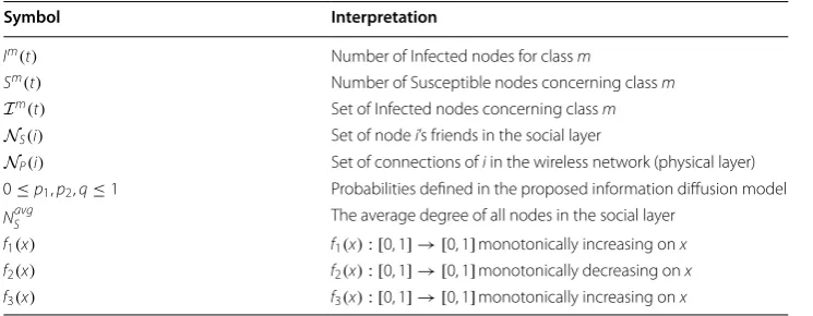
Fig. 2a compares the dynamics of the information diffusion for class 1 as derived by numerically solving Eq. (3) with the results obtained via simulations according to the proposed diffusion model in "Information diffusion modeling and analysis with-out control". The same is illustrated in Fig. 2b for class 2 (where the numerical results are obtained via numerically solving Eq. 4). The involved parameters take the values p1=p2=0.5, i.e., P and MMS types of transfer take place with the same probability in

case of diffusion and q=0.2. The results are the same independently of the social topol-ogy, i.e., small-world or scale-free.

The periodic behavior of users’ interests is also reflected in the dynamics of informa-tion diffusion, as expected from the discussion in "Informainforma-tion diffusion modeling and analysis without control", and the number of infected nodes does not converge to a spe-cific value as predicted by the conventional models in the literature [1, 13]. We observe that for class 1, the numerical results approximate well the ones obtained from simula-tions. In the case of class 2, i.e., in the case of lower interest for the information under propagation, it can be stated that the numerical results mostly overestimate the number of infected nodes. This observation can be explained by the fact that in the simulations, the number of infected nodes may become zero when all nodes delete their messages for a particular class, whereas according to Proposition 2, the theoretical number of infected nodes is always greater than zero. Thus, in the simulation it becomes likely that the information propagation for a class terminates (a fact that becomes more probable when interest values are lower), whereas in theory there is always enough quantity of infected nodes to spread information if the users’ interest for the latter increases.

The results in Fig. 3a, b concern only the case of P type, while the results in Fig. 4a, b refer to the case of applying MMS type alone. By comparing these figures, it is observed

0 50 100 150 200 250 300 350 0

100 200 300 400 500

Time of simulation

Number of Infected Nodes

(class 1)

Simulation, Scale−free Simulation, Small−world Numerical results

a Class 1.

0 50 100 150 200 250 300 350 0

100 200 300 400 500

(class 2)

b Class 2.

Fig. 2 P & MMS types of information diffusion dynamics for periodic interests, with parameters p1=p2=0.5,

(19)

that P type plays a significant role in maintaining the diffusion alive with respect to class 2 in which users’ interest for the diffused information attains lower values. Generally, P type further boosts information spreading for both classes. In Fig. 4a, for class 1, the diffusion dynamics over the small-world topology approximate much closer the numeri-cal results than over the snumeri-cale-free topology, whereas in the other cases, both topologies present similar behavior.

To conclude for this scenario, the theoretical model overestimates the volume of the information spreading, especially for class 2, which is characterized by lower values of interest. Also, the behavior in both cases of social topologies, i.e., small-world and scale-free, does not differentiate significantly.

Scenario 2: information diffusion dynamics in the presence of groups with different characteristics

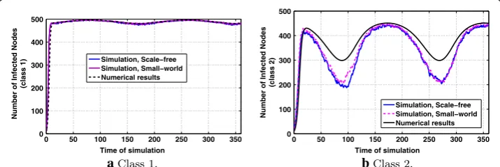
In this evaluation scenario, based on the description of "Information diffusion modeling and analysis without control", we consider one information class and two groups with dif-ferent interests in this information class. Group 1 has an interest value of 0.8 and Group 2 has an interest value of 0.2. Fig. 5a, b indicate that the interest plays significant role in the number of infected nodes to which the dynamics of information diffusion converge. In Group 1 the participants of which are highly interested in this information class, finally all nodes become infected. The parameters’ values are specified in the legends of the figures.

0 50 100 150 200 250 300 350 0

100 200 300 400 500

Number of Infected Node

s

(class 1)

a Class1.

0 50 100 150 200 250 300 350 0

100 200 300 400 500

s

(class 2)

b Class2.

Fig. 3 P type of information diffusion dynamics for periodic interests, with parameters p1=0,p2=1,

q=0.6

0 50 100 150 200 250 300 350 0

100 200 300 400 500

s

(class 1)

a Class 1.

0 100 200 300 400

0 5 10 15 20

s

(class 2)

b Class 2.

Fig. 4 MMS type of information diffusion dynamics for periodic interests, with parameters p1=1,p2=0,

(20)

It is also observed that for high interest the approximation of the theoretical model to the simulation results is satisfactory, while for lower interest, the theoretical model overesti-mates the simulation results. However, in the latter case (Fig. 5b), the diffusion dynamics over the small-world topology obtained via simulations lie much closer to the numerical results. In Fig. 5a, where interest values are higher, both social topologies present similar behavior concerning the information diffusion dynamics.

Scenario 3: information diffusion dynamics in the case of increasing vs. decreasing users’ interests

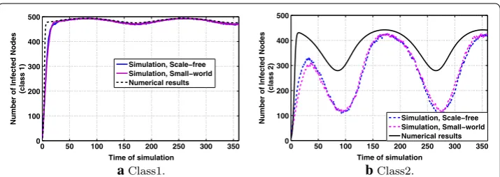
The results regarding this evaluation scenario are shown in Fig. 6a, b, where

A=5,C=10, B=0.5 in Eq. (7). Fig. 6a, demonstrates the dynamics of information diffusion for the first class, where it is observed that the number of infected nodes ini-tially presents a steep increase and then it increases with much lower rate. Regarding the information diffusion dynamics for class 2, from Fig. 6b it is observed that there is an initial increase which later deflates, due to the decreasing with time user interests, even-tually yielding zero number of infected nodes for the simulation results and close to zero number of infected nodes for the numerical results (Proposition 2). Such dynamics can-not be captured by previous state-of-the art information diffusion models using constant diffusion parameters.

0 50 100 150 200 250 300 350 0

100 200 300 400 500

s

(class 1)

a Group 1.

0 50 100 150 200 250 300 350 0

50 100 150 200 250 300 350 400

s

(class 2) _{Simulation, Scale−free}

Simulation, Small−world Numerical results

b Group 2. Fig. 5 P & MMS types of information diffusion dynamics for constant interests, with parameters p1=0.6,p2=0.4, q=0.2

0 50 100 150 200 250 300 350 0

100 200 300 400 500

(class 1) Simulation, Scale−freeSimulation, Small−world Numerical results

a Class 1.

0 100 200 300 400

0 10 20 30 40 50

(class 2)

b Class 2.

(21)

Simulation results, numerical results and discussion in controlled information diffusion

In this section, we further study and evaluate the introduction of control—as described in "Optimal control framework for information diffusion"—in the three scenarios of "Simulation and numerical results without applying control". The values of the parame-ters that are used in "Simulation and numerical results without applying control" remain the same, except otherwise mentioned. Additionally, we consider umin=0,umax =30 ,

Im=1, ∀m, t=10−4_,_k

1=1,k2= −3,kI=1, T =2, and finally, the topology on

the social layer is considered as scale free. Note that �t<< �Im so that the HJB solu-tion converges [31]. The control is applied to only one class (or equivalently one group for constant interests) and specifically, we chose the class m=2 (or equivalently Group 2 for constant interests), to evaluate how information diffusion behaves under low val-ues of interest when introducing control, and compare this behavior with the case when no control is applied (similarly to "Simulation and numerical results without applying control"). In the following subsections, in each scenario, we compare the numerical (derived via Eq. 10 using Eq. 21) and simulation results with and without control regard-ing the number of infected nodes for the second class/group, while we also study several properties and the behavior of the optimal control itself. We adapt the diffusion model of "Information diffusion modeling and analysis without control" to introduce control by replacing the probabilities f₁avg(t), f₂avg(t) with f₁avg(t)g1(u(t)), f2avg(t)g2(u(t)), as

implied by comparing Eq. (10) with Eq. (1). Every simulation runs for 200 time steps, i.e., the control time T =2 is divided into smaller time intervals each having a duration of 0.01.

Scenario 1: controlled information diffusion dynamics in the case of periodic users’ interests

Similar to "Scenario 1: information diffusion dynamics in the case of periodic users’ interests", we consider that the users’ interests vary uniformly and randomly with mean value 1−1₄sin2(_0.5π(t+0.2))− ₇1 for the first class and 1₄sin2(_0.5π(t+0.2))+ 1₇ for the second class with the constraint that the interests of one node for the two classes are complementary.

(22)

absence of control that is also discussed in "Scenario 1: information diffusion dynam-ics in the case of periodic users’ interests". Finally, Fig. 7c zooms in two specific periods of Fig. 7b, after the convergence of the numerical solution of Eq. (10), to indicate in a clearer way the periodicity in the information diffusion dynamics.

0 0.2 0.4 0.6 0.8 1 1.2 1.4 1.6 1.8 2 0

50 100 150 200 250 300 350 400 450 500

Time

without control with control

a

Comparison of simulation results with and without con-trol for 2 time periods.

0 20 40 60 80 100 120 140 160 180 200 0

100 200 300 400 500

Time

b Comparison of numerical results with and without

con-trol for 200 time periods.

40 40.2 40.4 40.6 40.8 41 41.2 41.4 41.6 41.8 42

400 410 420 430 440 450 460 470

Time

s

c Zoom in Fig. 7(b) for 2 time periods after convergence.

(23)

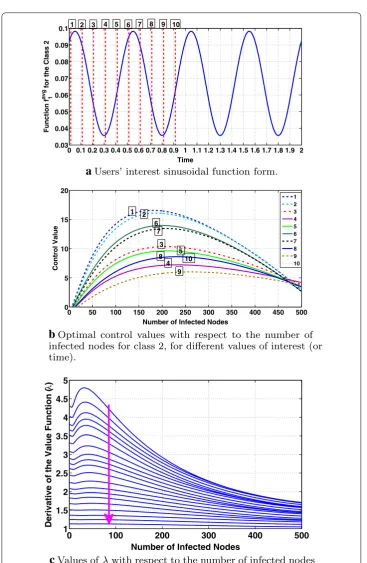
Figure 8 studies the behavior of the optimal control with respect to the number of infected nodes and the users’ evolving interest for the class m=2. From Fig. 8b, we observe that the optimal control is a concave function of the number of infected nodes

0 0.1 0.2 0.3 0.4 0.5 0.6 0.7 0.8 0.9 1 1.1 1.2 1.3 1.4 1.5 1.6 1.7 1.8 1.9 2 0.03

0.04 0.05 0.06 0.07 0.08 0.09 0.1

Time

Function

f1

av

g for the Class

2

1 2 3 4 5 6 7 8 9 10

a

Users’ interest sinusoidal function form.

0 50 100 150 200 250 300 350 400 450 500

0 5 10 15 20

Control Valu

e

1 2 3

4 5 6 7 8 9 10 5

3

4 2 1

6 7

8

9 10

b

Optimal control values with respect to the number of

infected nodes for class 2, for different values of interest (or time).

0 100 200 300 400 500

1 1.5 2 2.5 3 3.5 4 4.5 5

Derivative of the Value Function

(

λ

)

c

Values of λwith respect to the number of infected nodes

for class 2, for different values of interest (or time).

(24)

(for all times), achieving its maximum value at a different number of infected nodes, I_maxm , at each time or value of interest. This behavior is intuitively expected from the analysis of "Optimal control framework for information diffusion" with respect to Ŵ (Eq. (23)), although it ignores the dependence of the adjoint variable on the number of infected nodes. Furthermore, comparing Fig. 8a, b, we observe that I_maxm decreases with interest which can be intuitively explained by the fact that for our considered param-eters the corresponding condition stated at the end of "Optimal control framework for information diffusion" is satisfied. More specifically, higher values of interest, e.g., points 1, 2, 6, 7 of the users’ interest sinusoidal function in Fig. 8a lead to lower values of I_maxm as it is observed in the corresponding optimal control curves 1, 2, 6, 7 in Fig. 8b. More-over, comparing Fig. 8a, b and more specifically the interest values 1, 2, ..., 10 in Fig. 8a with their corresponding control curves in Fig. 8b, it can be observed that the values of the optimal control follow a sinusoidal-like evolution being aligned with the sinusoidal evolution of users’ interest. The decreasing with time trend in the optimal control values, which cannot be explained by the Ŵ function (Eq. 23, "Optimal control framework for information diffusion"), can be justified by the decreasing values of the adjoint variable with time as shown in Fig. 8c where time is indicated by the arrow.

Finally, Fig. 9 shows the monotonicity of the optimal control with respect to interest for different values of the number of infected nodes for class m=2. The applied param-eters in these simulations lead to a threshold value ITH ("Optimal control framework for information diffusion") at most (considering the maximum value of users’ interest) equal to 473 nodes. Thus, it is expected that when Im=2_>₄₇₃_{nodes the optimal control} will be decreasing with interest and the opposite will hold for Im=2_<₄₇₃_{nodes. This} expectation is verified in Fig. 9, where the monotonicity change is performed around Im=2=470 nodes, while below 470 the optimal control value increases with interest (Fig. 9a–e) and above this value (Fig. 9g, h) it decreases with interest balancing in this way the cost with the information propagation efficiency as also discussed in "Optimal control framework for information diffusion". Note that in Fig. 9, the ticks on the hori-zontal axis are not simple interest values, but they are the values of interest over a two-period time interval as shown in Fig. 8a. Therefore, time has also impact on the adjoint variable affecting the optimal control values leading, e.g., here to decreasing optimal control values with time as it can be observed in all subfigures of Fig. 9. Time evolution is denoted by the arrows in each subfigure of Fig. 9.

Scenario 2: controlled information diffusion dynamics in the presence of groups with different characteristics

(25)

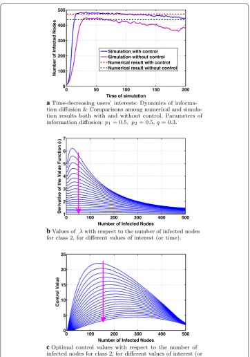
the case of periodic users’ interests"). As it is shown in Fig. 10a, introducing control leads to a tighter approximation of the simulation results from the numerical ones, compared to the absence of control.

Figure 10c studies the behavior of the optimal control with respect to the number of infected nodes and time for the class m=2. As in Fig. 8b, we observe that the optimal control is a concave function of the number of infected nodes (for all times) while Im

max

0.030 0.04 0.05 0.06 0.07 0.08 0.09 0.1 2

4 6 8 10

Values of f₁avg_Function

Values of Control

Number of Infected Nodes=50

a

0.030 0.04 0.05 0.06 0.07 0.08 0.09 0.1 5

10 15 20

b

0.030 0.04 0.05 0.06 0.07 0.08 0.09 0.1 5

10 15 20

Values of f₁avg Function

c

0.032 0.04 0.05 0.06 0.07 0.08 0.09 0.1 4 6 8 10 12 14

d

0.032 0.04 0.05 0.06 0.07 0.08 0.09 0.1 3

4 5 6 7

Values of Contro

l

e

0.032 0.04 0.05 0.06 0.07 0.08 0.09 0.1 2.5 3 3.5 4 4.5 5

l

f

0.032 0.04 0.05 0.06 0.07 0.08 0.09 0.1 2.5 3 3.5 4 4.5 5

l

g

0.03 0.04 0.05 0.06 0.07 0.08 0.09 0.1 1.5 2 2.5 3 3.5 4 4.5

l

h

(26)

remains approximately stable (due to the consideration of constant interests). The opti-mal control values decrease with time (indicated by the arrow) due to the decreasing values of the adjoint variable with time as shown in Fig. 10b.

0 50 100 150 200

0 100 200 300 400 500

Simulation with control Simulation without control Numerical result with control Numerical result without control

a Time-constant users’ interests: Dynamics of information diffusion & Comparisons among numerical and simulation results both with and without control. Parameters of infor-mation diffusion:p1= 0.5, p2= 0.5,q= 0.3.

0 100 200 300 400 500

1 1.5 2 2.5 3 3.5 4

Derivative of the Value Function

(λ

)

b Values ofλwith respect to the number of infected nodes for Group 2, for different values of time (interest is constant with time).

0 100 200 300 400 500

0 2 4 6 8 10 12

c Optimal control values with respect to the number of infected nodes for Group 2, for different values of time (in-terest is constant with time).