Optical soliton perturbation of Fokas-Lenells equation by the Laplace-Adomian decomposition algorithm

(1)

R E S E A R C H

Open Access

Optical soliton perturbation of

Fokas-Lenells equation by the

Laplace-Adomian decomposition algorithm

O. González-Gaxiola

1*

, Anjan Biswas

2,3,4

and Milivoj R. Belic

5

Abstract

This paper displays numerical simulation for bright and dark optical solitons that emerge from Fokas-Lenells equation which is studied in the context of dispersive solitons in polarization-preserving fibers. The Laplace-Adomian

decomposition scheme is the numerical tool adopted in the paper. The numerical results, for bright and dark solitons, are expository and therefore supplement the analytical developments, thus far.

Keywords: Fokas-lenells equation, Polarization-preserving fibers, Adomian decomposition method, Optical solitons solutions, Perturbation

Introduction

One of the governing models to study dispersive soli-tons is Fokas-Lennels equation (FLE) [1–13]. In such a model, in addition to group velocity dispersion (GVD), one considers, inter-modal dispersion as well as nonlin-ear dispersion thus treating it with a flavor of additional dispersive effects. There has been a plethora of analyti-cal tools that have been implemented to study FLE. They range from semi-inverse variational principle, Lie sym-metry analysis, Riccati equation approach, exp-function method, traveling wave hypothesis, trial function method and further wide varieties. This paper will be changing gears to study the model from a different perspective. One of the very many and modern numerical algorithms that will be implemented is the Laplace-Adomian decomposi-tion integradecomposi-tion scheme. This method has been success-fully applied to variety of other models from optics [14–

16]. This paper now studies FLE, for the first time, by the aid of Laplace-Adomian decomposition scheme. The details are sketched in the remainder of the paper, after introducing the model.

*Correspondence:ogonzalez@correo.cua.uam.mx

1_{Departamento de Matemáticas Aplicadas y Sistemas, Universidad Autónoma} Metropolitana-Cuajimalpa, Vasco de Quiroga 4871, 05348, Mexico City, Mexico Full list of author information is available at the end of the article

The Fokas-Lenells equation (FLE) in presence of perturbation terms

The dimensionless form of the perturbed Fokas-Lenells equation (FLE) is given by

iut+a1uxx+a2uxt+ |u|2(bu+iσux)

=iαux+λ

|u|2u_x +μ|u|2_xu. (1) This equation was first studied in [17–24] and arises in various systems such as water waves, plasma physics, solid state physics and nonlinear optics. In Eq. (1),u(x,t) repre-sents a complex field envelope, andxandtare spatial and temporal variables, respectively. Here, the coefficienta1is

the group velocity dispersion (GVD) anda2is the

spatio-temporal dispersion (STD) the coefficientbis self-phase modulation moreover σ accounts for nonlinear disper-sion. In the perturbative term of Eq. (1), the first term represents the inter-modal dispersion (IMD), the sec-ond term is the self-steepening effect and finally the last term accounts for another version of nonlinear dispersion (ND).

Bright optical solitons

The bright optical soliton solution to (1) is given by [5,11]:

u(x,t)=Asech [(x−νt)]ei[−κx+ωt+θ]. (2) Here,νis the soliton velocity,κis the soliton frequency,ω is the angular velocity andθ is the phase center.

(2)

The amplitudeAof the soliton in this case is given by

A= ±

2(a1−a2ν)

b−κλ+κσ, (3)

where, the velocity of the soliton in relation to the coeffi-cients that appear in the Eq. (1) is

ν= α+2a1κ−a2ω a2κ−1

, (4)

and the constraints conditions on the parameters are

a2κ=1, 3λ+2μ−σ=0. (5)

In the previous contextκ is any parameter that satisfies the Eq. (5).

Dark optical solitons

noindent The dark optical soliton solution to (1) is given by [5,11]:

u(x,t)=Btanh [(x−νt)]ei[−κx+ωt+θ]. (6) Here,νis the soliton velocity,κis the soliton frequency,ω is the angular velocity andθis the phase center.

The amplitudeBof the soliton in this case is given by

B= ±

−2(a1−a2ν)

b−κλ+κσ , (7)

where, the velocity of the soliton in relation to the coeffi-cients that appear in the Eq. (1) is

ν= α+2a1κ−a2ω a2κ−1

, (8)

and the constraints conditions on the parameters are

a2κ=1, 3λ+2μ−σ=0. (9)

In the previous contextκ is any parameter that satisfies the Eq. (9).

The Laplace Adomian Decomposition Method (LADM)

To illustrate the basic concept of Laplace-Adomian decomposition algorithm, we consider the general form of second order nonlinear partial differential equations in the form

F(u(x,t))=0, (10)

with initial conditions

u(x, 0)=f(x), ux(x, 0)=g(x). (11)

whereFis a differential operator. Now, let us decompose this operator asF=L+R+NwhereL(u)= ∂_∂u_t stands for a linear differential operator. The operatorsRandN are the remaining linear and nonlinear parts, respectively. With these considerations, Eq. (10) can now be rewritten as

Lu(x,t)=Ru(x,t)+Nu(x,t). (12)

Solving for Lu(x,t) and applying the Laplace transform respect totto Eq. (12), gives

L{Lu(x,t)} =L{Ru(x,t)+Nu(x,t)}. (13) Thus, Eq. (13) turns out to be equivalent to

su(x,s)−u(x, 0)=L{Ru(x,t)+Nu(x,t)}. (14)

Using Eq. (11), one get

u(x,s)= f(x)

s +

1

sL{Ru(x,t)+Nu(x,t)}. (15) Finally, by applying inverse Laplace transformation L−1 on both sides of the Eq. (15), we obtain

u(x,t)=f(x)+L−1

1

sL{Ru(x,t)+Nu(x,t)}

. (16)

The Laplace-Adomian decomposition algorithm assumes the solutionu(x,t)can be expanded into infinite series given by

u(x,t)= ∞

n=0

un(x,t). (17)

Moreover, Also the nonlinear operatorN is decomposed as

Nu(x,t)= ∞

n=0

An(u0,u1,. . .,un), . (18)

EachAnis an Adomian polynomial ofu0,u1,. . .,un that

can be calculated for all forms of nonlinearity according to the following formula [25–27]:

A0=N(u0),

An=

1 n

m i=1

n−1

k=0

(k+1)ui,k+1_∂∂ ui,0

An−1−k, n≥1.

(19)

Therefore Adomian’s polynomials are given by A0=N(u0)

A1=u1N(u0)

A2=u2N(u0)+ 1₂u21N(u0)

A3=u3N(u0)+u1u2N(u0)+ _3!1u31N(3)(u0) A4=u4N(u0)+

₁

2u22+u1u3

N(u0)+_2!1u21u2N(3)(u0)+ 1

4!u41N(4)(u0)

.. .

All other polynomials are calculated in a similar way. Substituting (17) and (18) into Eq. (16) gives rise to

∞

n=0

un(x,t)=f(x)+L−1

1 sL R ∞

n=0 un(x,t)

+ ∞

n=0

An(u0,u1,. . .,un)

.

(3)

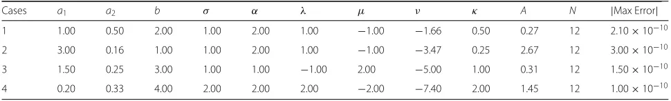
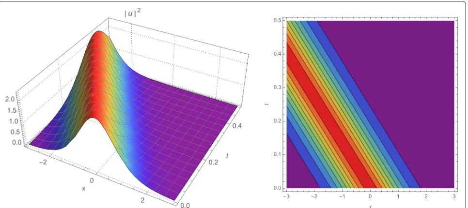
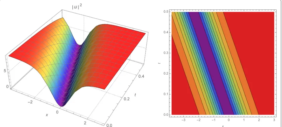
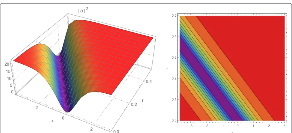
Table 1Bright optical solitons

Cases a1 a2 b σ α λ μ ν κ A N |Max Error|

1 1.00 0.50 2.00 1.00 2.00 1.00 −1.00 −1.66 0.50 0.27 12 2.10×10−10

2 3.00 0.16 1.00 1.00 2.00 1.00 −1.00 −3.47 0.25 2.67 12 3.00×10−10

3 1.50 0.25 3.00 1.00 1.00 −1.00 2.00 −5.00 1.00 0.31 12 1.50×10−10

4 0.20 0.33 4.00 2.00 2.00 2.00 −2.00 −7.40 2.00 1.45 12 1.00×10−10

Hence, Eq. (20) suggests the following iterative algorithm

u0(x,t)=f(x),

un+1(x,t)=L−1 1

sL{Run(x,t)+An(u0,u1,. . .,un)}

, n=0, 1, 2,. . .

(21)

Finally, after determining un’s, the N-term truncated

approximation of the solution is obtained as

uN(x,t)= N−1

n=0

un(x,t), N≥1. (22)

From this analysis it is evident that, the Adomian decom-position method, combined with the Laplace transform requires less effort in comparison with the traditional Adomian decomposition method. This method consider-ably decreases the number of calculations. In addition, Adomian decomposition procedure is easily established without requiring to linearize the problem.

Solution of the perturbed Fokas-Lenells equation by LADM

In this section, we outline the application of LADM to obtain explicit solution of Eq. (1) with the initial condi-tionsu(x, 0)=f(x), ux(x, 0)=g(x).

Let us consider the dimensionless form of the perturbed Fokas-Lenells equation Eq. (1) in an operator form

Lu(x,t)+Ru(x,t)+N1u(x,t)+N2u(x,t)+N3u(x,t)=0

(23)

where the notation N1u = −i|u|2(bu + iσux),

N2u = −λ(|u|2u)x and N3u = −μu(|u|2)x

symbol-ize the nonlinear term, respectively. The notationRu = −(αux+ia1uxx+ia2uxt) symbolize the linear

differen-tial operator andLu = ut simply means derivative with

respect to time.

The LADM represents solution as an infinite series of components given below,

u(x,t)= ∞

n=0

un(x,t). (24)

The nonlinear termsN1u,N2uandN3ucan be

decom-posed into infinite series of Adomian polynomials given by:

N1u= −i|u|2(bu+iσux)=

∞

n=0

Pn(u0,u1,. . .,un),

(25)

Fig. 1Dynamic evolution profile of|u|2_{via LADM (left) and contour plot of the wave amplitude of}_|_u_|2_{(right) for the values of the parameters used}

(4)

Fig. 2Dynamic evolution profile of_|u_|2_{via LADM (left) and contour plot of the wave amplitude of}_|_u_|2_{(right) for the values of the parameters used}

in case 2 with_|Max Error_{| =}3.0_×10−10

N2u= −λ

|u|2u_x= ∞

n=0

Qn(u0,u1,. . .,un), (26)

and

N3u= −μu

|u|2_x=

∞

n=0

Rn(u0,u1,. . .,un). (27)

HerePn,QnandRn are the Adomian polynomials and

can be calculated by the formula given by the Eq. (19), that is,

P0=N1(u0), Q0=N2(u0), R0=N3(u0),

and for everyn≥1 we have

Pn=

1 n

m i=1

n−1

k=0

(k+1)ui,k+1_∂∂ ui,0

Pn−1−k, (28)

(5)

in case 4 with|Max Error| =1.0×10−10

Qn=

1 n

m i=1

n−1

k=0

(k+1)ui,k+1_∂∂ ui,0

Qn−1−k, (29)

Rn=

1 n

m i=1

n−1

k=0

(k+1)ui,k+1_∂∂ ui,0

Rn−1−k. (30)

The first few Adomian polynomials are given by

P0= −ibu20u¯0,

P1= −2ibu0u1u¯0−ibu20u¯1,

P2= −2ibu0u2u¯0−ibu21u¯0−2ibu0u1u¯1−ibu20u¯2,

P3= −2ibu0u3u¯0−2ibu1u2u¯0−2ibu0u2u¯1−ibu21u¯1

−2ibu0u1u¯2−ibu20u¯3,

P4= −ibu¯0u22−2ibu0u¯0u4−2ibu¯0u1u3−2ibu0u¯1u3

−2ibu1u¯1u2+2u0u¯2u2−ibu21u¯2

−2ibu0u¯1u3−ibu20u¯4,

.. .

Q0= −(λ+μ)u20u¯0x,

Q1= −(λ+μ)

u2₀u¯1x+2u0u1u¯0x

, Q2=−(λ+μ)

u2₁u¯0x+u20u¯2x+2u0u1u¯1x+2u0u2u¯0x

,

Q3= −(λ+μ)

u2₁u¯1x+u20u¯3x+2u0u1u¯2x

+2u0u2u¯1x+2u0u3u¯0x+2u1u2u¯0x),

Q4= −(λ+μ)

u2₂u¯0x+u21u¯2x+2u0u1u¯3x+2u0u2u¯2x

+2u0u3u¯1x+2u0u4u¯0x+2u1u2u¯1x+2u1u3u¯0x),

.. .

R0=(σ −2λ−μ)u0u¯0u0x,

R1=(σ −2λ−μ)(u0u¯0u1x+u0u¯1u0x+u1u¯0u0x),

R2=(σ −2λ−μ) (u0u¯0u2x+u0u¯1u1x+u0u¯2u0x

+u1u¯0u1x+u1u¯1u0x+u2u¯0u0x),

+u0u¯3u0x+u1u¯0u2x+u1u¯1u1x+u1u¯2u0x

+u2u¯2u0x+u3u¯0u1x+u3u¯1u0x+u4u¯0u0x),

.. .

Table 2Dark optical solitons

Cases a1 a2 b σ α λ μ ν κ B N |Max Error|

5 2.00 0.25 1.00 −1.00 −2.00 1.00 −2.00 −2.33 1.00 1.68 12 2.50×10−10

6 1.50 0.20 −3.00 2.00 −1.00 0.33 0.50 −4.71 1.50 3.12 12 2.50×10−10

7 0.20 0.33 −4.00 2.00 2.00 2.00 −2.00 −7.40 2.00 1.15 12 1.00×10−10

(6)

Then, the Adomian polynomials corresponding to the nonlinear partNu=N1u+N2u+N3uare

A0= −ibu20u¯0−(λ+μ)u20u¯0x+(σ−2λ−μ)u0u¯0u0x,

A1= −2ibu0u1u¯0−ibu20u¯1−(λ+μ)(u20u¯1x+2u0u1u¯0x)

+(σ −2λ−μ)(u0u¯0u1x+u0u¯1u0x+u1u¯0u0x),

A2= −2ibu0u2u¯0−ibu21u¯0−2ibu0u1u¯1−ibu20u¯2

−(λ+μ)u2₁u¯0x+u20u¯2x+2u0u1u¯1x+2u0u2u¯0x

+(σ −2λ−μ)(u0u¯0u2x+u0u¯1u1x+u0u¯2u0x

A3= −2ibu0u3u¯0−2ibu1u2u¯0−2ibu0u2u¯1−ibu21u¯1

−2ibu0u1u¯2−ibu20u¯3−(λ+μ)(u21u¯1x+u20u¯3x

+2u0u1u¯2x+2u0u2u¯1x+2u0u3u¯0x+2u1u2u¯0x)

+(σ −2λ−μ)×(u0u¯0u3x+u0u¯1u2x+u0u¯2u1x

(7)

and so on for other Adomian polynomials.

By applying the Laplace transform with respect toton both sides of the Eq. (23) and using the linearity of the Laplace transform gives:

L{Lu(x,t)} = −L{Ru(x,t)} −L{N1u(x,t)}

−L{N2u(x,t)} −L{N3u(x,t)}.

(31)

Because of the differentiation property of Laplace trans-form, Eq. (31) can be written as

sL{u(x,t)} −u(x, 0)= −L{Ru(x,t)} −L{N1u(x,t)}

−L{N2u(x,t)} −L{N3u(x,t)}.

(32)

Thus,

L{u(x,t)} = 1

su(x, 0)− 1

s(L{Ru(x,t)} +L{N1u(x,t)} +L{N2u(x,t)} +L{N3u(x,t)}).

(33)

(8)

By substituting (24), (25), (26) and (27) into (33), we obtain

L

_∞

n=0

un(x,t)

=f(x)

s − 1 s L R ∞

n=0

un(x,t)

+L

_∞

n=0

Pn

+L

_∞

n=0

Qn

+L

_∞

n=0

Rn

.

(34)

Comparing both sides of the Eq. (34), the following rela-tions arise:

L{u0(x,t)} = f(x)

s (35)

L{u1(x,t)} = −

1

s(L{Ru0(x,t)} +L{P0} +L{Q0} +L{R0}) (36)

L{u2(x,t)}=−1

s(L{Ru1(x,t)}+L{P1}+L{Q1}+L{R1}).

(37)

In general, we get the following recursive algorithm

L{un+1(x,t)} = −

1

s(L{Run(x,t)} +L{Pn} +L{Qn} +L{Rn}), n≥1.

(38)

Finally, by applying inverse Laplace transformation we deduce the following recurrence formulas for each n = 0, 1, 2,. . .,

⎧ ⎨ ⎩

u0(x,t)=f(x), un+1(x,t)= −L−1

₁

sL{Run(x,t)+Pn(u0,. . .,un)

+Qn(u0,. . .,un)+Rn(u0,. . .,un)}

. (39)

Numerical simulations and graphical results We perform numerical simulations for bright and dark optical solitions.

Application to bright optical solitions

The result and the profile of four cases are shown in Table1and in Figs.1,2,3and4.

Application to dark optical solitions

The result and the profile of four cases are shown in Table2and in Figs.5,6,7and8.

Conclusions

This paper successfully studied FLE in polarization-preserving fibers by the aid of Laplace-Adomian decom-position scheme. The numerical scheme yielded bright and dark soliton solutions. The results thus appear with a complete spectrum of soliton solutions. Although sin-gular solitons is a third form of solitons that emerge

from this model, it does not provide any interest with any kind of numerical scheme. The results of the paper are truly encouraging to study the methodology fur-ther along. Later, this scheme will be applied to vec-tor coupled FLE that studies solitons in birefringent fibers. Further along the model will be extended to address WDM/DWDM/UDWDM topology numerically. Such studies are currently under way.

Abbreviations

DWDM: Dense wavelength division multiplexing; FLE: Fokas-lennels equation; GVD: Group velocity dispersion; IMD: Inter-modal dispersion; LADM: Laplace-adomian decomposition method; ND: Nonlinear dispersion; STD: Spatio-temporal dispersion; UDWDM: Ultra-dense wavelength division multiplexing; WDM: Wavelength-division multiplexing

Acknowledgments Not applicable.

Authors’ contributions

The original ideas and results emerged from discussions among all the authors. OGG wrote the manuscript with input from all authors. All authors read and approved the final manuscript.

Funding

The research work of the third author (MRB) was supported by the grant NPRP 8-028-1-001 from QNRF and he is thankful for it.

Availability of data and materials Not applicable.

Competing interests

The authors declare that they have no competing interests.

Author details

1_{Departamento de Matemáticas Aplicadas y Sistemas, Universidad Autónoma}

Metropolitana-Cuajimalpa, Vasco de Quiroga 4871, 05348, Mexico City, Mexico.2Department of Physics, Chemistry and Mathematics, Alabama A&M University, Normal, AL, Huntsville 35762, USA.3_{Department of Mathematics,}

King Abdulaziz University, 21589, Jeddah, Saudi Arabia.4Department of Mathematics and Statistics, Tshwane University of Technology, 0008, Pretoria, South Africa.5Science Program, Texas A&M University at Qatar, Doha, Qatar.

Received: 10 April 2019 Accepted: 28 May 2019

References

1. Biswas, A., Ekici, M., Sonmezoglu, A., Alqahtani, R. T.: Optical soliton perturbation with full nonlinearity for Fokas-Lenells equation. Optik.165, 29–34 (2018)

2. Biswas, A., Yildirim, Y., Yasar, E., Zhou, Q., Mahmood, M. F., Moshokoa, S. P., Belic, M.: Optical solitons with differential group delay for coupled Fokas-Lenells equation using two integration schemes. Optik.165, 74-86 (2018)

3. Biswas, A., Ekici, M., Sonmezoglu, A., Alqahtani, R. T.: Optical solitons with differential group delay for coupled Fokas–Lenells equation by extended trial function scheme. Optik.165, 102–110 (2018)

4. Jawad Mohamad, A. J., Biswas, A., Zhou, Q., Moshokoa, S. P., Belic M.: Optical soliton perturbation of Fokas-Lenells equation with two integration schemes. Optik.165, 111-116 (2018)

5. Biswas, A., Rezazadeh, H., Mirzazadeh, M., Eslami, M., Ekici, M., Zhou, Q., Moshokoa, S. P., Belic, M.: Optical soliton perturbation with Fokas-Lenells equation using three exotic and efficient integration schemes. Optik.165, 288-294 (2018)

(9)

7. Aljohani, A. F., Ebaid, A., El-Zahar, E. R., Ekici, M., Biswas, A.: Optical soliton perturbation with Fokas-Lenells model by Riccati equation approach. Optik.172, 741–745 (2018)

8. Biswas, A., Y&imath;ld&imath;r&imath;m, Y., Ya¸sar, E., Zhou, Q., Moshokoa, S. P., Belic, M.: Optical soliton solutions to Fokas-Lenells equation using some different methods. Optik.173, 21–31 (2018)

9. Arshed, S., Biswas, A., Zhou, Q., Moshokoa, S. P., Belic, M.: Optical solitons with polarization-mode dispersion for coupled Fokas-Lenells equation with two forms of integration architecture. Opt. Quant. Electron.50, 304 (2018)

10. Bansal, A., Kara, A. H., Biswas, A., Moshokoa, S. P., Belic, M.: Optical soliton perturbation, group invariants and conservation laws of perturbed Fokas-Lenells equation. Chaos, Solitons & Fractals.114, 275–280 (2018) 11. Krishnan, E. V., Biswas, A., Zhou, Q., Alfiras, M.: Optical soliton perturbation

with Fokas-Lenells equation by mapping methods. Optik.178, 104–110 (2019)

12. Arshed, S., Biswas, A., Zhou, Q., Khan, S., Adesanya, S., Moshokoa, S. P., Belic, M.: Optical solitons pertutabation with Fokas-Lenells equation by

exp(−φ(ξ))-expansion method. Optik.179, 341–345 (2019)

13. Bansal, A., Kara, A. H., Biswas, A., Khan, S., Zhou, Q., Moshokoa, S. P.: Optical solitons and conservation laws with polarization-mode dispersion for coupled Fokas-Lenells equation using group invariance. Chaos, Solitons & Fractals.120, 245-249 (2019)

14. González-Gaxiola, O., Biswas, A.: W-shaped optical solitons of Chen-Lee-Liu equation by Laplace-Adomian decomposition method. Opt. Quant. Electron.50, 314 (2018)

15. González-Gaxiola, O., Biswas, A.: Akhmediev breathers, Peregrine solitons and Kuznetsov-Ma solitons in optical fibers and PCF by Laplace-Adomian decomposition method. Optik.172, 930–939 (2018)

16. González-Gaxiola, O., Biswas, A.: Optical solitons with

Radhakrishnan-Kundu-Lakshmanan equation by Laplace-Adomian decomposition method. Optik.179, 434–442 (2019)

17. Fokas, A. S.: On a class of physically important integrable equations. Physica. D.87, 145–150 (1995)

18. Lenells, J.: Exactly solvable model for nonlinear pulse propagation in optical fibers. Stud. Appl. Math.123, 215-232 (2009)

19. Lenells, J., Fokas, A. S.: On a novel integrable generalization of the nonlinear Schrödinger equation. Nonlinearity.22, 11-27 (2009) 20. Yang, C., Liu, W., Zhou, Q., Mihalache, D., Malomed, B. A.: One-soliton

shaping and two-soliton interaction in the fifth-order variable-coefficient nonlinear Schrödinger equation. Nonlinear Dyn.95, 369–380 (2019) 21. Triki, H., Zhou, Q., Liu, W.: W-shaped solitons in inhomogeneous

cigar-shaped Bose-Einstein condensates with repulsive interatomic interactions. Laser Phys.29, 055401 (2019)

22. Yang, C., Wazwaz, A. M., Zhou, Q., Liu, W.: Transformation of soliton states for a(2+1)dimensional fourth-order nonlinear Schrödinger equation in the Heisenberg ferromagnetic spin chain. Laser Phys.29, 035401 (2019) 23. Aouadi, S., Bouzida, A., Daoui, A. K., Triki, H., Zhou, Q., Sha, Liu.: W-shaped,

bright and dark solitons of Biswas-Arshed equation. Optik.182, 227–232 (2019)

24. Zhang, Y., Yang, C., Yu, W., Mirzazadeh, M., Zhou, Q., Liu, W.: Interactions of vector anti-dark solitons for the coupled nonlinear Schrödinger equation in inhomogeneous fibers. Nonlinear Dyn.94, 1351–1360 (2018) 25. Wazwaz, A. M.: A new algorithm for calculating Adomian polynomials for

nonlinear operators. Appl. Math. Comput.111(1), 33-51 (2000) 26. Duan, J. S.: Convenient analytic recurrence algorithms for the Adomian

polynomials. Appl. Math. Comput.217, 6337-6348 (2011) 27. Duan, J. S.: New recurrence algorithms for the nonclassic Adomian

polynomials. Appl. Math. Comput.62, 2961-2977 (2011)

Publisher’s Note