Reconsidering No-Go Theorems from a Practical
Perspective
∗
,†
Michael E. Cuffaro
Ludwig-Maximilians-Universität München, Munich Center for Mathematical Philosophy
Abstract
I argue that our judgements regarding the locally causal models which are compatible with a given quantum no-go theorem implicitly depend, in part, on the context of inquiry. It follows from this that certain no-go theorems, which are particularly striking in the traditional foundational context, have no force when the context switches to a discussion of the physical systems we are capable of building with the aim of classically reproducing quantum statistics. I close with a general discussion of the possible implications of this for our understanding of the limits of classical description, and for our understanding of the fundamental aim of physical investigation.
1
Introduction
Bell’s inequalities, and results like them, are often presented as ‘no-go theorems’ in the philosophical and physical literature. They are portrayed as demonstrating, for instance, that no ‘locally causal’ (Bell, 2004 [1990], §7) description of the em-pirically confirmed predictions of quantum mechanics is possible, that one cannot ascribe ‘elements of reality’, in EPR’s sense (Einstein, Podolsky, & Rosen, 1935), to quantum systems consistently with such predictions, and so on. As I will argue below, however, thinking of Bell’s and related results in this way—without further qualification—can be misleading, for they are not no-go theorems per se. Rather,
∗Note: this is the submitted version of an article that is to appear inThe British Journal for the
Philosophy of Science, published byOxford University Press. Changes have been made to this article since it was submitted for publication. These improvements are mostly clarificatory in nature and do not substantially modify the structure or argument of the paper. They are primarily found in §6 (which has been expanded), and at the end of §4. When citing this paper, please refer to the published version.
†Thanks to Sam Fletcher for his helpful comments and suggestions on an earlier draft of this
they are best understood as establishing certain general constraints on locally causal descriptions of joint measurement outcomes. In order to turn Bell’s and similar re-sults into no-go theorems, one must do more than just state them. One must also interpret them in the context of the question one takes them to be informing.
Associated with a given context are a number of additional constraints, according to which we judge a locally causal description to be either plausible or implausible in that context. Normally these ‘plausibility constraints’ are left unstated, and this is mostly harmless most of the time, for the relevant context is usually understood to be what I will below be calling the ‘theoretical’. Here the question we take Bell’s and related results to be answering is the question of whether there is an alternative locally causal description of the natural world that can recover the confirmed pre-dictions of quantum mechanics. The set of plausibility constraints on locally causal descriptions—or anyway the general character of such constraints—in the context of this question is implicitly understood by all.
Bell’s and related results are relevant to other contexts having to do with phys-ical systems as well, however. In particular, in what I will below be calling the ‘practical’ context, we are not concerned with alternative theories of the natural world, classical or otherwise. What we are rather concerned with are the kinds of physical systems that we can build in order to recover a particular probability dis-tribution or set of measurement outcomes. As I will describe in more detail below, the plausibility constraints we impose on locally causal descriptions in this context are importantly different from those we impose in the theoretical context. Thus the kinds of locally causal description we think are worth considering as alternatives to quantum description in the former context will be different from the kinds of locally causal description we think are worth considering in the latter.
This has interesting and important implications. Cuffaro (forthcoming) has ar-gued that distinguishing between these two contexts can help us to understand the way certain physical resources are taken advantage of in the science of quantum computation. The present article builds upon Cuffaro’s work.1 In it I will argue that making this distinction can help us to better understand the relative power and scope of no-go theorems, and in so doing provide us with a new point of view from which to consider the fundamental differences between classical and quantum systems in general.
Consider, in particular, Greenberger, Horne, & Zeilinger (GHZ)’s so-called ‘all-or-nothing’ equality (Greenberger et al., 1989). It is typical in the philosophical and foundational literature to see this equality referred to as a more powerful refuta-tion of local causality than Bell’s own statistical inequality. The reason for this is that, while a violation of the GHZ equality can in principle be shown with a single quantum experiment, a violation of Bell’s requires repeated quantum experiments to demonstrate (and even then only with increasing, but never absolute, confidence). Greenberger, Horne, Shimony, & Zeilinger (1990, p. 1131), for example, write: “This incompatibility with quantum mechanics is stronger than the one previously
1To my knowledge, Cuffaro is the first to explicitly make this distinction. The general idea,
revealed for two-particle systems by Bell’s inequality, where no contradiction arises at the level of perfect correlations.” Clifton, Redhead, & Butterfield (1991, p. 174) likewise write, of their improvement on the original GHZ proof, “[o]ne difference between Bell’s theorem and ours is that his yields a statistical contradiction, whereas ours leads to an algebraic one. So in one respect, our conclusion is stronger.”2 Mer-min, for whom the GHZ proof is “spectacular” (1993, p. 810), enthusiastically agrees: “[t]his is an altogether more powerful refutation of the existence of ele-ments of reality than the one provided by Bell’s theorem ...” (1990, p. 11). And Maudlin concurs: “the GHZ scheme brings home the problem for locality all the more sharply” (Maudlin, 2011, p. 26). So, also, does Vaidman: “The GHZ proof is the most clear and persuasive proof of nonexistence of local hidden variables” (1999, p. 615). Indeed, for Vaidman, the significance of the GHZ proof is quite profound: “analysis of the GHZ work led me to accept the bizarre picture of quantum reality given by the many worlds interpretation, ...” (ibid., p. 616). Vaidman is not alone in taking the GHZ equality as a starting point from which to consider the question of the interpretation of quantum mechanics (e.g., see Hemmo & Pitowsky, 2003).
There is nothing inappropriate about this kind of talk, so long as it is confined (as it presumably is for the above authors) to what I have above called the theoretical context. When we move, however, from the theoretical to the practical context, then interestingly, the above statements are false. As I will elaborate upon in more detail below, in the practical context, the all-or-nothing GHZ theorem loses its force. In the practical context, in fact, it is only statistical inequalities which can legitimately be turned into no-go theorems (although, also interestingly, one must indeed go be-yond Bell’s theorem, and its associated bipartite entangled states, to entangled states of multipartite systems in order to show this). From this we may say that from the ‘absolute’ point of view—i.e. when considering the limits of plausible classical phys-ical description as such—it is statistphys-ical inequalities, rather than the all-or-nothing GHZ, which are more powerful in the sense alluded to by the authors above, for sta-tistical inequalities—and not the all-or-nothing GHZ—allow us to see that there are quantum statistics that even we can’t plausibly build classical systems to reproduce.
The sections of this paper are the following: in §2 I review CHSH’s variant of Bell’s inequality as well as the GHZ equality. In §3 I describe some schemes by which one could simulate, using a classical computer, some of the statistics associated with Bell and GHZ states. In §4 the meaning of the term “classical computer simulation” is reflected upon. The implications of these reflections for our understanding of the relative strength of statistical no-go theoremsvis á vis the all-or-nothing GHZ theo-rem are considered in §5. Finally, their general implications for our understanding of the limits of classical description, and for our understanding of the fundamental aim of physical investigation, are considered in §6.
2Note that, as this quote hints at, Clifton et al. do not argue that the GHZ proof is stronger than
2
‘No-Go’ Results
2.1
The CHSH inequality
Consider the singlet state, |Ψ−〉 = 1/p2(| ↑〉| ↓〉 − | ↓〉| ↑〉) of two spin-1⁄2 particles. For a system in this state, the expectation value for joint experiments on its two subsystems is given by the following expression:
〈σm⊗σn〉=−mˆ ·nˆ=−cosθ. (2.1)
Hereσm,σn represent spin-mand spin-nexperiments on the first (Alice’s) and sec-ond (Bob’s) subsystem, respectively, with ˆm, ˆnthe unit vectors representing the ori-entations of their two experimental devices, and θ the difference in these orienta-tions.
It is well known that it is not possible to provide an alternative theory accounting for the predictions associated with this state if that theory makes the very reasonable assumption that the probabilities of local experiments on Alice’s (and likewise Bob’s) subsystem are completely determined by her local experimental setup together with a shared hidden variableλtaken on by both subsystems at the time the joint state is prepared (i.e. while A and B are still physically interacting). For, given such a theory, we will have that
〈σm⊗σn〉λ =〈Aλ(mˆ)×Bλ(ˆn)〉, (2.2)
whereAλ(mˆ)∈ {±1},Bλ(nˆ)∈ {±1}represent the results, given a specification of the hidden variableλ, of spin experiments on Alice’s and Bob’s subsystems. But consider the following expression relating the expectation values of different combined spin experiments on Alice’s and Bob’s subsystems for arbitrary directions ˆm, ˆm′, ˆn, ˆn′:
CHSH: |〈σm⊗σn〉+〈σm⊗σn′〉|+|〈σm′⊗σn〉 − 〈σm′⊗σn′〉|.
When (2.2) holds, one can show that
CHSH≤2. (2.3)
The ‘CHSH inequality’ (Clauser, Horne, Shimony, & Holt, 1969) is one of a family of similar expressions, known collectively as the ‘Bell inequalities’,3 which must be satisfied by locally causal theories aiming to account for the statistics associated with combined spin measurements.
The statistical predictions of quantum mechanics violate the CHSH inequality for some experimental configurations. For example, let the system be in the singlet state and let the unit vectors ˆm, ˆm′, ˆn, ˆn′ (taken to lie in the same plane) have the orientations 0,π/2,π/4,−π/4 respectively. The differences,θ, between the differ-ent oridiffer-entations (i.e., ˆm−nˆ, ˆm−nˆ′, ˆm′−nˆ, and ˆm′−ˆn′) will all be in multiples of
π/4 and we will have, from (2.1):
|〈σm⊗σn〉+〈σm⊗σn′〉|+|〈σm′⊗σn〉 − 〈σm′⊗σn′〉|=2 p
26≤2.
We normally conclude from this that the predictions of quantum mechanics for arbitrary orientations ˆm, ˆm′, ˆn, ˆn′, cannot be reproduced by any alternative theory in which all of the correlations between subsystems are due to a common parame-ter endowed to them at state preparation. But note that these predictions can be reproduced by such a hidden variables theory for certain special cases. In particu-lar, the inequality is satisfied by quantum mechanics when ˆmand ˆn, ˆm and ˆn′, ˆm′
and ˆn, and ˆm′and ˆn′ are all oriented at angles with respect to one another that are given in multiples ofπ/2. Note that these are the cases for which Eq. (2.1) predicts perfect correlation (θ =π), perfect anti-correlation (θ =0), or no correlation at all (θ=π/2).
For example, let λ determine Alice’s and Bob’s measurement results in the fol-lowing way:
Aλ(mˆ) =sign(mˆ ·λˆ),
Bλ(ˆn) =−sign(ˆn·λˆ), (2.4)
where sign(x) is a function which returns the sign (+ or -) of its argument. The reader can verify that (2.4) will recover all of the statistical predictions associated with the singlet state (2.1) just so long as the difference in orientation between ˆm
and ˆnis some multiple ofπ/2 (Bell, 2004[1964], p. 16).
2.2
The GHZ equality
We have just seen that the statistics associated with the singlet state for measurement angles differing in proportion to π/2 are reproducible in a local hidden variables theory such as (2.4). But this is not true for every entangled state. In particular, for a system of three spin-1⁄
2particles in the state:
|GHZ〉= | ↑〉a| ↑〉b| ↑〉cp− | ↓〉a| ↓〉b| ↓〉c
2 , (2.5)
one can, by considering measurements of Pauli observables (σx, σy, σz),4 demon-strate a conflict between the predictions of quantum mechanics and those of a suit-ably local hidden variables theory. Note that the respective orientations of different ends of an experimental apparatus set up to conduct an experiment involving Pauli observables on a combined system will never differ by anything other than an angle proportional toπ/2.
To see how this conflict arises, note that in the GHZ state,5 the eigenvalues as-sociated withσx and σy observables on individual subsystems are (as always)±1, while each of the tripartite observables,
σax ⊗σby ⊗σcy, σay⊗σxb⊗σcy, σay⊗σby ⊗σcx (2.6)
(which, as the reader can verify, are compatible) takes the eigenvalue 1; i.e.,
v(σax⊗σby ⊗σcy) =v(σay⊗σxb⊗σcy) =v(σay ⊗σby ⊗σcx) =1. (2.7)
Thus preparing a tripartite system in the state (2.5) will yield correlations, ex-pressed by (2.7), between the results of certain measurements at the sitesa, b, and
c. Since a, b, and c may in general be quite distant from one another, it is reason-able to assume, if one is reasoning classically, that the subsystems measured at those sites became correlated while they were still in physical interaction with one another (i.e., at state preparation) by way of some shared common cause (represented by a variable λ). Thus, at the time of measurement, nothing further should influence an individual outcome aside from the local properties of the experimental setup at a site and of the particle being measured there. Thus the results of the combined measurements (2.7) will be factorisable givenλ; i.e.,
v(σax⊗σby ⊗σcy) =1=v(σax)×v(σyb)×v(σcy),
v(σay ⊗σbx ⊗σcy) =1=v(σay)×v(σxb)×v(σcy),
v(σa y ⊗σ
b y⊗σ
c
x) =1=v(σ a
y)×v(σ b
y)×v(σ c
x). (2.8)
But this cannot be. Multiplying the right hand sides of (2.8), and using the fact that v(σa
y)
2 = v(σb y)
2 = v(σc y)
2 = 1, we have it that v(σa
x)×v(σ b
x)×v(σ c x) = 1,
which in turn (given factorisability) implies that
v(σax⊗σbx⊗σcx) =1. (2.9)
Quantum mechanically, however, if we take the product (we can since they are com-patible) of the observables in (2.6), then since σxσy = iσz = −σyσx, σxσz =
−iσy =−σzσx,σyσz =iσx =−σzσy,σxσx =σyσy =σzσz= I, this must yield:
(σa x ⊗σ
b y⊗σ
c y)(σ
a y⊗σ
b x⊗σ
c y)(σ
a y ⊗σ
b y⊗σ
c x)
= −σax ⊗σbx ⊗σcx. (2.10)
Since each of the observables in (2.6) takes the eigenvalue 1, this implies that
v(σax ⊗σxb⊗σcx) =−1. (2.11)
Thus (2.9), which we were led to through the assumption of factorisability (2.8), contradicts the (empirically confirmed) predictions of quantum mechanics (2.11). We conclude, therefore, that the correlations expressed by (2.7) do not admit of a locally causal description.
3
Classically simulating quantum statistics
The results just described have unquestionably deepened our understanding of the implications of our experience with quantum phenomena. Yet the proper analysis and precise significance of these implications for our understanding of nature has, unsurprisingly, been hotly debated both by philosophers and physicists.6 We will not
σx σy σz
I
a b c
−R2R3 R2 R3
−iR1R2R3 iR1R2 iR1R3 R1 R1 R1
1 1 1
.
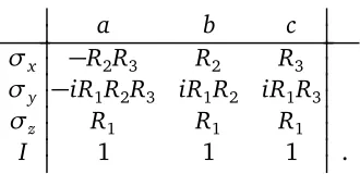
Table 1: A scheme for reproducing all of the Pauli measurement statistics associated with the tripartite GHZ state.
engage directly in those debates here. We will rather ask ourselves a different (but as we will see later, not unrelated) question: (i) could one build a classical machine to simulate the quantum measurement statistics described above (and if so, how)? If the answer is yes, then (ii) are there any quantum correlations that cannot be so simulated, or is it the case that one can build classical systems to reproduce every possible quantum mechanical correlational effect?
As it turns out, this is, in fact, an active area of research, and as we will see shortly, we can indeed give an affirmative answer to question (i). Later, in §4, we will consider the philosophical significance of this. In particular we will see (in §5) that it forces us to qualify some of the conclusions we made in §2. In the process we will answer question (ii).
3.1
GHZ statistics
Consider, first, the case of GHZ correlations.7 Table 1 depicts a scheme for reproduc-ing all of the Pauli measurement statistics associated with the state (2.5).
In the table,a, b, andc refer to the three subsystems of the system. σx,σy,σz, andI are the Pauli spin operators. The shared variablesR1,R2, andR3are values of
±1 that are assigned to the various subsystems at state preparation through some sequence of local interactions. It is assumed that these variables possess determinate values prior to measurement but that these values are completely ‘hidden’ in the sense that they can only be revealed by measurement, or what amounts to the same thing: two identical state preparations will in general yield (with equal likelihood) different values ofR1 (likewise forR2 andR3).8
To determine the outcome of a combined Pauli measurement on the system, one multiplies the entries of the table corresponding to the measurements performed on each subsystem, discarding any remaining unsquared i’s. For example, a mea-surement of σy on subsystem a is equivalent to σy ⊗I ⊗I. The result is given by −iR1R2R3, which, dropping the unsquared i, yields −R1R2R3 = ±1 with equal
7What follows is a summary of the model given in more detail in (Tessier, 2004; Tessier, Caves,
Deutsch, & Eastin, 2005).
8Note that no such interpretation ofR
1,R2, andR3is given in either (Tessier, 2004) or (Tessier
likelihood. Measuringσy⊗σx⊗σy, on the other hand, will yield
v(σy ⊗σx ⊗σy) =−iR1R2R3R2iR1R3=−i2R12R22R23=1 (3.1)
with certainty. And so, on. It is easy to verify that Table 1’s predictions for every combined Pauli measurement match up with those of quantum mechanics. And like those of quantum mechanics, Table 1’s predictions for combined Pauli measurements on the GHZ state are not factorisable, since, for example,
v(σy⊗I⊗I)×v(I⊗σx ⊗I)×v(I ⊗I⊗σy) =−R1R2R3R2R1R3=−1, (3.2)
in contradiction with (3.1). The instances of i in the table are the analogue of quantum mechanical ‘nonlocal’ influences.
With only very minor tweaking, however, one can build a model similar to the one represented in Table 1, in which the resulting correlations are both factorisable and consistent with all of the predictions of quantum mechanics for these measure-ments. Our tweak will be that we will allow the parties to classically signal to one another as follows. Bob (measuring b) and Alice (measuring a) will agree that he will send her a single classical bit indicating whether or not he performed aσy mea-surement on his subsystem. Upon receipt of this bit, Alice should flip the sign of her local outcome if either she or Bob (or if both of them) measuredσy. Thus instead of (3.2) we will have:
v(σy ⊗I⊗I)×v(I⊗σx⊗I)×v(I⊗I⊗σy) =R1R2R3R2R1R3=1, (3.3)
in agreement with (3.1). Note that this result is consistent with each of the three measurements σy ⊗I ⊗I, I ⊗σx ⊗I, I⊗I ⊗σy, for each of them separately will yield a value of±1 with equal probability.
This small addition—a single bit of classical communication—suffices to make the outcome of every joint measurement of Pauli observables factorisable in the model. The scheme generalises. For ann-partite system in the GHZ state 1/p2(| ↑〉⊗n±
| ↓〉⊗n), only n
−2 bits of classical communication are required. The same is true, moreover, not only forn-partite GHZ states, but also for anyn-partite state in which each superposition term is expressible as a product of Pauli eigenstates (details are given in Tessier 2004).
One can imagine building a classical computational system, made up of smaller spatially separated computational subsystems, utilising a small amount of classical communication as described above, to instantiate the description given in Table 1. This is the sense in which one may say that the correlations between the results of Pauli measurements on systems in the GHZ state are ‘efficiently classically simulable’. I will elaborate upon this in more detail in §4. But let us first consider how to simulate measurement statistics on a system in the singlet state.
3.2
Singlet statistics
As we saw earlier (2.4), Bell himself provided a local hidden variables description to account for Pauli measurement statistics in the singlet state.9 Presumably, we could
9The theory given in (2.4) applies not just to Pauli measurements, of course, but more generally,
build a classical computer to instantiate that description. Thus Pauli measurements on the singlet state are efficiently classically simulable in this sense. In this case no communication is needed, in fact. This is evident from (2.4). It also follows from the fact that Pauli measurement statistics on anyn-partite state, whose superposition terms are expressible as products of Pauli eigenstates, can be simulated usingn−2 bits. The singlet state is one such state for which n= 2. Thus for the singlet state, Pauli measurements can be simulated using 2−2=0 bits of communication.
It turns out that for the singlet state, we can simulate far more than just Pauli measurements if we allow ourselves only a single additional bit. Astoundingly, we can actually recover the statistics associated with arbitrary projective measurements by using the following method (Toner & Bacon, 2003). Randomly choose, inde-pendently, two unit vectors ˆλ1 and ˆλ2. At state preparation, share them with Al-ice and Bob, and instruct them to take their particles with them to separate dis-tant locations. Once there, have Alice measure her particle along the direction ˆm, and output the result A = −sign(mˆ ·λˆ1). Have her then send a single classical bit
c=sign(mˆ·λˆ1)×sign(mˆ·λˆ2) =±1 to Bob, who finally measures along ˆnand outputs the resultB=sign[ˆn·(λˆ1+cλˆ2)].
4
What is a classical computer simulation?
We have just seen how to, using only a few additional resources, classically simulate the quantum measurement statistics described in §2. We saw, specifically, that only a single bit is needed to recover the statistics associated with arbitrary projective measurements on the singlet state, and that onlyn−2 bits are needed to recover the statistics associated with Pauli measurements on n-partite GHZ states. Let us now reflect on this. To begin with, let us try and explicate somewhat more precisely what is meant by the statement that a particular set of quantum correlational statistics has been ‘classically simulated’.
What is a classical computer simulation, then? Most obviously, perhaps, we may say, to start with, that a classical computer simulation is something performable by a classical computer. Let us consider what is meant by the latter. A classical computer, whatever else it is, is a classical physical system, i.e., a system which can be given a classical physical description. Some of the characteristics of classical description are the following. First, a complete classical description of a system, which in general will consist of many subsystems, is always separable into complete descriptions of those individual subsystems. Second, a classical description of the interactions between a system’s subsystems will not violate classical physical law. For instance, the speed by which such interactions propagate should be less than or equal to the speed of light.10 Third, and importantly, the behaviour of classical systems is always describable in principle in terms of local causes and effects, in the metaphysically deflationary sense explicated by Bell (2004[1990]). Thus, while a classical system might evince certain correlations between experimental results on
experimental apparatus differ in proportion toπ/2.
10I am taking ‘classical’ in the sense in which it is typically used in discussions of quantum
its various subsystems—which, in general, can be quite distant from one another— since the system is classical, these correlations will always be describable as arising from a common source situated in the intersection of the prior light cones of the associated measurement events. These correlations, once we take into account their common causes, are always, that is, factorisable. Classical systems do not violate Bell (or GHZ, or similar) inequalities. Classical computer simulations, therefore, which are run on classical computers, which are instantiated by classical physical systems, do not either.
This is perfectly obvious. And yet it might still strike one as strange. The results of, say, a Bell experiment seem to be evidence for some sort of influence (even if only benign) between the spatially separated subsystems of entangled systems, and we usually take this to demonstrate that quantum systems are ‘nonlocal’ (or perhaps ‘nonseparable’) in some sense (see, e.g., Maudlin 2011); i.e., we take such influ-ences to demonstrate that no locally causal description—no ‘local hidden variables theory’—of the outcomes of these experiments is possible. But the influence of one spatially separated subsystem on another is precisely what we find in the protocols designed to reproduce these outcomes described in §3. And yet these are locally causal descriptions. How can this be?
A way of resolving this tension has been convincingly provided by Cuffaro (forth-coming). I will not reproduce that discussion in its entirety here, but rather only sum-marise the main points emerging from it that are relevant to our own investigation (for a full elaboration and defense of these points, see the aforementioned article). Cuffaro argues that when we make a judgement to the effect that no local hidden variables theory is capable of recovering the quantum mechanical predictions asso-ciated with a Bell experiment, implicit in this judgement is a set of constraints upon the kinds of local hidden variables theory that we are willing to entertain. To put it another way: with a little imagination it is always possible to conceive of loopholes to the Bell inequalities, but only some of these loopholes—the plausible ones—are worth the bother of trying to close. This means, however, that a conclusion such as “no (plausible) hidden variables theory of typeX is able to reproduce the experi-mental predictions of quantum mechanics with respect to preparation procedureY” cannot really be forced on the basis of Bell’s (or a similar) (in)equality alone. Strictly speaking, to force such a conclusion, what one means by ‘plausible’ must be spelled out first.
Usually, of course, we do not really need to be explicit. There is a set of criteria by which we mark a hidden variables theory as plausible which is implicitly understood by everyone. This set includes such things as consistency with our other theories of physics, with the body of our experiential knowledge in general; we expect a can-didate local hidden variables theory not to be conspiratorial, and so on. These and other plausibility constraints are associated with what Cuffaro calls the ‘theoretical’ context, wherein we take Bell’s and related results to enlighten questions such as ‘is there an alternative (locally causal) description of the natural world that can recover the confirmed predictions of quantum mechanics?’
wherein our concern is not with alternative theories of the natural world, but rather with what we are capable of building with the aim of (classically) reproducing the statistical predictions of quantum mechanics. In the practical context we are con-cerned, in other words, not with ‘local hidden variables’ descriptions of the natural world, but with ‘practical classical’ descriptions of machines that are possible for us to build to achieve particular ends (in the sequel I will be using, with Cuffaro, the generic term ‘locally causal description’ to refer to both).
Now consider the two classical schemes for simulating quantum statistics de-scribed in §3. Either of these can be thought of as an alternative locally causal description of the observation of a given set of measurement statistics in the follow-ing way. Begin by askfollow-ing what we really need to recover in an alternative locally causal description of a combined measurement outcome. The answer invariably will be: just the actual observation of the combined outcome itself. What I mean is this: although quantum mechanics posits its own particular dynamics—involving, for example, the state collapse of a subsystem of a Bell pair upon the measurement of the other subsystem—an alternative description of the events leading up to the observation of a combined measurement outcome can in principle disagree entirely with the quantum mechanical dynamical description. All that an alternative locally causal description needs to be faithful to in principle is our actual observation of the combined result.
Importantly, in order to be in a position to assert that one has observed a com-bined measurement outcome, one must first have comcom-bined the individual mea-surement outcomes; Alice and Bob must report their results to Candice (or to each other) over tea or by telephone or in writing or by using some other physical means. This is absolutely necessary and there simply is no escaping it. While these re-sults are being brought together, however, Alice and Bob have time to (conspiratori-ally) exchange—at subluminal velocity—a series of finite signals with one another, and thus coordinate—and if necessary, ‘correct’—their individual measurement out-comes in the manner described in §3. But notice now that with respect to the ob-servation of the combined measurement outcome—which, to reiterate, is ultimately what we are required to explain—all of this conspiratorial signalling will have oc-curred in its past light cone. It is thus part of a posited state preparation—a common cause—for that combined outcome and it thus comprises part of a classical, locally causal, alternative description of that combined outcome (see figure 1).
de-Figure 1: A conceivable explanation of the observation of the result of a joint experimental outcomeABwhich posits local (conspiratorial) influences interacting within regionC. This figure is adapted from Cuffaro (forthcoming).
fined naturalistically—i.e. by appealing to our best scientific theory of the subject: computational complexity theory.
To illustrate: imagine someone, call him Ray, attempting to convince you that a large black box sitting in a hangar at the airport is a quantum computer. Suppose that he either cannot or will not open the box, but that he rather attempts to convince you of this by having the computer run a calculation whose result depends (according to him) on the prior generation of a GHZ state. Now if you are skeptical of this claim, it will then be incumbent upon you to produce an alternative classical description— a blueprint, say—of the goings on within the box which explain your observations in the hangar. If, however, the best that you can do is specify a classical model for your observations that requires an infinite—or anyway some ‘enormous’—number of additional resources as compared to a quantum model, then in that case Ray may legitimately dismiss your objection, for it is implausible, he will say, that he or anyone could have built a machine conforming to your description. On the other hand if you can specify a machine whose description requires only ‘a few’ additional resources, in the manner of §3, then your skepticism is justified unless Ray provides you with additional evidence for his claim.11
Now in complexity theoretic terms, to solve a problem using ‘an enormous’ num-ber of resources means that these resources are exponential with respect to the size of the input to the problem,n; i.e. on the order ofkn. ‘A few’ resources, in contrast, are at most polynomial with respect ton; i.e., on the order ofnk.12 The protocols de-scribed in §3 require only a few additional resources to implement in this sense. In particular they require a number of additional resources that is only linear inn. For this reason, they and other efficient simulations of quantum measurement statistics may be thought of as alternative locally causal descriptions of those measurement
11This last qualification is important. Presumably if the box were open, for instance, there would
be ways to test for and close your loophole, at least in this simple scenario. This does not affect the conceptual point being made here, however.
12For a good and thorough text on the subject of computational complexity, consult Papadimitriou
statistics that are plausible in the practical context.13
5
Comparing the all-or-nothing GHZ with statistical
(in)equalities
We saw in §3.2 that if we would like to classically simulate the measurement statis-tics associated with Pauli measurements on a system in the singlet state, we can do so without the aid of any classical communication. To recover the statistics for arbitrary measurements, on the other hand, we require a single classical bit propa-gated at subluminal speed. In §3.1 we saw that recovering the statistics associated with Pauli measurements on a system in a GHZ state requires only a number of addi-tional resources that is linear in the number of systems,n. All of these measurement statistics are plausibly recoverable, therefore, in the practical context.
What if we would like to recover the statistics associated with arbitrary measure-ments on a system in a GHZ state? Unfortunately, unlike the singlet and other Bell states, it does not seem likely that we could plausibly do so. Tessier (2004, p. 116) notes that the number of classical bits required to model the quantum mechanical predictions associated with arbitrary projective measurements on n-partite states (forn ≥ 3) in a model like the one pictured in Table 1 is likely to be unbounded. This is consistent with other results due to Jozsa & Linden (2003), and to Abbott (2012), who show (using different methods) that for systems in pure states, an ex-ponential speed up of quantum over classical computation is possible only when one has available multipartite entanglement with a number of systemsn≥3.
Returning now to the GHZ argument which we discussed in §2.2. As is evident from some of the quotations we surveyed in §1, it is hard to overestimate the impact that the GHZ proof has had upon the physical and philosophical communities. To quote Mermin at length:
This is an altogether more powerful refutation of the existence of ele-ments of reality than the one provided by Bell’s theorem for the two-particle EPR experiment. Bell showed that the elements of reality in-ferred from one group of measurements are incompatible with the statis-tics produced by a second group of measurements. Such a refutation cannot be accomplished in a single run, but is built up with increasing confidence as the number of runs increases[...] In the GHZ experiment, on the other hand, the elements of reality require a class of outcomes to occurallof the time, while quantum mechanicsneverallows them to occur (Mermin, 1990, p. 11).
As we saw earlier, however, before one can properly make statements like this one concerning the relative power of the Bell and GHZ (in)equalities, one must first be clear on the context in which such a statement is being made. From a theoretical
13It must not be forgotten, of course, that at least in the case of GHZ states, it is only the
point of view it may be that the GHZ argument is more powerful than Bell’s in the above sense. Thus I take no issue with Mermin’s statement as long as it is qualified in this way, as I assume it implicitly is for Mermin. This said, in the practical context, Mermin’s statement is actually false. For from a practical point of view, both the Bell and GHZ (in)equalities are equally weak, in the sense that plausible alternative locally causal descriptions can be provided to account for the associated statistics in both cases.
The contrast being drawn in the quote above, however, and in the statements of the other philosophers and physicists cited in §1, is not specifically between the results of Bell and GHZ. It is rather between the GHZ equality insofar as it is an all-or-nothing result, and Bell’s inequality insofar as it is a statistical result. But as we have seen, it is quite easy to recover the statistics associated with Pauli measurements on the GHZ state—the measurements for which an all-or-nothing equality can be proved—in the practical context. In order to use the GHZ state as the basis for a
bona fideno-go theorem in this context, one must consider measurements outside of the Pauli group, for the statistics associated with these measurements cannot be plausibly recovered in a locally causal model in this context. Once one does so, however, the ensuing correlations between individual measurement results will no longer be strict but probabilistic. Thus it is statistical results, rather than the all-or-nothing GHZ, which are more powerful in the practical context.
6
General Discussion
We have chosen to call classical computer simulations of quantum mechanical corre-lational statistics locally causal alternative descriptions of those correcorre-lational statis-tics. This is not the way it is normally put in the quantum information literature. What is normally claimed for these schemes is rather that they quantify—in terms of the number of classical bits required to reproduce them—the departure from clas-sicality of quantum correlations (see, e.g., Rosset, Branciard, Gisin, & Liang, 2013). While this way of framing their significance is certainly not incorrect (and it is certainly, moreover, useful), from a more philosophical point of view it is preferable to, so to speak, call a spade a spade. As the example above involving the black box in the hangar makes clear, a plausible description of a locally causal computer simulation of a class of quantum phenomena is of the same general kind as a plau-sible locally causal theoretical description of a class of quantum phenomena. Both kinds of description represent alternative plausible stories one can put forward if one is skeptical regarding the quantum mechanical description of some set of ob-servations. The essential difference between the theoretical and practical contexts lies in the different presuppositions we make concerning the origin of the physical systems under consideration in each case. In the practical context we presuppose that a particular system has been designed and built by some rational agent for a particular purpose. We do not presuppose nature to be purposeful in this way in the theoretical context.14
14I am not expressing a theological opinion with this statement. I mean only that we do not
Additionally, calling a spade a spade helps us to understand one reason why the practical context is—or anyway should be—interesting from a philosopher of physics’ point of view. Indeed, the reader may have been wondering why she should care at all about the practical context—why a philosopher of physics should care for anything but the correct theory of the natural world and for its deeper consequences for our fundamental understanding of the ontology of that world. To help appreci-ate why we should care, imagine if it were possible to easily build classical machines to reproduce the statistics associated with every quantum mechanical measurement, regardless of the state and the number of systems such a measurement were per-formed upon. If this were possible it would surely be of immense philosophical in-terest, for it would signify that we can build classical physical systems to reproduce every observable quantum mechanical correlational effect! It is hard to imagine this not having some (indirect) bearing on our interpretation of the quantum formalism, or at least on our general metaphysical world view.
I will not speculate as to what that would be, for as we saw in the previous section, it turns out that building such universal simulators is not plausible. And yet it is still quite interesting philosophically to know that it is both possible—and plausible—that we could build classical physical systems to fully reproduce the ob-servable correlational behaviour of systems in Bell states. It is also interesting to know that there are quantum correlational phenomena associated with other states that we cannot plausibly build classical machines to reproduce. The reason all of this is interesting is that in both the practical and theoretical contexts we are speaking about physical systems, after all. Considering the practical context can thus help us to understand the very limits of classical description. It can help us to understand, that is, just how far quantum physical description as such outstrips classical physi-cal description as such—whether there are quantum statistics that even we couldn’t plausibly build classical systems to reproduce.
On the other hand, noting that there are important ways in which the presup-positions appropriate to the practical and theoretical contexts differ encourages us to be wary of conflating these contexts inappropriately. Jeffrey Bub’s claim (2004), for instance, that the fundamental aim of physics consists in the representation and manipulation of information, seems to me be in danger of doing so. Bub’s argument for this conclusion is based on the fact that, within the abstract C∗algebraic frame-work, one can characterise quantum theory purely in terms of a set of information theoretic constraints (specifically: no signalling, no broadcasting, and no uncondi-tionally secure bit commitment),15and that given these constraints, any alternative mechanical theory which aims to solve the measurement problem faces an in prin-ciple problem of underdetermination. This means, for Bub, that “... our measuring instruments ultimately remain black boxes at some level.” (Bub, 2004, p. 243).
It will take us too far distant from the primary concern of this paper to consider Bub’s arguments for this last claim in detail, but let me just say here that even if this claim—which, for different reasons, I am generally sympathetic towards, and which,
15See Myrvold (2010), however, for some reasons to be skeptical regarding the significance claimed
to be fair, actually constitutes the main thrust of Bub’s paper—is true,16it does not obviously follow from it that “The appropriate aim of physics at the fundamental level[is]the representation and manipulation of information” (Bub, 2004, p. 242), or that “An entangled state should be thought of as a nonclassical communication channel that we have discovered to exist in our quantum universe, i.e., as a new sort of nonclassical ‘wire”’ (Bub, 2004, p. 262). All that would seem, prima facie, to follow from the claim that our mechanical description of nature must run short is that we cannot descend below the level of the language of information theory when characterising quantum phenomena. But one could argue that the proper les-son to draw from this is merely that, as a result, we must be all the more careful to be precise about what it is we are speaking of when we are using informational language—careful to distinguish, that is, the circumstances in which we are dis-cussing the ways in which we can use physical systems, from the circumstances in which we are describing the nature of the physical world itself as it exists in itself (i.e. without our intervention).
The idea that we can and do make such distinctions lies at the very basis of our foregoing discussion. Our analysis in §4 began from the fact that our conceptions of ‘classical system buildable by a human being’ and of ‘classical system existing naturally’ are—at least pre-theoretically—very different conceptions. We then ex-plicated these pre-theoretic conceptions more precisely in terms of differing sets of plausibility constraints associated with each. What would seem to be asserted by one sympathetic to the view expressed above, however, is that our pre-theoretic in-tuitions are false—that really, after all, there is only one context worth considering: what we have above referred to as the practical context.
It is not incoherent to hold such a view. But if it really is the case that quantum theory is ultimately about nothing other than representing and processing information— that (as seems to be implied by this) the practical context should be our primary concern vis á visfoundational investigation—then it is hard to see why GHZ corre-lations, in particular, should surprise anyone. For from the practical point of view, GHZ correlations are no more inexplicable than the correlations between the colours of Professor Bertlemann’s socks (if you happen to notice that one of these is pink, you can rest assured that the other is not; see: Bell 2004 [1981]). In other words, a plausible locally causal explanation, in the sense of §3, is readily available for both of these phenomena in the practical context. But in fact we are surprised by GHZ correlations (recall our survey of the reactions to the equality in §1), and it is incumbent upon one sympathetic to a view like Bub’s to explain to us why this is so.
Let me close this section by noting that the foregoing considerations are intended, not so much as an argument against a view like Bub’s. Rather, the sketch of an argu-ment contained in the foregoing few paragraphs should be regarded as an invitation, to anyone sympathetic to the view that quantum theory just is about representing and manipulating information—a much stronger and deeper claim than the state-ment that the description of our measuring instrustate-ments must necessarily remain opaque at some level—to clarify this position in light of the points that have been made in this paper.
7
Conclusion
We reviewed the Bell and GHZ (in)equalities in §2, and then in §3 we saw schemes by which one could simulate, using a classical computer, the statistics associated with those (in)equalities. In §4 I argued that classical computer simulations are lo-cally causal descriptions in Bell’s sense and hence do not violate the Bell or GHZ (in)equalities, and I argued that this fact is not in tension with our normal judge-ments regarding the significance of these (in)equalities, as long as one understands that our normal judgements are not valid in the context of a discussion of machines designed to achieve a particular purpose. I then argued, in §5, that this has im-plications for our understanding of the relative strength of the GHZ all-or-nothing equalityvis-á-visstatistical inequalities, and I made the perhaps surprising observa-tion that the former actually has no force in the practical context, despite being a quite remarkable result in the theoretical context. I ended, in §6, by discussing the general implications of all of the foregoing for our understanding of the limits of classical description, and for our understanding of the fundamental aim of physical investigation.
Both in the practical and in the theoretical contexts, one’s concern is ultimately a very concrete one; i.e., one is in both cases concerned with plausible descriptions of actual physical systems existing in the world. The difference between the two contexts enters essentially in the different presuppositions we make concerning the origin of the physical systems under consideration. In the practical context we pre-suppose that a particular system has been designed and built by some rational agent for a particular purpose. We do not presuppose this in the theoretical context. But because both contexts are concerned with describing physical systems, both contexts are relevant to our understanding of physical systems. And the practical context is particularly illuminating in that it allows us to investigate more thoroughly the pos-sibilities inherent in physical systems. It helps us to probe further and to understand better just what the limits of classical description are, and just how far quantum de-scription outstrips it. At the same time we must remain on guard not to be misled into thinking that the practical context can supersede the theoretical context for the purposes of our foundational and philosophical investigations into the nature of the (quantum) world.
References
Abbott, A. A. (2012). The Deutsch-Jozsa problem: De-quantisation and entangle-ment. Natural Computing,11, 3–11.
Bell, J. S. (2004[1964]). On the Einstein-Podolsky-Rosen paradox. InSpeakable and Unspeakable in Quantum Mechanics, (pp. 14–21). Cambridge: Cambridge Univer-sity Press.
Bell, J. S. (2004 [1990]). La nouvelle cuisine. In Speakable and Unspeakable in Quantum Mechanics, (pp. 232–248). Cambridge: Cambridge University Press.
Bub, J. (2004). Why the quantum? Studies in History and Philosophy of Modern Physics,35, 241–266.
Clauser, J. F., Horne, M. A., Shimony, A., & Holt, R. A. (1969). Proposed experiment to test local hidden-variable theories. Physical Review Letters,23, 880–884.
Clifton, R. K., Redhead, M. L. G., & Butterfield, J. N. (1991). Generalization of the Greenberger-Horne-Zeilinger algebraic proof of nonlocality. Foundations of Physics,21, 149–184.
Cuffaro, M. E. (forthcoming). On the significance of the Gottesman-Knill theorem.
The British Journal for the Philosophy of Science. Advance access version available at: http://doi.org/10.1093/bjps/axv016.
Cushing, J. T., & McMullin, E. (Eds.) (1989). Philoophical Consequences of Quantum Theory. Notre Dame: University of Notre Dame Press.
Einstein, A., Podolsky, B., & Rosen, N. (1935). Can quantum-mechanical description of physical reality be considered complete? Physical Review,47, 777–780.
Greenberger, D. M., Horne, M. A., Shimony, A., & Zeilinger, A. (1990). Bell’s theorem without inequalities. American Journal of Physics,58, 1131–1143.
Greenberger, D. M., Horne, M. A., & Zeilinger, A. (1989). Going beyond Bell’s theo-rem. In M. Kafatos (Ed.)Bell’s Theorem, Quantum Theory and Conceptions of the Universe, (pp. 69–72). Dordrecht: Kluwer Academic Publishers.
Hemmo, M., & Pitowsky, I. (2003). Probability and nonlocality in many minds inter-pretations of quantum mechanics. The British Journal for the Philosophy of Science,
54, 225–243.
Jozsa, R., & Linden, N. (2003). On the role of entanglement in quantum-computational speed-up.Proceedings of the Royal Society of London. Series A. Math-ematical, Physical and Engineering Sciences,459, 2011–2032.
Kent, A. (2005). Causal quantum theory and the collapse locality loophole.Physical Review A,72, 012107.
Maudlin, T. (2011). Quantum Non-Locality and Relativity. Cambridge, MA: Wiley-Blackwell, third ed.
Mermin, N. D. (1990). What’s wrong with these elements of reality? Physics Today,
43, 9–11.
Myrvold, W. C. (2010). From physics to information theory and back. In A. Bokulich, & G. Jaeger (Eds.) Philosophy of Quantum Information and Entanglement, (pp. 181–207). Cambridge: Cambridge University Press.
Papadimitriou, C. H. (1994). Computational Complexity. New York: Addison-Wesley.
Pitowsky, I. (2002). Quantum speed-up of computations. Philosophy of Science,69, S168–S177.
Rosset, D., Branciard, C., Gisin, N., & Liang, Y.-C. (2013). Entangled states cannot be classically simulated in generalized Bell experiments with quantum inputs. New Journal of Physics,15, 053025.
Tessier, T. E. (2004). Complementarity and Entanglement in Quantum Information Theory. Ph.D. thesis, The University of New Mexico, Albuquerque, New Mexico.
Tessier, T. E., Caves, C. M., Deutsch, I. H., & Eastin, B. (2005). Optimal classical-communication-assisted local model of n-qubit Greenberger-Horne-Zeilinger cor-relations. Physical Review A,72, 032305.
Timpson, C. G. (2013). Quantum Information Theory & the Foundations of Quantum Mechanics. Oxford: Oxford University Press.
Toner, B. F., & Bacon, D. (2003). Communication cost of simulating Bell correlations.
Physical Review Letters,91, 187904.