The Thirty-Third AAAI Conference on Artificial Intelligence (AAAI-19)
Random Walk Decay Centrality
Tomasz W ˛
as,
1Talal Rahwan,
2Oskar Skibski
1 1Institute of Informatics, University of Warsaw, Poland2Computer Science, New York University, Abu Dhabi, UAE
{t.was, o.skibski}@mimuw.edu.pl, [email protected]
Abstract
We propose a new centrality measure, called the Random Walk Decay centrality. While most centralities in the litera-ture are based on the notion of shortest paths, this new cen-trality measure stems from the random walk on the network. We provide an axiomatic characterization and show that the new centrality is closely related to PageRank. More in detail, we show that replacing only one axiom, calledLack of Self-Impact, with another one, calledEdge Swap, results in the new axiomatization of PageRank. Finally, we argue thatLack of Self-Impactis desirable in various settings and explain why violatingEdge Swapmay be beneficial and may contribute to promoting diversity in the centrality measure.
Introduction
Centrality measures—methods for identifying the most im-portant nodes in a network based solely on its topology— have been extensively studied in the literature on graph the-ory and network analysis for over 50 years (Newman 2010). Fueled by the ever-growing availability of relational data, as well as the access to unprecedented computational power, centrality measures have become an essential part of every network analysis toolkit over the past two decades (Free-man 2008). These measures are increasingly being applied in numerous subareas of computer science, including the world-wide web (Page et al. 1999), viral marketing (Hinz et al. 2011), and energy saving in communication net-works (Bianzino et al. 2011), just to name a few.
Most standard centrality measures are based on the no-tion of shortest paths (Freeman 1979). One of the most fun-damental such measures is Closeness centrality, whereby the importance of a node is determined based on the in-verse of the sum of distances from all other nodes in the graph (Sabidussi 1966). Since this centrality measure is well-defined only for strongly connected graphs, Jack-son (2008) proposed an alternative, namedDecay centrality, which works also for disconnected graphs.
These standard centrality measures are based on two sim-plifying assumptions. Firstly, they assume that the nodes of the network do not have any weights—an assumption that does not always hold in practical applications. Secondly,
Copyright c2019, Association for the Advancement of Artificial Intelligence (www.aaai.org). All rights reserved.
they assume that information always travels in a network through the fastest route(s)—an assumption that requires all nodes to know the entire topology of the network, which is rarely the case in real-world networks. In fact, whether one is modeling the spread of gossip through a social group, the propagation of viruses through a computer network, or the way users surf the Internet, such processes tend to spread more chaotically in practice, e.g., through somewhat random paths as opposed to shortest paths (Lerman and Ghosh 2010; Borgatti 2005; Huberman et al. 1998).
To address these limitations, a number of centrality mea-sures have been developed based on random walksin the graph. According to this approach, the source of informa-tion is a node chosen randomly according to a given dis-tribution of node weights, and the information then propa-gates through the network by moving along random outgo-ing edges (Lovász 1993). Perhaps the first and most influen-tial such centrality measure isPageRank(Page et al. 1999). Its success has lead to the development of random-walk ver-sions of various centrality measures, such asRandom Walk Closenesscentrality (White and Smyth 2003) andRandom Walk Betweennesscentrality (Newman 2005).
Against this background, in this paper we propose a new centrality measure, calledRandom Walk Decay, which is a random-walk version of Decay centrality. To highlight the similarities and differences between both centralities, we use an axiomatic approach. Specifically, we show that Random Walk Decay centrality and Decay centrality both satisfy five basic properties (calledaxioms):Locality,Sink Merging, Di-rected Leaf Proportionality,One-Node Graph andLack of Self-Impact. In addition to those five axioms, if the centrality measure is based on shortest paths (i.e., satisfies the Short-est Paths Property), we obtain Decay centrality; on the other hand, if it is based on random walks (i.e., satisfies the Ran-dom Walk Property), we obtain Random Walk Decay.
have the same centralities and the same number of outgo-ing edges, then we can swap one of their edges without af-fecting their centralities”; thus, violating this axiom allows Random Walk Decay centrality to promote diversity of in-coming edges. In result, we argue that Random Walk Decay centrality has properties violated by PageRank which can be found desirable in various setting.
Preliminaries
In this section, we introduce basic notations and definitions.
Graphs:In this paper, we consider directed multigraphs.1 A(multi)graphis an ordered pair,G = (V,E), whereV is the set of nodes andE vV×V is the multiset of directed edges. We will use tand−to denote multiset union and difference, respectively. For graphG, the sets of nodes and edges are denoted byV(G) andE(G), respectively.
Furthermore, we associate with each nodeva nonnegative weight, denoted byβ(v). Forv∈V(G) byδvwe denote the
particular vector of node weightsβsuch thatδv(v)=1 and
δv(u)=0 for everyu∈V(G)\ {v}. The sum of weights of all
nodes in a graphGwill be denoted byβ(G).
An edge (u,v) is an outgoing edge for the nodeuand an incoming edge for nodev. Ifu=v, this edge is called aloop. The multiset of outgoing edges for vis denoted byΓ+G(v). Analogously, the multiset of incoming edges forvis denoted byΓG−(v). Moreover, we defineΓ±G(v) = ΓG+(v)tΓ−
G(v). A
node without outgoing edges is called asink. A node without incoming and outgoing edges isisolated.
Awalk,p =(v1, . . . ,vk) is an ordered sequence of nodes
such that (vi,vi+1)∈Efor everyi∈ {1, . . . ,k−1}. A (simple)
pathis a walk in which all nodes (except possibly the first and the last one) are distinct. A (simple)cycleis a path such that v1 = vk. The length of a walkis the length of the
se-quence minus one. If there exists a walk that starts inuand ends inv, thenuis called apredecessorof nodev. The set of all predecessors of nodevis denoted byPG(v).
A graph isstrongly connectedif there exists at least one path between any two nodes. A graph is(weakly) connected
if there exists at least one path between any two nodes if we treat it as an undirected graph.
The graph obtained fromGwith node weightsβby merg-ing nodeuwith nodevis denoted byMu→v(G, β). Formally:
Mu→v(G, β)=(V(G)\ {u},E(G)−Γ±G(u)tE 0, β0),
where E0 = F
(u,w)∈E(G){(v,w)} ∪ F
(w,u)∈E(G){(w,v)} and β0(v) = β(v)+β(u), andβ0(w) = β(w) forw ∈ V \ {u,v}. Also, for graph G and multiset of edges E0, we define
G+E0=(V(G),E(G)tE0) andG−E0=(V(G),E(G)−E0). We say that two graphs,G,G0, overlap onS ifV(G)∩
V(G0) = S. If V(G)∩V(G0) = ∅, thenG andG0 do not overlap, and are said to bedisjoint. The sum of two graphs along with their node weights is defined as:
(G, β)+(G0, β0)=((V(G)∪V(G0),E(G)tE(G0)), β00),
1Multigraphs can be interpreted as edge-weighted graphs where weights of edges are natural numbers. The results of this paper eas-ily translate to arbitrary edge-weighted graphs. However, for clarity of presentation, we limit ourselves to multigraphs.
whereβ00(v)=β(v)+β0(v) forv∈V(G)∩V(G0),β00(v)=β(v) forv∈V(G)\V(G0) andβ00(v)=β0(v) forv∈V(G0)\V(G).
Centrality measures:Acentrality measure,F, is a function that assigns to every node,v, in every graph,G, a real value reflecting the importance ofvinG.
Freeman (1979) in his seminal work identified three cen-trality measures that capture different aspects of a node in the graph. The most basic one, called the Degree central-ity, assesses a node by the number of its edges. For directed graphs, both In- and Out-Degree centralities are considered. The other two centrality measures focus on the shortest paths in the graph. Specifically, the Betweenness central-ityevaluates a node,v, based on the proportion of shortest paths (between any two other nodes) to which v belongs. In contrast, theCloseness centrality, originally proposed by Sabidussi (1966), identifies the nodes that are closest to all other nodes, and that is by computing the inverse of the sum of distances to other nodes in the graph:
Cv(G)=
1 P
u∈V(G)\{v}dist(u,v) ,
wheredist(u,v) is the distance from u tovdefined as the length of a shortest path fromutov.
The Closeness centrality is well-defined only for strongly connected graphs. To address this shortcoming, Jack-son (2008) proposed an alternative, calledDecay centrality:
Yv(G)= X
u∈V(G)\{v}
adist(u,v),
for adecay parameter a∈ (0,1). Here, if we treataas the probability of a successful move from one node to another via an edge, then Decay centrality can be interpreted as the expected number of nodes that can reachvvia shortest paths.
Personalized centrality measures:Most standard central-ity measures were proposed for graphs without weights of nodes. However, they can usually be easily adapted to this richer setting (Koschützki et al. 2005). In this context, we define thepersonalized Decay centralityas follows:
Yv(G, β)= X
u∈V(G)
β(u)·adist(u,v). (1)
The personalized Decay centrality introduces two modifica-tions to the original definition. Firstly, the contribution of a nodeuto the centrality ofv(i.e.,adist(u,v)) is now multiplied by the weight of u. Secondly, we now sum over all nodes (P
u∈V), rather than over all nodes other thanv( P
u∈V\{v}). To understand the rationale behind this latter modification, con-sider an extreme scenario in which only a single node, sayv, has a positive weight. Here, if we sum over all nodes other thanv, then any node with a connection to vwould have a positive centrality, whereas vitself would have a centrality equal to zero, as all nodes not connected tov—a rather un-intuitive outcome in most interpretations of node weights.
An important personalized centrality measure is PageR-ank(Page et al. 1999). This measure is defined by the fol-lowing recursive formula:
PRv(G, β)=a·
X
(u,v)∈Γ− G(v)
PRu(G, β)
|Γ+G(u)|
for a parameter a ∈ (0,1). Since we assume multiple edges between two nodes, then node u may appear mul-tiple times on the right-hand side of the equation. It has been proven that, for a fixeda, this formula uniquely charac-terizes a centrality measure (see, e.g., Bianchini, Gori, and Scarselli 2005).
Random Walk Decay Centrality
In this paper, we propose a new centrality measure that is based on the notion of arandom walkon a graph. The ran-dom walkis defined in the following way (Lovász 1993):
• at the beginning (at momentt =0), we choose one node according to the distribution of node weights;
• in thek-th step (at moment t = k, for k ≥ 1), while in node u, we choose one of the outgoing edges ofu, say (u,v)∈Γ+G(u), uniformly at random, and move along this edge to nodev.
Formally, the random walk is a sequence of random nodes
w=(w(0),w(1), . . .) that is a Markov chain, defined through its initial distribution, i.e.,
PG,β(w(0)=v)=β(v)/β(G),
and a transition matrixM=(pG(u,v))u,v∈V where the
proba-bility of moving from nodeuto nodev, denoted bypG(u,v),
is the number of edges fromutovdivided by the number of all outgoing edges fromu:
pG(u,v)=|{(u,v)∈Γ+G(u)}|/|Γ+G(u)|. (3)
To deal with the fact that sinks would break the infinite walk, we assume that—besides the nodes of the graph— there exists one additional “terminal” absorbing state eto which we move from all sinks in the graph. Formally, we havepG(u,e)=1 ifuis a sink,pG(u,e)=0 otherwise, and
pG(e,e) =1. In result, we can think of the random walk as
the set of all possible infinite walks on the graph, each asso-ciated with its probability.
Example 1. Consider the random walk on the graph from Figure 1. The random walk starts in node u or node w, be-cause these are the only nodes with non-zero weights. From node u, the walk moves to v with probability2/3, and stays in u with probability1/3. From node w, the walk moves ei-ther to v or to t, both with probability1/2. From node v, the walk always moves to w. Node t is a sink, so from t the walk moves to the absorbing state e and loops therein. Con-sequently, the probabilities of the different combinations of the first four nodes in the walk are as follows:
1/54 (u,u,u,u, . . .) 1/8 (w,v,w,v, . . .) 1/27 (u,u,u,v, . . .) 1/8 (w,v,w,t, . . .) 1/9 (u,u,v,w, . . .) 1/4 (w,t,e,e, . . .) 1/6 (u,v,w,v, . . .)
1/6 (u,v,w,t. . .)
Let us introduce some additional terminology. For node
v ∈ V(G), we will consider the probability that it will be visited for thek-th time in momentt. We will call itk-th
visiting probabilityin momenttand denote it byV PvG,β(t,k):
V PvG,β(t,k)=PG,β(w(t)=v,|{s≤t:w(s)=v}|=k). (4)
u v w t e
Figure 1: A sample graph. The weight of every grey nodes is 1, while the weight of every white node is 0.
Now, we say that a centrality measure is arandom walk cen-tralityif it depends solely on the node’svisiting probabili-ties.
Random Walk Property (RWP):For every two graphs G, G0with node weightsβ,β0such thatβ(G)=β0(G0)
and node v∈V(G)∩V(G0), if V PvG,β(t,k)=V PGv0,β0(t,k)
for every t,k∈N, then Fv(G, β)=Fv(G0, β0).
Example 2. Consider again the random walk on the graph from Figure 1. Here, V Pv
G,β(t,k)equals:
k\t 0 1 2 3 4 5 6
1 0 7/12 1/9 1/27 1/81 1/243 1/729
2 0 0 0 7/24 1/18 1/54 1/162
3 0 0 0 0 0 7/48 1/36
In more detail, we clearly have V PvG,β(t,k) = 0 if t < k. Furthermore, V Pv
G,β(1,1) = 1/2·2/3 +1/2 ·1/2 which
corresponds to walks(u,v, . . .)and(w,v, . . .). Additionally, V Pv
G,β(t,1) = 1/2·1/3
t−1·2/3for t >1because we have
to start at u and loop for t−1times there in order to enter node v for the first time at moment t > 1. Finally, we have V PvG,β(t,k) =1/2·V PGv,β(t−2,k−1)for t,k > 1because we may only return back to v in two steps, which happens with probability1/2.
Random walk centrality measures evaluate the nodes in a given graph by analyzing different properties of the random walk. For instance,Random Walk Closeness centralityis de-fined as the inverse of the expected time needed for the ran-dom walk to reach a specific node for the first time (White and Smyth 2003). Formally, for every graph G and every nodev∈V(G):
RWCv(G, β)=1/
∞ X
t=0
t·V PGv,β(t,1)
. (5)
The Random Walk Closeness centrality suffers for several problems of its original—the Closeness centrality. In partic-ular, if there exists a node with non-zero weight from which
vcannot be reached, then the centrality ofvequals zero. In this paper, we propose the following centrality mea-sure, which is a translation of the Decay centrality (Jackson 2008) to the random walk model.
Definition 1. Random Walk Decay centralityis a centrality measure defined for every graph, G, and every node, v ∈
V(G), as:
RW Dv(G, β)=β(G)· ∞ X
t=0
at·V PvG,β(t,1), (6)
Let us explain this formula. For node vand moment t,
V Pv
G,β(t,1) is the probability that nodevwill be reached by
the random walk at momenttfor the first time. If we assume, as in the interpretation of the Decay centrality, that each step succeeds with probabilitya, thenat·V PvG,β(t,1) is the proba-bility of reaching the nodevsuccessfully. This expression is summed over all possible moments,t≥0. Finally, the whole expression is multiplied byβ(G). This is because each node
u, is a starting point with probability β(u)/β(G). Thus, by multiplying the sum by β(G), the random walk that starts from node uis considered with the weight β(u), just as in the personalized Decay centrality (Eq. (1)). To put it diff er-ently, the Random Walk Decay measures the probability of reaching a node by the random walk assuming a constant probability, (1−a), of breaking the walk.
Example 3. Let us compute the Random Walk Decay cen-trality for node v in the graph from Figure 1. Based on Ex-ample 2 we get:
RW Dv(G, β)=2
7a
12+
a2 9 +
a3 27+. . .
!
= 21a−7a2+18
6(3−a) .
For a=1/2we get RW Dv(G, β)=214/105. Similar
calcu-lations show that RW Du(G, β) = 1/2, RW Dw(G, β) = 3/5
and RW Dt(G, β)=3/10.
We end this section by discussing PageRank. Recall that Page et al. (1999) proposed PageRank along with a ran-dom walk interpretation named the random surfer model. The Markov chain defined by the random surfer model dif-fers from that of the random walk. More in details, in the random surfer model, at each step the surfer stops mov-ing along edges with some probability, and instead jumps to a randomly selected node. Nevertheless, in the following proposition we show that PageRank also satisfies the Ran-dom Walk Property (RWP), i.e., it can be expressed in terms of the (standard) random walk on a graph.
Proposition 1. PageRank is equal to
PRv(G, β)=β(G)· ∞ X
t=0 a
t· ∞ X
k=1
V PvG,β(t,k)
. (7)
In result, PageRank satisfies Random Walk Property (RWP).
Proof. It suffices to prove that the centrality measure defined in (7) satisfies the recursive formula from (2). By consider-ing the nodes from which the random walk can move to node
v, we get: ∞ X
k=1
V PvG,β(t,k)=X
u∈V ∞ X
k=1
pG(u,v)·V PuG,β(t−1,k), fort>0,
andP∞
k=1V PGv,β(t,k) = β(v)/β(G) fort = 0. Combining it
with Eq. (7) leads to (2).
Formula (7) is similar to the formula for the Random Walk Decay. In a nutshell, the Random Walk Decay takes into account only the first time the random walk visits a node, while PageRank takes into account also further times. Thus, PageRank measures the expected number of times a node is reached by the random walk assuming a constant probabil-ity, (1−a), of breaking the walk.
Axiomatic Characterization
In this section, we axiomatically characterize our new cen-trality measure—the Random Walk Decay cencen-trality. The characterization is built in a close relation to the Decay cen-trality and PageRank.
We begin with axioms satisfied by all three centralities— the Decay centrality, the Random Walk Decay centrality and PageRank. Our first axiom,Locality, states that the centrality of a node depends solely on nodes connected to it. To put it differently, the centrality of a node does not change if we add to the graph a second, disjoint graph.
Locality (LOC):For every two disjoint graphs G, G0, node weightsβ,β0and node v∈V(G)
Fv((G, β)+(G0, β0))=Fv(G, β).
This basic axiom was proposed for graphs without weights by Skibski et al. (2016).
Our second axiom is called Sink Merging. It states that if we merge two nodes without outgoing edges, i.e., sinks, without joint predecessors, then the centrality of the result-ing node will be the sum of the centralities of both sinks; moreover, the centralities of other nodes will not change.
Sink Merging (SM):For every graph G, node weights
βand sinks u,v∈V(G)such that PG(v)∩PG(u)=∅
Fv(Mu→v(G, β))=Fu(G, β)+Fv(G, β),
and Fw(Mu→v(G, β))=Fw(G, β)for any w∈V(G)\{u,v}.
This axiom is a much weaker version ofMerging, proposed for PageRank by W ˛as and Skibski (2018), that considered merging arbitrary nodes, possibly with outgoing edges.
The third axiom isDirected Leaf Proportionality, which requires that, if we add an edge from a sinkuto an isolated nodev, then the gain in the centrality ofvis proportional to the centrality ofu.
Directed Leaf Proportionality (DLP): There exists a constant, a > 0, such that for every graph G, node weightsβ, sink u∈V(G)and isolated node v∈V(G):
Fv(G+{(u,v)}, β)−Fv(G, β)=a·Fu(G, β).
This axiom is a directed and weighted version of Leaf Pro-portionality, proposed by Skibski and Sosnowska (2018).
Our fourth axiom,One-Node Graph, is a simple normal-ization property: if there is only one node in the graph and its weight equals 1, then its centrality also equals 1.
One-Node Graph (1-NG):For every node v
Fv(({v},∅), δv)=1.
We note that without 1-NG, the remaining axioms implies that centrality measure is unique up to a scalar multiplica-tion.
Lack of Self-Impact (LSI): For every graph G, node weightsβand(v,u)∈E(G)
Fv(G, β)=Fv(G− {(v,u)}, β).
In the following theorem, we show that the Random Walk Decay centrality is the only centrality measure that satis-fies the Random Walk Property and the above five axioms: Locality, Sink Merging, Directed Leaf Proportionality, One-Node Graph and Lack of Self-Impact.
Theorem 2. The Random Walk Decay centrality is the unique centrality measure that satisfies LOC, SM, DLP, 1-NG, LSI and RWP.
Proof (Sketch). Due to space restrictions, we present only the sketches of the proofs in the paper.
The main idea of the proof relies on the class of broken cactus graphs. A graphG is called a(directed) cactusif it is strongly connected and each edge is part of exactly one cycle (Palbom 2005). A graphGis called abroken cactusif there exist two nodes, s,t, calledstart andendnodes, such thattis a sink andMt→s(G, β) is a cactus graph.
Assume that a centrality measureF satisfies LOC, SM, DLP, 1-NG, LSI and RWP. We begin our proof by showing that if the graph is a broken cactus such that only its start has non-zero weight, then the centralityFof its end equals the Random Walk Decay centrality (up to scalar multiplication).
Claim 1: If centrality measure F satisfies LOC, SM, DLP and RWP, then there exists α ≥ 0 such that for every broken cactus G that begins in s and ends in t it holds that Ft(G, δs)=αRW Dt(G, δs).
This claim is proved by observing that every broken cactus can be obtained from a path by adding cactus graphs that overlap with the path on a single node.
Next, we show that for every sink we can construct a col-lection of broken cactus graphs such that the weighted sum of visiting probabilities of the ends of these graphs equals the visiting probability of a sink in the original graph.
Claim 2:For every graph G, node weightsβand sink v ∈ V(G), there exists a collection of broken cactus graphs G1, . . . ,Gn, that start in s1, . . . ,sn, respectively,
end in v and pairwise overlap on{v}such that
V PvG,β(t,k)=
n X
i=1
ci·V PvGi,δsi(t,k)
for some constants c1, . . . ,cn ≥0, for every t ≥0and
k≥1.
We prove this claim by induction on the number of incom-ing edges of nodes that are not sinks and considerincom-ing graphs with only one node having a non-zero weight.
Note that Claim 2 is a general property of the random walk and visiting probabilities, and does not depend on the axiom nor the centrality measure definitions. However, by combining it with RWP we get that the centrality of a sink can be determined from the centralities of the ends of bro-ken cactus graphs. Hence,Claim 1andClaim 2imply that the centrality of a sink is equal to the Random Walk Decay centrality (up to scalar multiplication).
Claim 3:If a centrality measure F satisfies LOC, SM, DLP and RWP, then there exists α ≥ 0such that for every graph G, node weights βand sink v ∈ V(G) it holds that Fv(G, β)=αRW Dv(G, β).
Now, consider an arbitrary graph,G, and a node,v∈V(G). From LSI we know that the centrality of nodev in graph
G is the same as in the graphG −Γ+G(v) obtained by re-moving all outgoing edges ofv. In the latter graph, nodev
is a sink, hence fromClaim 3and LSI we know that there exists a constantαsuch that Fv(G, β) = Fv(G−ΓG+(v)) =
αRW Dv(G, β). Finally, 1-NG implies thatα = 1; this
con-cludes the proof of Theorem 2.
The personalized Decay centrality based on the shortest paths also satisfies the five axioms stated above—LOC, SM, DLP, 1-NG and LSI—but violates the Random Walk Prop-erty. To obtain a unique axiomatic characterization, we in-troduce theShortest Paths Property—an axiom that captures the fact that the centrality is based on distance, i.e., shortest paths, from other nodes in the graph. Our axiom is a direct translation of the definition of the class of distance based centralitiesby Skibski and Sosnowska (2018) to weighted and directed graphs.
Shortest Paths Property (SPP):For every two graphs G, G0, node weightsβ,β0such thatβ(G)=β0(G0)and
node v∈V(G)∩V(G0), if
|{u∈V(G) :dist(u,v)=k, β(u)=α}|
=|{u∈V(G0) :dist(u,v)=k, β0(u)=α}|,
for every k∈Nandα∈R, then Fv(G, β)=Fv(G0, β0).
The following theorem shows that replacing the Random Walk Property with the Shortest Paths Property in the ax-iomatization of the Random Walk Decay centrality results in an axiomatization of the personalized Decay centrality. It is easy to observe that Lack of Self-Impact is implied by the Shortest Paths Property, so we omit the former axiom from the axiomatic characterization.
Theorem 3. The personalised Decay centrality is the unique centrality measure that satisfies LOC, SM, DLP, 1-NG and SPP.
Proof (Sketch). We will use induction on the number of edges in graphG. Based on LOC, it suffices to consider only connected graphs—if graph is not connected, then the cen-trality of every node is the same as in a connected graph with the same or less number of edges.
If a connected graph,G, has no edges, then it must have only one node, and from 1-NG, LOC and SM it can be shown that Fv(G, β) = β(v) = Yv(G, β). Now assume that
G has at least one edge and for every graphG0 with less edges it holds thatFv(G0, β)=Yv(G0, β) for everyv∈V(G0)
and weights β. Fix nodev ∈ V(G). We will show that the centrality ofvinGcan be computed based on centralities in graphs with a smaller number of edges; hence it is unique.
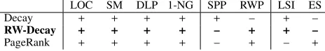
LOC SM DLP 1-NG SPP RWP LSI ES
Decay + + + + + – + –
RW-Decay + + + + – + + –
PageRank + + + + – + – +
Table 1: Summary of our axiomatic characterizations. The plus sign (+) indicates that the centrality measure satisfies the axiom, whereas the minus sign (-) indicates that the cen-trality measure violates it.
tov; hence, from SSP we getFv(G, β)=Fv(G− {(u,w)}, β).
Analogously, ifvhas any outgoing edge, (v,w), then from SSP deleting it does not affect the centrality ofvand we get:
Fv(G, β)=Fv(G− {(v,w)}, β).
It remains to consider a connected graph in which (1) ev-ery node has at most one outgoing edge; (2)vis a sink. Since
Gis connected,vmust have at least one incoming edge. We consider two cases separately:
• Ifvhas exactly one incoming edge, (u,v), then from LOC, DLP and the fact thatuis a sink in graphG− {(u,v)}we get thatFv(G, β)=a·Fu(G− {(u,v)}, β)+β(v).
• Ifvhas at leastk≥2 incoming edges, then—since every node has at most one outgoing edge—these edges must be incident tokdifferent nodes. In such a case, graphGcan be decomposed intokgraphs, (G1, β1), . . . ,(Gk, βk), that
overlap only on nodev, each with exactly one incoming edge tov. These graphs have fewer edges thanG, and in all these graphs,vis a sink. Thus, using SM we get that
Fv(G, β)=Fv(G1, β1)+· · ·+Fv(Gk, βk).
This concludes the proof of Theorem 3.
Finally, let us introduce our last axiom, calledEdge Swap. This axiom states that if two nodes,u,v, have the same cen-trality and the same number of outgoing edges, then their edges are interchangeable. More specifically, if we replace edges (u,u0) and (v,v0) with edges (u,v0) and (v,u0), then the centralities of all nodes will not change. As we will discuss in the next section, this axiom forbids the centrality from promoting the diversity of incoming edges.
Edge Swap (ES):For every graph G node weightβand nodes u,v ∈ V(G)such that Fu(G, β) = Fv(G, β)and
|Γ+G(u)|=|ΓG+(v)|, if(u,u0),(v,v0) ∈E(G), then the fol-lowing holds for every w∈V(G):
Fw(G− {(u,u0),(v,v0)}+{(u,v0),(v,u0)}, β)=Fw(G, β).
The following theorem states that replacing Lack of Self-Impact with Edge Swap in the axiomatization of the Ran-dom Walk Decay centrality results in an axiomatization of PageRank.
Theorem 4. PageRank is the unique centrality measure that satisfies LOC, SM, DLP, 1-NG, ES and RWP.
Proof (Sketch). We use induction on the number of cycles inG. If there are no cycles inG, then the random walk vis-its each node once. Hence, from RWP, the centrality of any node,v, is the same as in the graph without outgoing edges ofvand the thesis follows fromClaim 3from the proof of
Theorem 2 and the fact that for every sink the Random Walk Decay centrality and PageRank are equal.
Now, consider an arbitrary graphGwithkcycles and node weights β. Fix v ∈ V(G) that belongs to some cycle. Let us construct a new graphG0=({v0,w},{(v0,w), . . . ,(v0,w)}), disjoint withG, whereβ(v0)=Fv(G) and|E(G0)|=|Γ+G(v)|.
From LOC we know thatFu(G)=Fu(G+G0) for everyu∈
V(G). Moreover, it can be shown from 1-NG, LOC and SM thatFv0(G0)=β(v0)=Fv(G). Thus, nodesvandv0have the same centralities inG+G0and the same number of outgoing edges. Now, from ES replacing all outgoing edges ofvwith all outgoing edges ofv0does not affect the centralities in the graph. Observe that this operation breaks the cycles thatv
belongs to inG. Hence, the obtained graph has less cycles thanGand the thesis follows from the inductive assumption.
Table 1 summarizes our axiomatic results. Since SPP im-plies LSI, based on Theorem 3 we know that there exists no centrality that satisfies LOC, SM, DLP, 1-NG, SPP and ES.
Comparison with PageRank
Our axiomatic characterizations highlight two differences between the Random Walk Decay centrality and PageRank. In this section, we focus on these two differences and show how they affect the behaviour of these centrality measures.
Strategy-proofness (with respect to outgoing edges)
In many settings, outgoing edges are subject to the node’s decision or manipulations. Examples include the Twitter so-cial network (where outgoing edges represent the accounts that are followed by a user) and the World Wide Web (where outgoing edges represent the links to other websites). Con-sequently, Lack of Self-Impact can be considered a property of strategy-proofness for centrality measures—if outgoing edges do not affect the centrality of a node, then the node has no incentive to manipulate its outgoing connections.
Interestingly, PageRank does not satisfy Lack of Self-Impact. In the following example we show how, by adding outgoing edges, a node can increase its centrality and posi-tion in the ranking according to PageRank, but not according to the Random Walk Decay centrality.
Example 4. Consider graph G from Figure 2. Graph G consists of two 4-cycles,(u1,u2,u3,u4,u1),(v1,v2,v3,v4,v1).
The two cycles are connected via 3 edges:(v4,u4),(u3,v3),
and (u2,v2). Due to the edges connecting both cycles, the
nodes v2, v3, and v4are visited more often (and earlier) by
the random walk, and are thus ranked first by both PageRank and the Random Walk Decay centrality. Node u1, that will be
of our interest, is ranked5th according to both measures. Figure 2 also depicts G0, which is obtained from G by adding the edge(u1,u4). Since this is an outgoing edge for
u1, adding it does not affect the Random Walk Decay
cen-trality of u1. In contrast, this edge has a significant impact
on PageRank of u1. The reason lies in the fact that the
ran-dom walk will now visit u1much more often—whenever the
random walk reaches node u1, with probability1/2it will go
u2
u3
u4
u1
G
v2
v1
v4
v3
u2
u3
u4
u1
v2
v1
v4
v3
G0
Figure 2: Two graphs considered in Example 4, namelyG=
(V,E) andG0=(V,E0) with unit weights:β(v)=1 for every
v∈V. GraphG0is obtained from graphGby adding (u1,u4).
result, both u1 and u4top the ranking according to
PageR-ank. The centralities of all nodes for a=0.8are as follows:
node v PRv(G, β) PRv(G0, β) RW Dv(G, β) RW Dv(G0, β)
v3 6.82(1st) 6.08(3rd) 4.67(1st) 4.36(1st)
v4 6.45(2nd) 5.86(4th) 4.43(2nd) 4.21(2nd)
v2 5.80(3rd) 5.13(5th) 4.13(3rd) 3.77(4th)
u2 4.84(4th) 3.62 3.75(4th) 3.02
u1 4.81(5t h) 6.56(2nd) 3.72(5t h) 3.72(5t h)
u4 4.76 6.95(1st) 3.68 3.94(3rd)
v1 3.58 3.35 2.76 2.60
u3 2.94 2.45 2.48 2.17
In Example 4, a node improved its PageRank by adding an edge to its direct predecessor. In the next section, we will discuss how incoming edges affect both centrality measures.
Diversity (of incoming edges)
One of the characteristic properties of PageRank is its recur-sive formula (see (2)), which states that PageRank of a node depends solely on PageRank of its direct predecessors (or, more precisely, nodes incident to its incoming edges). Intu-itively speaking, PageRank of a node does not depend on the position in the network of its predecessors, but only on their centrality. In our axiomatic characterization, this prop-erty is captured by Edge Swap, which implies that an incom-ing edge from a node with the lowest centrality in a densely connected part of the graph could be as profitable as an in-coming edge from a node with the highest centrality in a different, less densely connected part.
The Random Walk Decay centrality does not satisfy Edge Swap. In fact, the node can achieve higher centrality if it has incoming edges from a diverse set of nodes, i.e., com-ing from different parts of the network. We demonstrate this point with the following example.
Example 5. Consider graph G from Figure 3. This graph consists of three more densely connected parts, so called
communities: {u1,u2,u3}, {v1,v2,v3} and {w1,w2,w3,w4}.
These communities are connected through nodes u1,v1,w1
which form a 3-clique. Since w1 belongs to the biggest
community, both its Random Walk Decay centrality and its PageRank are the highest. The nodes u1and v1have the
sec-ond highest values, with symmetrical positions in the graph. Figure 3 also depicts the graph G0, which is obtained from
G by rewiring the two highlighted (red) edges. Specifically, the edges(u2,u1)and (v2,v1)are replaced by (u2,v1)and
u3
u2
u1 w1
w2 w4
w3
v1 v3
v2
G
u3
u2
u1 w1
w2 w4
w3
v1 v3
v2
G0
Figure 3: Two graphs considered in Example 5, namely
G=(V,E) andG0=(V,E0) with unit weights:β(v)=1 for everyv∈V. GraphG0is obtained from graphGby replacing edges (u2,u1) and (v2,v1) with edges (u2,v1) and (v2,u1).
(v2,u1); in result, the two new edges connect two
commu-nities. Since u2and v2both have two edges and clearly the
same centralities in graph G, from Edge Swap we know that PageRank of every node in G0is the same as in G. In
con-trast, the centralities of both nodes u1 and v1 increase
ac-cording to the Random Walk Decay centrality. This is be-cause, according to this centrality, an edge from a different community is more profitable than an edge from your own community. In our example, the random walk that starts from nodes v2and v3reaches node u1faster in graph G0; the same
holds for node v1. In result, in G0, the Random Walk Decay
centralities of u1 and v1 are higher than the Random Walk
Decay centrality of node w1. The centralities of all nodes for
a=0.8are:
node v PRv(G, β) PRv(G0, β) RW Dv(G, β) RW Dv(G0, β)
w1 7.15(1st) 7.15(1st) 4.40(1st) 4.40(3rd)
u1 7.06(2nd) 7.06(2nd) 4.15(2nd) 4.46(1st)
v1 7.06(2nd) 7.06(2nd) 4.15(2nd) 4.46(1st)
w3 4.33(4th) 4.33(4th) 2.62 2.62
w2,w4 4.16(5th) 4.16(5th) 2.74(4th) 2.74
u2,v2 4.02 4.02 2.56 2.85(4th)
u3,v3 4.02 4.02 2.56 2.70
Example 5 shows that the Random Walk Decay cen-trality increases when incoming edges become more di-verse. As such, it avoids putting at the top of the rank-ing several nodes from the same community, which of-ten happens in PageRank (Avrachenkov and Litvak 2006; Zhirov, Zhirov, and Shepelyansky 2010).
Related Work
Our paper belongs to a line of papers that study the ax-iomatic properties of centrality measures (Boldi and Vigna 2014; Bloch, Jackson, and Tebaldi 2016; Skibski, Michalak, and Rahwan 2018). In particular, our axiomatization of the Decay centrality relies on a recent axiomatization for undi-rected graphs proposed by Skibski and Sosnowska (2018).
PageRank in its general form. Our new axiomatization sig-nificantly differs from all of these axiomatizations.
Conclusions
In this paper, we proposed Random Walk Decay centrality— a new centrality measure based on the random walk. We pro-vided an axiomatic characterization using six axioms, and proved that replacing only one property leads to an axiomati-zation of the Decay centrality. Furthermore, we showed that Random Walk Decay works similarly to PageRank, but has certain properties that can be more desirable in various set-tings. In our future work, we plan to perform a comparative experimental analysis of Random Walk Decay and PageR-ank using real-world networks.
Acknowledgements
This work was supported by the Foundation for Polish Sci-ence within the Homing programme (Project title: “Central-ity Measures: from Theory to Applications”) and the Polish National Science Center grant 2016/23/B/ST6/03599.
References
Altman, A., and Tennenholtz, M. 2005. Ranking systems: the PageRank axioms. InProceedings of the 6th ACM Con-ference on Electronic Commerce (ACM-EC), 1–8.
Avrachenkov, K., and Litvak, N. 2006. The effect of new links on google pagerank. Stochastic Models 22(2):319– 331.
Bianchini, M.; Gori, M.; and Scarselli, F. 2005. Inside pagerank.ACM Transactions on Internet Technology (TOIT)
5(1):92–128.
Bianzino, A. P.; Chaudet, C.; Rossi, D.; Rougier, J.-L.; and Moretti, S. 2011. The green-game: Striking a balance be-tween qos and energy saving. InTeletraffic Congress (ITC), 2011 23rd International, 262–269.
Bloch, F.; Jackson, M. O.; and Tebaldi, P. 2016. Centrality measures in networks.Available at SSRN 2749124. Boldi, P., and Vigna, S. 2014. Axioms for centrality.Internet Mathematics10(3-4):222–262.
Borgatti, S. P. 2005. Centrality and network flow. Social networks27(1):55–71.
Freeman, L. C. 1979. Centrality in social networks: Con-ceptual clarification.Social Networks1(3):215–239.
Freeman, L. C. 2008. Going the wrong way on a one-way street: Centrality in physics and biology. Journal of Social Structure9(2):1–15.
Hinz, O.; Skiera, B.; Barrot, C.; and Becker, J. U. 2011. Seeding strategies for viral marketing: An empirical com-parison.Journal of Marketing75(6):55–71.
Huberman, B. A.; Pirolli, P. L.; Pitkow, J. E.; and Lukose, R. M. 1998. Strong regularities in world wide web surfing.
Science280(5360):95–97.
Jackson, M. O. 2008. Social and economic networks, vol-ume 3. Princeton university press.
Koschützki, D.; Lehmann, K. A.; Tenfelde-Podehl, D.; and Zlotowski, O. 2005. Advanced centrality concepts. In Net-work Analysis, volume 3418 ofLecture Notes in Computer Science. Springer. 83–111.
Lerman, K., and Ghosh, R. 2010. Information contagion: An empirical study of the spread of news on digg and twitter social networks. Icwsm10:90–97.
Lovász, L. 1993. Random walks on graphs: A survey. Com-binatorics, Paul Erdos is eighty2(1):1–46.
Newman, M. E. 2005. A measure of betweenness centrality based on random walks. Social networks27(1):39–54. Newman, M. 2010. Networks: an introduction. Oxford university press.
Page, L.; Brin, S.; Motwani, R.; and Winograd, T. 1999. The PageRank citation ranking: bringing order to the web.
Stanford InfoLab.
Palacios-Huerta, I., and Volij, O. 2004. The measurement of intellectual influence.Econometrica72(3):963–977. Palbom, A. 2005. Complexity of the directed spanning cac-tus problem.Discrete applied mathematics146(1):81–91. Sabidussi, G. 1966. The centrality index of a graph. Psy-chometrika31(4):581–603.
Skibski, O., and Sosnowska, J. 2018. Axioms for distance-based centralities. InProceedings of the 32nd AAAI Confer-ence on Artificial IntelligConfer-ence (AAAI), 1218–1225.
Skibski, O.; Rahwan, T.; Michalak, T. P.; and Yokoo, M. 2016. Attachment centrality: An axiomatic approach to con-nectivity in networks. InProceedings of the 15th Interna-tional Conference on Autonomous Agents and Multiagent Systems (AAMAS), 168–176.
Skibski, O.; Michalak, T. P.; and Rahwan, T. 2018. Ax-iomatic characterization of game-theoretic centrality. Jour-nal of Artificial Intelligence Research62:33–68.
White, S., and Smyth, P. 2003. Algorithms for estimat-ing relative importance in networks. InProceedings of the 9th ACM SIGKDD International Conference on Knowledge Discovery and Data Mining, 266–275. ACM.
W ˛as, T., and Skibski, O. 2018. Axiomatization of the PageRank centrality. In Proceedings of the 27th Interna-tional Joint Conference on Artificial Intelligence (IJCAI), 3898–3904.