Middlesex University Research Repository
An open access repository of
Middlesex University research
http://eprints.mdx.ac.uk
Kim, Thai Young ORCID: https://orcid.org/0000-0003-4504-689X, Dekker, Rommert and Heij, Christiaan (2017) Spare part demand forecasting for consumer goods using installed base
information. Computers and Industrial Engineering, 103 . pp. 201-215. ISSN 0360-8352 (doi:10.1016/j.cie.2016.11.014)
Final accepted version (with author’s formatting)
This version is available at:http://eprints.mdx.ac.uk/28101/
Copyright:
Middlesex University Research Repository makes the University’s research available electronically.
Copyright and moral rights to this work are retained by the author and/or other copyright owners unless otherwise stated. The work is supplied on the understanding that any use for commercial gain is strictly forbidden. A copy may be downloaded for personal, non-commercial, research or study without prior permission and without charge.
Works, including theses and research projects, may not be reproduced in any format or medium, or extensive quotations taken from them, or their content changed in any way, without first obtaining permission in writing from the copyright holder(s). They may not be sold or exploited commercially in any format or medium without the prior written permission of the copyright holder(s).
Full bibliographic details must be given when referring to, or quoting from full items including the author’s name, the title of the work, publication details where relevant (place, publisher, date), pag-ination, and for theses or dissertations the awarding institution, the degree type awarded, and the date of the award.
If you believe that any material held in the repository infringes copyright law, please contact the Repository Team at Middlesex University via the following email address:
The item will be removed from the repository while any claim is being investigated.
1
Spare part demand forecasting for consumer goods
using installed base information
Abstract
When stopping production, the manufacturer has to decide on the lot size in the final production run to cover spare part demand during the end-of-life phase. This decision can be supported by forecasting how much demand is expected in the future. Forecasts can be obtained from the installed base of the product, that is, the number of products still in use. This type of information is relatively easily available in case of B2B maintenance contracts, but it is more complicated in B2C spare parts supply management. Consumer decisions on whether or not to repair a malfunctioning product depend on the specific product and spare part. Further, consumers may differ in their decisions, for example, for products with fast innovations and changing social trends. Consumer behavior can be accounted for by using appropriate types of installed base, for example, lifetime installed base for essential spare parts of expensive products with long lifecycle, and warranty installed base for products with short lifecycle. This paper proposes a set of installed base concepts with associated simple empirical forecasting methodologies that can be applied in practice for B2C spare parts supply management during the end-of-life phase of consumer products. The methodology is illustrated by case studies for eighteen spare parts of six products from a consumer electronics company. The research hypotheses on which installed base type performs best under which conditions are supported in the majority of cases, and forecasts obtained from installed base are substantially better than simple black box forecasts. Incorporating past sales via installed base therefore supports final production decisions to cover future consumer demand for spare parts.
Keywords
2 1 Introduction
For owners and users, it is frustrating if a product or system can no longer be used because a small component failed and spare parts are not available. The timely availability of spare parts is therefore an important issue for users, especially for ageing products. Providing spare parts, however, is a challenge for Original Equipment Manufacturers (OEMs), as users can be spread over the world and demand is typically intermittent (Boylan and Syntetos, 2009). In many cases, demand is high for some parts and very small for other parts, resulting in surplus stocks. Forecasting the location and size of demand per spare part is therefore an important aspect in spare parts management. It plays a major role in determining the final production run that should guarantee parts availability for the remaining service life (see e.g. Van der Heijden and Iskandar, 2013). It is also important to determine where and how much parts should be in stock, especially if the demand is decreasing.
Much research has been devoted to forecasting spare parts demand. Boylan and Syntetos (2009) give a recent overview of methods available so far. They propose a three phase approach, with pre-processing, processing and post-processing. In the pre-processing phase, one classifies the spare parts and selects the forecasting method, which is then applied per class in the second phase. Finally, the obtained forecasts are adjusted in the post-processing phase. The forecasting methods considered by Boylan and Syntetos (2009) are all based on demand data only, without taking any other information into account, similar to forecasting sales of new products. However, forecasting spare parts demand differs from forecasting demand for new products because spare parts are only needed to repair products which are still in use. Hence the location and number of products in use, also called the Installed Base (IB), is of primary interest as generator of spare parts demand. Several authors, including Jalil et al. (2011) and Dekker et al. (2013), have therefore proposed to use IB as the causal variable in forecasting spare parts demand. This kind of approach requires that companies keep track of their IB. That is possible in B2B cases, such as planes (Fokker Services), high-end computers (IBM), or advanced chip making machines (ASML), as users of these expensive systems have service contracts with manufacturers to guarantee timely parts supply. IB forecasting then consists of establishing the demand per product and forecasting the future development of IB. This two-step forecasting procedure does require some work in practice because products may have been adapted for customers and demand may also be influenced by local conditions (Jalil et al., 2011).
3
demand of spare parts. In this paper, we therefore introduce new part classifications and related installed base concepts that can be used in the pre-processing phase of forecasting consumer demand for spare parts and that require a relatively limited amount of management information. The proposed installed base concepts are lifetime IB, warranty IB, economic IB, and mixed IB. Use of lifetime IB assumes that all products stay in the market according to their expected lifetime, which holds mostly for expensive products. Warranty IB assumes that spare parts demand is limited to products for which a warranty still applies. Economic IB assumes that products are discarded when repairs are no longer economic, which is relevant especially for products that evolve quickly, for example, due to technological innovations. Finally, mixed IB is a refinement of economic IB that applies when consumers show heterogeneity in their evaluation of the costs and benefits of repair. These IB concepts will be elaborated and they will be empirically validated through a comparison with standard forecasting for a sample of real cases drawn from a major consumer products manufacturer.
The remainder of this paper is structured as follows. Section 2 discusses some background literature, presents the employed concepts of installed base, and formulates the main research hypotheses. The methodology is described in Section 3, and it is illustrated in detail for a specific spare part in Section 4. Section 5 presents the results for a set of eighteen spare parts related to six products. Section 6 concludes and summarizes operational implications.
2 Installed base
2.1 Background literature
The main topic of this paper is spare part demand forecasting for consumer products over their end-of-life phase, using the concept of installed base (IB). We review some background literature on IB forecasting and on the end-of-life production decision, where it should be noted that the term ‘installed base’ has not always been used in the past for describing this concept.
4
with data from an automobile factory. Jin and Liao (2009) use IB within a simulation context for inventory control to satisfy maintenance demand for spare parts and assume that the IB is known. Thereafter, Jalil et al. (2010) describe further experience with IBM and highlight the value of the IB concept. Dekker et al. (2013) review the use of this concept and its application at several companies. Minner (2011) combines reliability models with inventory control to arrive at better forecasts than those obtained by time series analysis, and he evaluates his approach by simulation data. Jin and Tian(2012) use the IB concept in optimizing inventory control policies in case of increasing demand. They illustrate their method by simulations and they do not consider forecasting. Bacchetti and Saccani (2012) provide an extensive overview of spare parts demand forecasting. They investigate the currently still existing gap between research and practice in spare parts management, and they also identify issues in obtaining the IB, using information from Wagner and Lindemann (2008). Finally, Chou et al. (2015) use the concept of IB to forecast final orders of automobile parts. Their first finding is that production costs are higher during EOL than during the mature phase because of loss of economies of scale and of economies of scope. Second, they find that the optimal warranty period during EOL depends on product failure rates.
5
at the start of the EOL phase is similar to ours, but they consider only simulated data and no real-world spare part demand data.
2.2Installed base concepts
Traditionally, demand forecasting is based on simple extrapolation of historical data. Such so-called black-box methods are popular because of their simplicity, as the required information is limited to historical demand data. For time series of (weekly, monthly, quarterly, or yearly) data, these methods have become widespread in business since the work of Box and Jenkins(1976). For spare parts demand, the past sales of products that contain the part are evidently also relevant. The installed base of the product is the number of sold products that is in use and can therefore lead to demand of its spare parts. More precisely, we define the lifetime installed base as follows. For each time period (week, month, quarter, or year), the lifetime installed base increases with the quantity that leaves the warehouse and it declines with the number of returned products and with the number of products exceeding the expected lifetime. This definition is similar to what Wagner and Lindemann (2008) propose for spare parts business of engineering companies. Consumer (electronic) products are typically sold through independent retailers who do not share sales information with manufacturers. For the electronics company in our case study, it generally takes between two and three weeks after leaving the warehouse before the products are sold and enter the customer base. The sales and demand data are typically available on a weekly basis. Let S(t) be the product sales to customers in week t, let R(t) be the returns from customers of that week, and let L denote the average lifetime of the product, including second-hand usage. Then lifetime installed base (IBL) at the end of week t is defined as follows
IBL(t) = ∑𝑡𝑡 (𝑆𝑆(𝑖𝑖)− 𝑅𝑅(𝑖𝑖))
𝑖𝑖=𝑡𝑡−𝐿𝐿+1
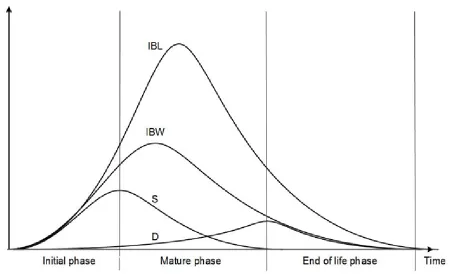
(where sales start in period 1 and S(i) and R(i) are defined as 0 for times i < 1). Inderfurth and Mukherjee (2008) discuss the typical shape of IBL, as shown in Figure 1. This shape is characterized by three phases in the product life cycle. First is the initial phase with growing sales per time unit, followed by a mature phase where sales gradually fall back. The IBL curve in Figure 1 therefore has an inflection point where the initial phase passes into the mature phase. Finally comes the end-of-life phase, where the product is no longer produced. Demand for spare parts may be expected to be relatively low in the initial phase, as most products are relatively young and will generally function well. This demand is expected to rise during the mature phase and possibly also during early parts of the EOL phase, whereas later on, demand will gradually diminish as more products reach their lifetime.
<< Insert Figure 1 about here. >>
6
over-estimate actual demand, because the increasing demand trends during the mature phase will eventually break down somewhere during the EOL phase, because customers discard the products. Pince and Dekker (2011) report similar problems for forecasts based on exponential smoothing.
Figure 1 shows also the typical shape of what we call the warranty installed base. Consumers may determine their demand decision for repair based on product warranty regulations. The warranty period is the maximum duration for which the company supports sustainability of the product at its own expense. After this period, customers have to carry costs of repair and logistics by themselves, which may lead them to purchase a new product instead of asking repair of the old one. For a warranty period of W periods, the warranty installed base (IBW) is
IBW(t) = ∑𝑡𝑡 (𝑆𝑆(𝑖𝑖)− 𝑅𝑅(𝑖𝑖))
𝑖𝑖=𝑡𝑡−𝑊𝑊+1 .
(again with S(i) = R(i) = 0 for i < 1). As the warranty period is smaller than the average lifetime of most consumer products, IBW is identical to IBL during the first W sales periods and IBW becomes smaller than IBL afterwards.
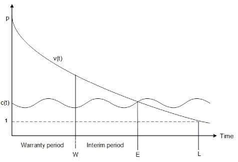
After expiration of the warranty period, consumers may still generate demand for spare parts. Such behavior is rational if the remaining economic value of the product after repair exceeds the repair costs. This leads us to the concept of economic installed base (IBE), of which the defining ingredients are shown in Figure 2. We use the following notation. For period t, let c(t) be the repair costs, let vi(t) be the remaining economic value of the product bought in week i, and let
the economic decision for repair be denoted by Ei(t) = 1 if vi(t) > c(t) and Ei(t) = 0 if vi(t) ≤ c(t).
Then the economic installed base is defined as that part of the lifetime installed base for which repair is economical, that is,
IBE(t) = ∑𝑡𝑡𝑖𝑖=𝑡𝑡−𝐿𝐿+1𝐸𝐸𝑖𝑖(𝑡𝑡) × (𝑆𝑆(𝑖𝑖)− 𝑅𝑅(𝑖𝑖)).
(with S(i) = R(i) = 0 for i < 1). To make this base operational, values of repair costs and remaining value are needed. In our case study, we will take the price of the spare part as the repair cost. We do not incorporate handling and labor costs, as these cost figures are not available and vary per customer location and per type of failure. This choice implies under-estimation of actual costs, and hence over-estimation of the actual economic installed base. In other applications, more accurate values of IBE can be obtained if more accurate cost information is available. The remaining value vi(t) is determined by assuming exponential value decay and final unity value at the end of average
lifetime. Let pi (>1) be the price of the product sold in period i, then the decay rate ai for products
sold in that period is obtained from the condition that 1 = pi×exp(ai×L), so that ai = -ln(pi)/L. The
remaining value in period t is equal to vi(t) = pi×exp(ai×(t-i)).
7
2 sketches the remaining value v(t) of a product bought at time t = 0 for price p, where it remains economically attractive to pay the repair cost c(t) until time E. Our concept of economic installed base is based on a trade-off between value and costs made by consumers after expiration of the warranty period and somewhat resembles the trade-off between repair and replacement costs made by manufacturers during the warranty period as studied by Pourakbar et al. (2012).
<< Insert Figure 2 about here. >>
In the construction of IBE, it is assumed that all consumers apply the same decay rate for remaining value of the product. Consumers may differ in their subjective evaluation of remaining value, for example, if they vary in their sensitivity for social trends and technological innovations. The decision on whether or not it is economical to repair the product will then depend on heterogeneous tastes. For this situation of mixed economic decisions, we define the mixed economic installed base (IBM) similar to IBE, but with varying perceived lifetimes so that value decay rates are heterogeneous across users. In our IBM applications, we follow Rogers (2003) and divide consumers in five adopter segments. Early adopters replace the product relatively fast, corresponding to a relatively short lifecycle. In line with Rogers (2003), the consumers are distributed as follows over the segments (in parenthesis is the lifecycle within each segment, as fraction of the overall average): 2.5% innovators (0.6), 13.5% early adopters (0.7), 34% early majority (1.0), 34% late majority (1.05), and 16% laggards (1.3).
2.3Research hypotheses
As discussed in the literature review, the distinguishing feature of our research on installed base is that we consider its use in forecasting real-world demand for spare parts of consumer products during the end-of-life phase. Previous studies concerned either demand for end products instead of spare parts, or demand for spare parts arising from maintenance contracts with large clients and with operational information on the number of products in use, or simulation studies instead of real demand data. The main question in forecasting consumer spare part demand with installed base is which type of base gives the best information. The answer to this question is likely to depend on characteristics of the spare part and of the product. We formulate a set of research hypotheses, which are tested empirically in Sections 4 and 5.
8
costs. Obviously, the benefits are larger for longer life times. The third hypothesis is that economic installed base works best for non-essential spare parts of products with long lifetime. This situation corresponds to a relatively long interim period in Figure 2, where users can decide to repair non-essential parts if the remaining lifetime is long enough to compensate repair costs. If repair of the spare part is relatively expensive but not mandatory, then the product can simply still be used without repair. Finally, the fourth hypothesis is that mixed economic installed base works best if consumers differ much in their acceptance of new products. If, for example, many consumers switch to a new product before the old one has lost its function, then spare part demand for the old product falls below what is expected from a purely economic point of view. This kind of behavior can be observed in particular for innovative products if consumers derive higher utility from switching to a new product than from prolonged use of the old product. Pourakbar et al (2012) mention the example of cathode ray tubes (CRT) for TV’s and monitors, where CRT failures often lead users to switch to liquid crystal display (LCD), plasma, or organic light emitting diode (OLED) screens even if CRT repair would still be economically profitable when measured by expected gained lifetime.
3 Forecast methodology
3.1 Installed base and spare part demand
As we wish to use installed base to predict real-life spare part demand for consumer products, we need a model that relates installed base to this demand in terms of the available empirical information. In order to set up our model, we first make a set of simplifying assumptions that will later be relaxed. We first assume that the product is sold only in period 0 and that the spare part is so cheap that it will be replaced when it breaks down. As time goes by, ageing of the product affects spare part demand in two ways, that is, wear-out and end-of-use. For a given customer, let T1 be the (continuously measured) time of failure of the product requiring a spare part for repair,
and let T2 be the (continuously measured) time where this customer ends use of the product. Both
times can be seen as random variables, with survival distributions Si(t) = Pi(Ti > t), i = 1,2. This
customer will not demand the spare part if T1≥ T2. The demand probability pd(t) in period t, that
runs in continuous time from t-1 to t, is equal to the joint probability P(t-1 < T1 < t, T2 > t). Assume
that the probability of break-down does not depend on the decision of continued product use, that is, P(t-1 < T1 < t | T2 > t) = P(t-1 < T1 < t), then the demand probability is
pd(t) = P(t-1 < T1 < t, T2 > t) = P(t-1 < T1 < t) × P(T2 > t) = (S1(t-1) – S1(t))×S2(t). (1)
9
pd(t) = (exp(-a1(t-1)) – exp(-a1t))×exp(-a2t) = (exp(a1) – 1)×exp(-(a1 + a2)t). (2)
This is the probability per customer of demand in period t. The expected total demand D(t) in period t, with remaining installed base IB(t), is equal to pd(t)×IB(t). Let b0 = ln(exp(a1) – 1) and b2
= -(a1 + a2), then (2) gives
ln(D(t)) = b0 + ln(IB(t)) + b2×t. (3)
This relation has been obtained under various simplifying assumptions. The variable t in (3) denotes the age of the product, which depends on the moment it was bought. If we neglect product disuse, as this information is usually not available to the manufacturer, then installed base in period t is IB(t) = ∑𝑡𝑡 𝑋𝑋(𝑡𝑡 − 𝑠𝑠)
𝑠𝑠=1 , where X(t – s) are the sales in the period s time units before the current
one. Then expected demand in period t is 𝐷𝐷(𝑡𝑡) =∑𝑡𝑡 𝑝𝑝𝑑𝑑(𝑠𝑠)𝑋𝑋(𝑡𝑡 − 𝑠𝑠) =
𝑠𝑠=1 𝑒𝑒𝑏𝑏0∑𝑡𝑡𝑠𝑠=1𝑒𝑒𝑏𝑏2𝑠𝑠𝑋𝑋(𝑡𝑡 − 𝑠𝑠).
The past sales information captured by installed base is not rich enough to retrieve this expected demand, as it only stores the sum-total of past sales and not the specific distribution of sales over the various periods. An approximation of expected demand is obtained by replacing the age-specific weights (𝑒𝑒𝑏𝑏2𝑠𝑠) by a single weighting factor evaluated at the weighted age of the products,
that is, 𝑒𝑒𝑏𝑏2AGE(t) where AGE(t) is the mean age of the installed base in period t. This approximation
gives D(t) = 𝑒𝑒𝑏𝑏0𝑒𝑒𝑏𝑏2AGE(t)∑𝑠𝑠=1𝑡𝑡 𝑋𝑋(𝑡𝑡 − 𝑠𝑠) = 𝑒𝑒𝑏𝑏0𝑒𝑒𝑏𝑏2AGE(t) IB(t), or
ln(D(t)) = b0 + ln(IB(t)) + b2× AGE(t). (4)
The coefficient 1 of logarithmic installed base follows from the assumptions that no products are disused and that every break-down of the product results in demand for repair. We replace this coefficient by an arbitrary one to account for the fact that some products will be disused and only a portion of all break-downs will be repaired, as the owner can also decide to buy a new product. The resulting relation is
ln(D(t)) = b0 + b1×ln(IB(t)) + b2×AGE(t). (5)
10 3.2Estimation and model selection
Our modelling approach is rather pragmatic. The amount of relevant available demand data is generally limited, so we do not assume to know all details of the data generating process. For example, we do not know the purchase dates of products that lead to spare part demand. Our ambition is therefore limited to produce reasonably accurate forecasts and we choose for rather simple models that are evaluated in terms of their out-of-sample forecast performance. For our case study, we present forecast results that are all based on model (5). We also considered richer specifications, for example, including squared age, but the data available for estimation were in general not rich enough to improve forecasting power. Model (5) corresponds to a regression model if we add an unobserved error ε(t) term to account for the (unknown) approximation errors of actual demand behavior. Further, to allow for zero values of demand and installed base, the estimated model is specified as follows.
ln(1+D(t)) = b0 + b1×ln(1+IB(t)) + b2×AGE(t) + ε(t). (6)
For simplicity, the error term is assumed to follow an autoregressive (AR) process, because the unknown coefficients b0, b1, and b2 in (6) can then be estimated simply by ordinary least squares.
We could allow for more general error correlation structures like ARMA, but this would complicate the estimation and forecasting tasks and could easily cause over-fitting because of the relatively short time interval that is available for estimation in most practical applications. As the actual weekly demand data of the case study spare parts are quite erratic, these demand data are smoothed by taking an exponentially weighted moving average (EWMA), and we have chosen for smoothing factor 0.06. We did not try to optimize the EWMA smoothing factor in order to prevent over-fitting and we simply used the value of 0.06 that has become popular since RiskMetrics of J. P. Morgan(1996). This means that the demand of the current week gets weight 0.06, whereas the combined weight of previous weeks is 0.94. We compared the results for this choice of left-hand variable in (6) with two other options: without weighting, that is, using actual weekly demand, or with eight-week averaging, as the company needs an average lead time of eight weeks to cover unanticipated demand. We found that models estimated from EWMA smoothed demand, denoted by Ds(t), work best in forecasting, not only to forecast EWMA demand, but also to forecast actual
demand and its eight-week average.
Black box forecasts are obtained from pure AR models, that is, with b1 = b2 = 0 in (6), and
with b0 estimated from the demand data of the initial and mature product phases. The error term is
modeled as ε(t) = c1×ε(t-1) + … + cp×ε(t-p) + ω(t), where ω(t) is a white noise process and where
11
will only consider pure AR models.
The AR order of the black box model is also used in all installed base models. The corresponding model (6) is estimated for the initial and mature phase of the product for each of the four considered installed base types, that is, IBL, IBW, IBE, and IBM. The mean age is defined in terms of the corresponding installed base type, for example, using only products under warranty in the model with IBW. The installed base term ln(1+IB(t)) is removed from the model if it has a negative coefficient (b1 < 0), as it is a natural requirement that demand is positively related to
installed base (for given mean age). Although the above analysis for fixed hazard rates suggests that the coefficient of the mean age term AGE(t) should be negative (b2 < 0), we do not impose
this condition. The reason is that other hazard rates provide other age effects, and it is not illogical that spare part demand could increase for higher mean age of the installed base. Insignificant terms are not removed from the model, because insignificance may be due to a short estimation period for the model.
We summarize the steps needed to estimate the candidate models for spare part demand during the initial and mature product phases. First, determine the following characteristics of the product: average lifetime, sales for each period during the initial and mature phases. From the sales data, determine the numerical values of installed base types IBL, IBW, IBE, and IBM, for each period over the full life cycle (initial, mature, and EOL phases). This requires information on warranty period (for IBW), cost of the spare part (for IBE), and consumer segmentation (for IBM). For each installed base, compute the associated values of mean age for each period of the full life cycle. Next, determine the spare part demand data for each period during the initial and mature phases, and compute smoothed values by EWMA. For these smoothed demand data, estimate an AR model and select the AR order p. Estimate four types of installed base models, each with the same AR order, and keep the installed base variable only if it has a positive coefficient.
3.3Forecast evaluation
The procedure described in the previous section provides a set of five models (AR, IBL, IBW, IBE, and IBM) that can be used to forecast spare part demand over the EOL phase. These forecasts use only information that is available at the end of the mature phase, as no EOL information is of course available at the start of EOL. Note, however, that the values of installed base and mean age are completely determined by product sales before EOL, so that these variables can be extrapolated perfectly for the full EOL phase. The forecasts are determined iteratively, as the AR structure implies that forecasts of previous periods affect the forecast for the current period. These forecasts for earlier periods during EOL are not replaced by realized demands, because this information is not available at the start of EOL. The forecasts concern the variable ln(1+Ds(t)), which are easily
translated into forecasts of Ds(t). For periods where the installed base is zero, the forecasted
12
prevent erratic behavior, the model forecasts are not “unsmoothed’, and the forecasts of Ds(t) are
directly compared with actual demand D(t).
The forecast performance of the various models can be compared graphically with actual demand by means of a joint time plot for the EOL phase. The forecasts are also numerically compared by means of the following three criteria. The summed error is the difference between the summed forecasts and the summed demand over the EOL phase. Suppose that actual demand data D(t) are available for periods t1 ≤ t ≤ t2 of the EOL phase, and let F(t) be the forecasts for
these periods; then
SUM = ∑𝑡𝑡2 (𝐹𝐹(𝑡𝑡)− 𝐷𝐷(𝑡𝑡))
𝑡𝑡=𝑡𝑡1 / ∑ 𝐷𝐷(𝑡𝑡)
𝑡𝑡2
𝑡𝑡=𝑡𝑡1 . (7)
Positive values correspond to over-estimation of the total need for spare parts during EOL, and negative values correspond to under-estimation. This is our main criterion to compare forecast methods, as it is measures the global quality of forecasting the spare part need during EOL. We also consider two other criteria that measure the local, week-by-week forecast quality, that is, the mean absolute prediction error (MAPE) and the root mean squared prediction error (RMSPE).
MAPE = ∑𝑡𝑡2𝑡𝑡=𝑡𝑡1|𝐹𝐹(𝑡𝑡)−𝐷𝐷(𝑡𝑡)|
∑𝑡𝑡2𝑡𝑡=𝑡𝑡1𝐷𝐷(𝑡𝑡) , RMSPE =
�𝑡𝑡2−𝑡𝑡1+11 ∑𝑡𝑡2 (𝐹𝐹(𝑡𝑡)−𝐷𝐷(𝑡𝑡))2 𝑡𝑡=𝑡𝑡1
1
𝑡𝑡2−𝑡𝑡1+1∑𝑡𝑡2𝑡𝑡=𝑡𝑡1𝐷𝐷(𝑡𝑡) =
�∑𝑡𝑡2 (𝐹𝐹(𝑡𝑡)−𝐷𝐷(𝑡𝑡))2 𝑡𝑡=𝑡𝑡1
∑𝑡𝑡2𝑡𝑡=𝑡𝑡1𝐷𝐷(𝑡𝑡)/�𝑡𝑡2−𝑡𝑡1+1 . (8)
4 Illustrative case: compressor of refrigerator
4.1Product and demand characteristics
The spare parts in our case study are provided by the Western European warehouse of Samsung Electronics. Refrigerators are one of their products with a relatively stable sales pattern. In this section, we analyze the demand for the compressor of a specific type of refrigerator, which we call type 1 to distinguish it from another refrigerator type 2 that is studied in the next section. The compressor is indispensable, as the refrigerator does not function if the compressor is out of order. Compressors are very reliable, and malfunctioning is mainly caused by extreme operating conditions. The compressor is somewhat expensive, as it costs about 100 euro, which is about 18.3 percent of the price of around 550 euro of the refrigerator. The warranty period is 2 years, and the average lifetime of refrigerators is 13 years according to the National Association of Home Builders (2007), which is relatively long for consumer electronics products.
13
from the formula in Section 2.2 for the (yearly) decay rate, a= -ln(p)/L = -ln(550)/13 = -0.485. The remaining value is 18.3 percent when 0.183 = exp(-0.485×y), that is, after y = 3.5 years. The interim period of Figure 2, starting after the warranty period of 2 years, is therefore only 1.5 years. This is rather short for products with an average replacement cycle of 13 years, so that we do not expect large differences between economic and warranty installed base during initial periods. As refrigerators are such stable products, we expect that many consumers are willing to replace the compressor at their own cost for the benefit of considerable extra lifetime of the refrigerator. Our hypothesis is therefore that IBL will provide the best forecasts, better than black box (AR) and alternative installed base types (IBW, IBE, and IBM).
<< Insert Figure 3 about here. >>
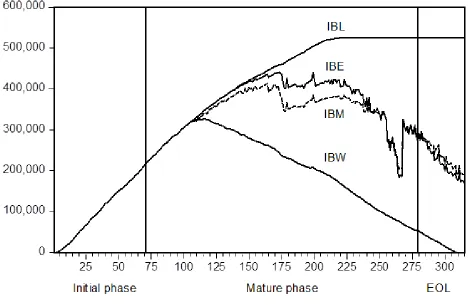
Time plots of the various installed base types are shown in Figure 3. All installed base types are very similar in the initial phase, but start to get differentiated in the mature phase. The sales data run from week 12 in 2008, when sales of this refrigerator started, to week 29 of 2013, when sales ended. Weekly replacement data for the compressor are available from week 12 in 2008 to week 13 of 2014. Total sales of the refrigerator are more than half a million, and the total replacement demand for compressors is 5,678, of which 247 occur in the observed EOL phase. The six years of observations, with 279 weekly sales and 315 weekly demand data, cover less than half of the lifecycle of the product, and the observed EOL phase is only 36 weeks. The forecasting task is to predict demand for these 36 weeks, and there is a relatively long estimation period of 279 weeks for the initial and mature periods. As the case study has been conducted in April 2014, we are not able to evaluate forecasts beyond week 13 of 2014.
<< Insert Figure 4 about here. >>
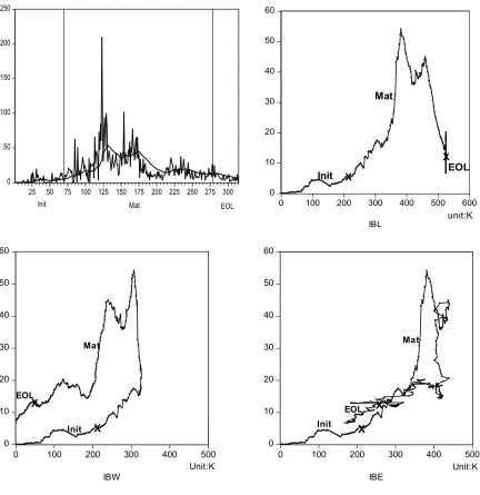
The top left diagram in Figure 4 shows a time plot of weekly demand during 315 weeks, as well as its EWMA smoothed version. The other diagrams show scatter plots, with EWMA smoothed demand on the vertical axis and installed base (IBL, IBW, and IBE) on the horizontal axis. The task is to determine a relation between installed base and demand from data for the initial and mature phases, and to use this relation to forecast demand during EOL. The scatter diagrams indicate that this is not an easy task, as this relation changes among the various phases of the product. If, for example, one would fit a straight line in the IBW scatter diagram for the initial and mature phases, then this would systematically over-estimate actual demand during the EOL phase. It seems very difficult to make a choice among alternative installed base types solely from the statistical data information in the initial and mature phases. In the foregoing, we used economic arguments on consumer behavior to motivate the choice for IBL.
4.2 Forecast results
The obtained black box model is the following AR(2) model: ln(1+Ds(t)) = 3.30 + ε(t), with ε(t) =
14
data, with R2 = 0.997. Each of the four installed base models has a negative coefficient for installed
base, so that this variable is removed. The reduced models contain mean age and AR(2) error terms. The mean age variable has an insignificant negative coefficient in all cases, with the following (one-sided) p-values: 0.09 for IBL, 0.44 for IBW, 0.47 for IBE, and 0.40 for IBM. Even though the effects are weak, we try to exploit this installed base information in forecasting.
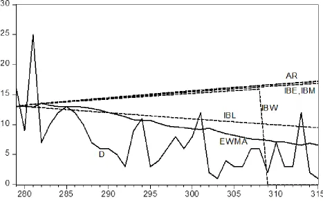
<< Insert Figure 5 about here. >>
Figure 5 shows time plots for the observed EOL phase of actual demand and its EWMA smoothed version (solid lines), and the five alternative forecasts (dotted lines). IBL is clearly doing best and is rather successful in tracking the EWMA series that was used to estimate the model. The real interest lies in forecasting actual demand over the EOL phase, and IBL is also the best method in this respect. The models for IBW, IBE, and IBM provide forecasts that are nearly identical to that of the black box model, which is explained by the lack of significance of mean age in these models. The actual total demand over the observed EOL phase is 247, and the predicted totals are as follows: 551 (AR), 404 (IBL), 424 (IBW), 552 (IBE), and 545 (IBM). The relative total error, defined by SUM in (6), is 0.64 (IBL), 0.72 (IBW), 1.21 (IBM), 1.23 (IBE), and 1.23 (AR). IBL provides the best forecasts also in this respect, with IBW as second-best. This ranking is confirmed by the criteria MAPE (0.77 for IBL, 1.05 for IBW, 1.21 for IBE, 1.30 for IBM, 1.33 for AR) and RMSPE (0.87 for IBL, 1.21 for IBW, 1.44 for IBM, 1.46 for IBE, and 1.46 for AR).
Our conclusion is that lifetime installed base provides helpful information to forecast spare part demand for the relatively expensive and essential compressors for this type of refrigerator, which is a non-trendy product with long lifecycle. As compared to black box forecasting, the error in total EOL demand is reduced by a factor of about two (from 304 to 157). These results confirm our first and second research hypotheses formulated in Section 2.3.
5 Results for three types of consumer products
5.1Overview of eighteen spare parts
15
refrigerators (top row), televisions (middle row), and smartphones (bottom row). IBE and IBM depend on the (cost of the) spare part, and Figure 6 shows these two types of installed base for the most expensive spare part per product. The top left graph is identical to Figure 3.
Some characteristics of the products and spare parts are summarized in Table 1. The price of spare parts does not incorporate handling and labor costs. These additional costs are rather marginal for televisions and smartphones, because customers can easily bring these products to repair shops. The labor costs are more substantial for refrigerators, because their repair requires that a skilled technician visits the owner at home. Table 1 also shows our hypothesis on which installed base is expected to be most useful in forecasting EOL demand. The motivation for each of these hypotheses is described below in Sections 5.2-5.4, together with the main forecast results for the eighteen spare parts. Further details on models and forecasts are available from the authors upon request.
<< Insert Figure 6 about here. >>
<< Insert Table 1 about here. >>
5.2Refrigerator spare parts demand
Refrigerators have a long lifecycle, and Table 1 shows that the forecast evaluation period covers only a small part of the full EOL phase. The product warranty lasts for two years.
An essential and expensive spare part is the compressor (price 14-18% of that of the refrigerator). As was explained in Section 4.1, we expect IBL to perform best for this spare part, because repairing the compressor provides large gains in expected lifetime and refrigerators do not quickly get out of fashion. An expensive and non-essential part is the circuit board (relative price 6-8%). The refrigerator works well even if some functions of the circuit board have broken down. As the product has a much longer lifetime than the warranty period and keeps high utility until end of life, our third hypothesis in Section 2.3 suggests that consumers make economic decisions and replace this non-essential part if the remaining value of the refrigerator, which has a long lifecycle, is higher than the replacement costs. That is, we expect that IBE will provide the best forecasts. A cheap and non-essential spare part is the door gasket (relative price about 3.5%). Even though this spare part is relatively cheap, replacement by the manufacturer is costly as a specialized repairer should visit the owner at home. We therefore expect consumers to demand this spare part only during the warranty period and to find other solutions after warranty has expired. That is, we expect IBW to provide the best forecasts.
16
that IBE performs best is confirmed for the first type of refrigerator, but not for the second type where black box forecasts are much better. The cause of the bad forecast performance of IBE in the latter case is that the model has a significant positive coefficient for mean age, which increases steadily over EOL, whereas actual EOL demand is rather stable. Note that this bad forecast performance could not be foreseen at the start of the EOL phase, as the future trends in spare part demand have somehow to be extrapolated from the past. The results for the door gasket are varied, as our hypothesis that IBW is best is confirmed for the second type of refrigerator, but not for the first type where IBM performs better. Overall, the outcomes provide support for the first and second hypotheses of Section 2.3 on the value of installed base forecasting and the usefulness of lifetime and warranty installed base, and partial support for the third hypothesis on the usefulness of economic installed base.
<< Insert Table 2 about here. >>
5.3Television spare parts demand
High-tech products, like televisions, experience decreasing lifecycles because of fast innovations and quickly developing consumer trends (Pourakbar et al., 2012, 2014). Consumers tend to base their buying decisions for these products less on economic value and more on the wish to own new product features. Therefore, the value of these products as experienced by consumers often decays much faster than the economic lifecycle would suggest. Because of the shortened lifecycle due to innovations, we expect that warranty installed base for these products is in general more informative than lifetime and economic installed base. The warranty period is two years.
Both types of flat screen televisions have very short sales periods of approximately one year. The estimation period for all models is too short to provide reliable forecasts. All methods, including black box, are far off the mark. We conclude that full EOL forecasting after such a short estimation period is too challenging, and instead we consider the more modest task to forecast remaining EOL demand one year after the end of product sales. The estimation period then becomes about two years, and the forecast evaluation period is about three years for television type 1 and about two years for type 2, as type 2 was introduced about one year after type 1.
17
is again expected to give the best forecasts.
Table 3 shows the forecast results for television spare parts. Most of the outcomes support our hypotheses, as IBW provides the best EOL demand forecasts in five out of six cases. The only exception is found for circuit boards for the first type of television, where IBE and IBL do slightly better. The differences between the four installed base types are small for this specific spare part, and each of these four methods is considerably better than the black box method. The outcomes therefore support our first and second hypotheses of Section 2.3 on the usefulness of warranty installed base for products with short lifecycle.
<< Insert Table 3 about here. >>
5.4Smartphone spare parts demand
The market for smartphones has expanded very rapidly in recent years. Consumers are fast in adopting new technologies, as product innovations expand the functionalities of new phones. Giachetti and Marchi (2010) find that this market is highly competitive, not only between brands but also between products of the same brand. The continuous launch of innovative technologies in the global mobile phone industry stimulates replacing old phones by new ones and reduces spare part demand. The two smartphones in our case study are of the same brand. The first type is an early version, which is followed up within a year of its introduction by a second type that has much better functionalities. Both phones have a warranty period of two years, and the second type is introduced before the warranty period of the first type has expired. The far majority of phones is sold by telecom companies in combination with mandatory financial and maintenance contracts that last for one or two years. Consumers with such contracts are forced to use the product during this mandatory period, irrespective of their subjective evaluation of the remaining product value. We therefore expect that owners of the first type of phone will demand spare parts only during the warranty period, as later on they will wish to switch to the much improved new version. The second type of phone is still up-to-date and fashionable after the warranty period, and late adopters can continue using this phone whereas early adopters will move to newer products. We therefore expect that consumer decisions for the second phone will be mixed. Summarizing, we expect in general that IBW will be the best method for the first phone, and IBM for the second one.
18
price 1-2%). As this part is so cheap and very easy to buy at shops or via internet, we expect that the demand for this spare part is best predicted by IBL.
Table 4 shows the forecast results for smartphone spare parts. Our hypotheses for the circuit board are confirmed, as IBW is clearly the best for phone 1 and IBM for phone 2. IBW is also best for touch screens, and this confirms our hypothesis for phone 1 but not for phone 2. The outcomes show that users of both phones replace the touch screen mostly during the warranty period. IBW is also best for back covers, contrary to our expectation that this cheap spare part would be replaced also after warranty has expired. Smartphone users seem not to wish repairing cosmetic parts after warranty has expired, even if the spare part is cheap. Overall, the outcomes provide support for the first hypothesis of Section 2.3, and partial support for the second and fourth hypothesis on the usefulness of the various considered installed base types.
<< Insert Table 4 about here. >>
5.5 Theoretical and practical contributions of the study
The main theoretical contribution of our study lies in proposing installed base concepts that are practically viable for B2C companies. The use of installed base in demand forecasting is currently limited to advanced companies in a B2B environment, whereas B2C companies still tend to simply extrapolate past demand patterns. The demand for products of B2B companies often originates from long-term delivery and maintenance contracts with large clients that provide them with reliable operational information on the number of products in use. Even though B2C managers usually lack such detailed information, our study shows that such managers can substantially improve their consumer demand forecasts by employing installed base concepts (lifetime, warranty, economic, and mixed) that can be constructed from the management information available to them. The main question of interest to B2C managers then is which type of installed base gives the best information. We present and test a set of hypotheses on which type of installed base works best for which type of consumer products. The proposed hypotheses are based on characteristics of the product (such as life cycle length and innovation speed) and of the spare part (such as ease of repair and price of spare part relative to price of new product) as well as on product-specific consumer attitudes (such as sensitivity to innovations).
19
errors over the EOL phase. Their test provides automatic correction for the extensive serial correlation that is present in the weekly series of forecast errors. If our hypothesis is confirmed, then we test whether this method is significantly better than the second-best method as measured by the SUM and MAPE criteria. If our hypothesis is denied, then we test whether the best method is significantly better than the method of the hypothesis. Small p-values indicate that one method is significantly better than the other. The final column in Table 5 shows whether our hypothesis is significantly confirmed or denied by the two tests. Confirmation is found in twelve out of eighteen cases, whereas denial occurs in six cases. Possible causes of these denials were discussed in previous sections.
<< Insert Table 5 about here. >>
We summarize our empirical findings in terms of the four hypotheses of Section 2.3. The first hypothesis, that installed base forecasts are better than the considered black box AR methods, is confirmed for seventeen out of the eighteen spare parts in Table 5, and Tables 2-4 show that the improvements are substantial. The second hypothesis concerns the relative performance of lifetime and warranty installed base. Table 5 shows that one of these two installed bases is expected to be best for fourteen spare parts, and the hypothesis is confirmed for ten of these spare parts. The most notable exception occurs for back covers of smartphones, where the outcome that IBW is better than IBL is reverse to what was expected. The third hypothesis is on economic installed base, which is our hypothesis for one spare part of refrigerators. This hypothesis is confirmed for one type of refrigerator but not for the other type. The fourth hypothesis is on mixed economic installed base, which is our hypothesis for two spare parts of smartphone type 2. This hypothesis is confirmed for one of these spare parts, but not for the other one.
A final note for practitioners is that EOL demand forecasting is only feasible provided that the learning period consisting of the initial and mature phases is long enough. This condition holds equally well for simple extrapolation methods and for installed base forecasts, as both methods require product-specific information on demand patterns.
6 Conclusions
20
characteristics of the product, the spare part, and the consumer market. Warranty installed base is advised for spare parts with relatively short lifecycle, and lifetime installed base for essential spare parts for products with long average lifetimes. Economic installed base is useful for non-essential spare parts of products with long average lifetimes that are out of warranty. If consumers differ in their adoption attitudes for product innovations, a mixed economic installed base can be useful. Our case study shows that installed base forecasts improve much upon straightforward black box autoregressive extrapolation of past demand patterns.
Although the specific results will vary across products, the proposed methodology is technically viable to forecast EOL spare part demand for any product. The required information for each product and spare part is the following. First, and most important, time series of product sales and of spare part demand until start of EOL. Further, the average lifetime of the product (for lifetime installed base), the warranty period (for warranty installed base), the cost of the spare part (for economic installed base), and consumer segments (for mixed economic base). We propose to smooth the demand data after screening them for extreme values that may occur, for example, in case of extraordinary failure rates briefly after introduction of a new product. The quality of the forecasts depends on the richness of the available data, ideally with a long estimation period during the production phase and with a limited EOL phase. In practice, the production period is often relatively short as compared to the EOL phase, and this also applies for the products in our case study. We advise to use simple models in such cases, in order to prevent forecast deterioration due to over-fitting. We do not advise a fully automated forecast procedure, because consumer behavior differs widely across products. It can be helpful to cluster products and spare parts in groups, depending on their characteristics and on expected consumer demand behavior. Within each cluster, EOL spare part demand can be forecasted by using one common type of installed base that applies for all products of that cluster.
References
Auramo, J., & Ala-Risku, T. (2005). Challenges for doing downstream. International Journal of Logistics: Research and Applications, 8, 333–345.
Bacchetti, A., & Saccani, N. (2012). Spare parts classification and demands forecasting for stock control: investigating the gap between research and practice. Omega, 40, 722-737.
Box, G.E.P., & Jenkins, G.M. (1976). Time series analysis, forecasting and control. (2nd ed.). San Francisco: Holden-Day.
Boylan, J.E., & Syntetos, A.A (2009). Spare parts management: a review of forecasting research and extensions. IMA Journal of Management Mathematics, 21, 227-237.
21
Chou, Y.C, Hsu, Y.S., & Lin, H.C. (2015). Installed base forecast for final ordering of automobile service parts. International Journal of Information and Management Sciences, 26, 13-28.
Cohen, M.A., Kamesam, P.V., Kleindorfer, P., Lee, H., & Tekerian, A. (1990). Optimizer: IBM’s multi-echelon inventory system for managing service logistics. Interfaces, 20, 65–82. Dekker, R., Pince, C., Zuidwijk, R., & Jalil, M.N. (2013). On the use of installed base information for spare parts logistics: a review of ideas and industry practice. International Journal of Production Economics, 143, 536-545.
Diebold, F.X., & Mariano, R.S. (1995). Comparing predictive accuracy. Journal of Business and Economic Statistics, 13, 253-263.
Entner, R. (2011). International comparisons: the handset replacement cycle. Report Recon Analytics. June 23, 2011.
Giachetti, C., & Marchi, G. (2010). Evolution of firms’ product strategy over the life cycle of technology-based industries: A case study of the global mobile phone industry, 1980–2009. Business History, 52, 1123–1150.
Hong, J.S., Koo, H.Y., Lee, C.S., & Ahn, J. (2008). Forecasting service parts demand for a discontinued product. IIE Transactions, 40, 640–649.
Inderfurth, K., & Mukherjee, K. (2008). Decision support for spare parts acquisition in post product life cycle. Central European Journal of Operations Research, 16, 17-42.
Islam, T., & Meade, N. (2000). Modelling diffusion and replacement. European Journal of Operational Research, 125, 551-570.
Jalil, M.N., Zuidwijk, R., & Fleischmann, M. (2011). Spare parts logistics and installed base information. Journal of the Operational Research Society, 62, 442-457.
Jin, T., & Liao, H. (2009). Spare parts inventory control considering stochastic growth of an installed base. Computers and Industrial Engineering, 56, 452–460.
Jin, T., Liao, H., Xiong, Z., & Sung, C. H. (2006). Computerized repairable inventory management with reliability growth and increased product population. In Proceedings of Conference on Automation Science Engineering, October 8–9, 2006, Shanghai, China.
Jin, T., & Tian, Y. (2012). Optimizing reliability and service parts logistics for a time-varying installed base. European Journal of Operational Research, 218, 152-162.
JP Morgan Inc. (1996). RiskMetrics. Technical document (4-th ed.). New York.
Kim, B., & Park, S. (2008). Optimal pricing, EOL (end of life) warranty, and spare parts manufacturing strategy amid product transition. European Journal of Operation Research, 188, 723-745.
Minner, S. (2011). Forecasting and inventory management for spare parts: An installed base approach. In S.N. Altay, & L.A. Litteral (Eds.), Service Parts Management (pp. 157-169). Berlin: Springer-Verlag.
22
National Purchase Diary Display Search. (2012). Global TV replacement study. Report. California: Santa Clara. May 29, 2012.
Pince, C., & Dekker, R. (2011). An inventory model for slow moving items subject to obsolescence. European Journal of Operational Research, 213, 83-95.
Pourakbar, M., Frenk, J. B. G., & Dekker, R. (2012). End-of-life inventory decisions for consumer electronics service parts. Production and Operations Management, 21, 889–906. Pourakbar, M., Van der Laan, M., & Dekker, R. (2014) End-of-life inventory problem with phase-out returns. Production Operations Management, 23, 1561–1576.
Rogers, E.M. (2003). Diffusion of innovations (5th ed.). New York: Free Press.
Teunter, R., & Fortuin, L. (1998). End of life service: a case study. European Journal of Operational Research, 107, 19-34.
Teunter, R.H., Syntetos, A.A., & Babai, M.Z. (2011). Intermittent demand: linking forecasting to inventory obsolescence. European Journal of Operational Research, 214, 606-615.
Tibben-Lemke, R.S., & Amato, H.N. (2001). Replacement parts management: The value of information. Journal of Business Logistics, 22, 149-64.
Van der Heijden, M., & Iskandar, B.P. (2013). Last time buy decisions for products sold under warranty. European Journal of Operational Research, 224, 302-312.
Wagner, S.M., & Lindemann, E. (2008). A case study-based analysis of spare parts management in the engineering industry. Production Planning and Control, 19(4), 397-407.
23
24
25
26
Figure 4: Demand for compressor of refrigerator type 1: time series of actual and EWMA smoothed demand against time in weeks (top left), and three scatter diagrams of smoothed demand in units on vertical axis against installed base in 1,000 units on horizontal axis, for lifetime installed base (top right), warranty installed base (bottom left), and economic installed base (bottom right)
0 50 100 150 200 250
25 50 75 100 125 150 175 200 225 250 275 300 EOL Init Mat 0 10 20 30 40 50 60
0 100 200 300 400 500 600
IBL X X Mat EOL Init unit:K 0 10 20 30 40 50 60
0 100 200 300 400 500
IBW Init EOL Mat X X Unit:K 0 10 20 30 40 50 60
0 100 200 300 400 500
27
28
Figure 6: Time series of installed base in 1,000 units on vertical axis against time in weeks on horizontal axis for six products: refrigerators (top row), televisions (middle row), and
smartphones (bottom row), for type 1 (left column) and type 2 (right column); in each diagram, the vertical line indicates the start of the end-of-life phase
0 100 200 300 400 500 600
25 50 75 100 125 150 175 200 225 250 275 300 IBL IBE IBM IBW EOL (a) Unit:K 0 40 80 120 160 200
25 50 75 100 125 150 175 200 225 250 275 (b) EOL IBL IBE IBM IBW Unit:K 0 5 10 15 20 25 30 35 40
25 50 75 100 125 150 175 200 225 250 (c) EOL IBL IBW IBM IBE Unit:K 0 10 20 30 40 50 60
25 50 75 100 125 150 175 200 (d) IBL IBE IBW IBM EOL Unit:K 0 50 100 150 200 250 300 350 400
25 50 75 100 125 150 175 (e) EOL IBL IBW IBE IBM Unit:K 0 100 200 300 400 500 600 700 800
29 Table 1: Overview of six products and eighteen spare parts
Product Estim. Forec. Lifecycle
Life cycle Tech trendy
Refrigerator 1 Long Low 08.12 - 13.29 279 36 676
Refrigerator 2 Long Low 08.32 - 12.51 229 66 676
Television 1 Short Low 09.23 - 10.17 100 152 360
Television 2 Short Low 10.12 - 11.15 108 102 360
Smartphone 1 Short High 10.24 - 11.28 109 89 160
Smartphone 2 Short High 11.19 - 13.04 90 61 160
Spare part Essential Expensive Hypothesis
1 2 1 2 1 2
For refrigerator
Compressor Yes Yes 5,678 6,090 4.4 13.6 46.7 39.8 L
Circuit board No Yes 9,596 3,518 17.7 36.5 7.6 5.6 E
Door gasket No No 4,581 698 17.7 10.0 3.5 3.4 W
For television
LCD panel Yes Yes 868 889 24.9 20.6 47.0 39.4 W
Circuit board No Yes 562 774 37.7 39.1 9.6 8.2 W
Cover No No 152 230 9.2 16.1 3.2 4.5 W
For smartphone
Touch screen Yes Yes 21,499 58,413 16.5 23.8 19.8 25.8 1W, 2M
Circuit board No Yes 6,325 14,492 14.2 37.6 28.6 40.0 1W, 2M
Back cover No No 5,259 11,033 42.4 45.8 1.6 1.2 L
Table notes
* Consumer sentiments describe aspects that affect consumer attidudes towards products and spare parts. * Sales is total product sales during sales period, indicated in format year.week (e.g., 08.12 is week 12 of 2008). * Estim. and Forec. show number of weeks of data available respectively for estimation and for forecast analysis. * Lifecycle is average lifetime in weeks, obtained for refrigerators from National Association of Home Builders
(2007), for televisions from NPD DisplaySearch (2012), and for smartphones from Entner (2011). * "Essential" describes whether spare part is essential for product, and "Expensive" indicates relative price of
spare part compared to product price (excluding spare part repair costs if service engineer is needed). * Demand is total spare part demand until analysis date, i.e., week 13 of 2014, for products of type 1 and type 2. * EOL % shows demand during EOL phase as percentage of demand in initial and mature phases.
* Price % is price of spart part as percentage of product price, for type 1 & for type 2.
* Hypothesis shows installed base hypothesis for the spare part (L for IBL, W for IBW, E for IBE, M for IBM). 50,986
348,153 694,816
Demand EOL % Price %
Consumer sentiments Sales Period
30 Table 2: Forecast results for refrigerator spare parts
Spare part
AR L W E M
1, Compressor
SUM 1.23 0.64 0.72 1.23 1.21
MAPE 1.33 0.77 1.05 1.21 1.30
RMSPE 1.46 0.87 1.21 1.46 1.44
2, Compressor
SUM 0.81 0.05 0.32 0.17 0.12
MAPE 0.98 0.49 0.62 0.53 0.52
RMSPE 1.08 0.68 0.75 0.69 0.69
1, Circuit board
SUM -0.10 0.03 -0.13 -0.01 0.03
MAPE 0.27 0.25 0.39 0.25 0.25
RMSPE 0.32 0.32 0.54 0.31 0.32
2, Circuit board
SUM -0.09 3.04 -0.27 2.94 1.37
MAPE 0.27 3.09 0.37 2.99 1.43
RMSPE 0.36 4.07 0.48 3.93 1.68
1, Door gasket
SUM -0.08 0.09 -0.15 0.07 0.05
MAPE 0.38 0.47 0.43 0.45 0.44
RMSPE 0.59 0.62 0.61 0.61 0.61
2, Door gasket
SUM 1.43 0.18 0.07 0.17 0.19
MAPE 1.60 0.94 0.85 0.94 0.94
RMSPE 1.79 1.13 1.13 1.13 1.13
Table notes
* The two types of refrigerator are denoted by 1 and 2.
* Installed base L denotes lifetime, W warranty, E economic, and M mixed economic. * SUM is the summed forecast error over observed EOL as fraction of EOL demand; a positive (negative) value corresponds to over-forecasting (under-forecasting) actual demand. * RMSPE and MAPE are respectively the root mean weekly squared prediction error and the mean weekly absolute prediction error over observed EOL, each as fraction of the mean weekly EOL demand.
31 Table 3: Forecast results for television spare parts
Spare part
AR L W E M
1, LCD panel
SUM 4.60 22.03 -0.22 -1.00 -1.00
MAPE 4.64 22.03 0.89 0.99 1.00
RMSPE 4.79 24.42 1.48 1.76 1.76
2, LCD panel
SUM 3.45 0.48 0.46 -1.00 -1.00
MAPE 3.46 0.78 0.95 1.00 1.00
RMSPE 3.73 1.00 1.34 1.39 1.39
1, Circuit board
SUM 2.31 -0.16 -0.26 -0.03 0.15
MAPE 2.52 0.65 0.68 0.72 0.74
RMSPE 2.75 0.92 0.98 0.98 0.95
2, Circuit board
SUM 6.26 7.55 0.85 5.77 8.03
MAPE 6.26 7.54 1.48 5.82 8.05
RMSPE 7.37 9.06 1.95 7.68 9.56
1, Cover
SUM 13.86 5.86 1.20 3.58 3.62
MAPE 14.11 6.51 2.17 4.34 6.51
RMSPE 14.11 7.60 4.34 5.43 7.60
2, Cover
SUM 4.45 3.53 0.25 2.40 2.01
MAPE 4.69 3.86 1.38 2.76 2.48
RMSPE 5.24 4.14 2.76 3.31 3.31
Table notes
* This table is similar to Table 2.
* Spare part demand forecasts are not for the full EOL phase, but for the subperiod starting one year (52 weeks) after begin of EOL.
32 Table 4: Forecast results for smartphone spare parts
Spare part
AR L W E M
1, Circuit board
SUM 6.03 4.04 -0.05 -1.00 -1.00
MAPE 6.05 4.08 0.96 1.00 1.00
RMSPE 6.34 4.66 1.76 2.05 2.05
2, Circuit board
SUM 0.71 0.78 0.76 -0.24 0.03
MAPE 0.85 0.91 0.89 0.73 0.69
RMSPE 0.99 1.06 1.03 0.93 0.86
1, Touch screen
SUM 5.03 3.01 -0.31 0.97 2.20
MAPE 5.18 3.16 0.65 1.37 2.44
RMSPE 5.36 3.62 1.25 2.08 2.96
2, Touch screen
SUM 1.74 0.54 0.36 1.15 -0.45
MAPE 1.77 0.65 0.67 1.26 0.88
RMSPE 1.89 0.80 0.91 1.41 1.15
1, Back cover
SUM 3.53 4.46 0.83 5.74 5.69
MAPE 3.84 4.76 1.59 6.03 5.99
RMSPE 4.14 5.18 2.07 6.88 6.98
2, Back cover
SUM 0.42 1.88 0.18 0.70 1.13
MAPE 0.86 2.17 0.67 1.08 1.49
RMSPE 1.13 2.51 0.99 1.25 1.79
Table notes
* This table is similar to Table 2.
* Forecast evaluation period is full EOL phase for smartphone type 2, and subperiod starting one year (52 weeks) after begin of EOL for smartphone type 1.
33 Table 5: Evaluation of forecast strategies
Spare part Hypothesis Outcome Conclusion
Type SUM MAPE
Refrigerator
1, Compressor L L L > W 0.000 0.000 Confirmed (2x)
2, Compressor L L L > M 0.000 0.006 Confirmed (2x)
1, Circuit board E E E > L 0.000 0.400 Confirmed (1x)
2, Circuit board E AR AR > E 0.000 0.000 Denied (2x)
1, Door gasket W M M > W 0.001 0.855 Denied (1x)
2, Door gasket W W W > E 0.000 0.293 Confirmed (1x)
Television
1, LCD panel W W W > E 0.000 0.000 Confirmed (2x)
2, LCD panel W W W > L 0.378 0.995 Weakly confirmed (1x)
1, Circuit board W E E > W 0.000 0.802 Denied (1x)
2, Circuit board W W W > E 0.000 0.000 Confirmed (2x)
1, Cover W W W > E 0.000 0.000 Confirmed (2x)
2, Cover W W W > M 0.000 0.000 Confirmed (2x)
Smartphone
1, Circuit board W W W > E 0.000 0.400 Confirmed (1x)
2, Circuit board M M M > E 0.001 0.228 Confirmed (1x)
1, Touch screen W W W > E 0.000 0.000 Confirmed (2x)
2, Touch screen M W W > M 0.000 0.021 Denied (2x)
1, Back cover L W W > L 0.000 0.000 Denied (2x)
2, Back cover L W W > L 0.000 0.000 Denied (2x)
Table notes
* Hypothesis on installed base: lifetime L, warranty W, economic E, or mixed economic M. * Outcome shows the installed base that provides the best forecasts (taken from Tables 2-4); if best method varies across criteria, then method with best SUM is taken as outcome.
* Test type A > B tests whether method A provides better forecasts than method B; if the outcome confirms the hypothesis, then A is the hypothesis and B is second-best method (with respect to SUM); if the outcome differs from the hypothesis, then A is the outcome and B is the hypothesis. * Test SUM is t-test for mean error, and MAPE is Diebold-Mariano test for absolute errors; the table shows the p-value for the one-sided alternative that base A is better than base B. * Conclusion "confirmed" denotes that the hypothesis base is significantly better (for 1 or 2 tests) than second-best; "weakly confirmed" means that hypothesis base is best, but not significantly better than the second-best base; "denied" means that the hypothesis base performs significantly worse than the best base; significance level is 5%.