Stability and Robust Performance Analysis of Fractional Order Controller over Conventional Controller Design

Please cite this article as: P. Kumar, S. Kumar Chaudhary, Stability and Robust Performance Analysis of Fractional Order Controller over Conventional Controller Design,International Journal of Engineering (IJE),IJE TRANSACTIONS B: Applications Vol. 31, No. 2, (February 2018) 322-330

International Journal of Engineering

Stability and Robust Performance Analysis of Fractional Order Controller over

Conventional Controller Design

P. Kumar*, S. Kumar Chaudhary

Electrical Engineering Department, SunRise University, Alwar, Rajasthan, India

P A P E R I N F O

Paper history: Received 12May2017

Received in revised form 15June2017 Accepted 12October2017

Keywords:

Fractional Order Controller Fractional Order Calculus Stability

Performance Analysis Function Under Class Ziegler-Nichols Method

A B S T R A C T

In this paper, a new comparative approach was proposed for reliable controller design. Scientists and engineers are often confronted with the analysis, design, and synthesis of real-life problems. The first step in such studies is the development of a 'mathematical model' which can be considered as a substitute for the real problem. The mathematical model is used here as a plant. Fractional integrals and derivatives have found wide application in the control of dynamical systems when the controlled system and the controller are described by a set of fractional order differential equations. Here the stability and robustness of fractional order system is checked at the different level and it is found that the stability region is large in the complex plane. This large stability region provides the more flexibility for system implementation in the control engineering. Generally, an analytically or experimentally approaches are used for designing the controller. If a fractional order controller design approach used for a given plant then the controlled parameter gives the better result.

doi: 10.5829/ije.2018.31.02b.17

1. INTRODUCTION1

The technique model order reduction is used in all fields of electrical, chemical, aerospace, mechanical etc. In the large process control system and mechanical production houses, the model order reduction plays an important role to take the decision for the final product [1-3]. Generally, the work with large scale system is very complex and time-consuming [4]. To check the stability of the system first we make a mathematical model of the plant. If the original system model does not match the desired performance of the implementing system, then a controller is designed to fulfill the requirement of the industry. The designed controller may be a full order or it may be fractional order. The implementation of the controller depends on the plant. If a control system satisfies their stability conditions by the Routh-Hurwitz stability criteria [5] then any analytical or experimental approaches are used. On the other hand, if control system requires the stability region beyond the Routh-Hurwitz criteria or it requires more flexibility [6-9] than

*Corresponding Author’s Email:[email protected](P. Kumar)

what an approach is useful? So to fulfill the stability condition beyond the Routh- Hurwitz criteria a fractional order approach [10, 11] is used here to design the controller. Here the comparative analysis provides the option to opt a controller design method for the given plant.

2. PID CONTROLLER TRANSFER FUNCTION

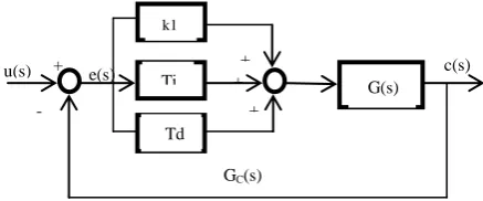
The block diagram for a PID controller is shown in Figure 1. The PID controller may be represented in mathematical form as follows:

] ) ( 0 ()

1 ) ( [

1 ) (

dt t de t

d T d t e i T t e

k t

u   _  (1)

] 1 1 [ )

( 1 T s

s T k s G d i

c    (2)

Equation (2) can be rewritten as

s k s k k s

G_c( ) ₁ 2  ₃ (3)

Here k2and k3 used for integral gain and derivative gain values of the controller respectively.

The objective is to derive a controller such that the performance of the augmented process matches with the desired performance of the model. In the computational system, the desired performance should be satisfied by the closed loop control system [12, 13]. To fulfill these entire requirements a PID controller is derived in form of full order and fractional order.

3. FRACTIONAL ORDER SYSTEM FUNDAMENTALS

3.1. Introduction to Fractional Calculus The term “fractional-order calculus” is not new. It is a generalization of ordinary differentiation by non-integer derivatives. The theory of fractional-order derivatives was mainly developed in 19th century [14-17]. In the development of fractional order calculus, there appeared different definitions of fractional-order differentiation and integration [18, 19]. To reduce to a general form fractional calculus from integration and differentiation to the fractional order fundamental operatorD_tf(t), where α and t are the limit and R is the directive of operation. The continuous integration differential operator is [20]:

            



There are various definitions for fractional integration and differentiation. Some of the definitions spread out directly as of integer-order calculus.The deep-rooted descriptions include the Cauchy integral formula, the Grunwald–Letnikov (GL) definition and Riemann– Liouville (RL) definitions are given [20] as:

Definition 1: - Cauchy integral formula

Figure 1. PID controller block diagram



( (5)

where, c is the smooth curve encircling the single value function f (t)

Definition 2: - Grunwald–Letnikov (GL) definition:

) ( ) 1 ( 0 ) ( 0 jh t f j h h Lim t f D h t j j

t  

       



Here the term in [.] represent the integer part. Definition 3: - Riemann-Liouville (RL) definition:



The following function given below is obtained by Laplace Transform of the GL and RL fractional differential-integral. The zero initial conditions and order gives the following result:

) ( ]

); (

[ Dt f t s s F s

 

  _ 

 (8)

3.2. Fractional Order System The fractional-order system is the extension form of the traditional integer order systems. Fractional order system is gained from the fractional-order differential equations. A classic n-term linear fractional order differential equation (FODE) is assumed by:

Let considering the control function on which input signal is applied to FODE system Equation (9) as follows: ) ( ) ( ) ( ... )

( 0 0

1

1 yt ut

t D t y t D t y D n t

n    

      (10)

After Laplace transform of Equation (10), we get:

) ( ) ( ) ( ... )

( ₁ 1 ₀ 0Y t U t

t s t Y t s t Y s n t

n    

      (11)

From Equation (11), we can obtain a fractional-order transfer function as

n s s s s U s Y s G n    _{ }       .. 1 ) ( ) ( ) ( 1 0 1 0 (12)

In broad, for a dynamic system with single variable and fractional order transfer function of a system can be defined as: n m s a s a s a s b s b s b s G n y m             ... ... ) ( 1 0 1 0 1 0 1 0 (13)

Here b_i(i0,1...m),a_i(i0,1...n)are constant and ) ... 1 , 0 ( ), ... 1 , 0

(i m ii n

i   

 are random real or rational

0 ) ( ) ( ... )

(   ₁ 1  ₀ 0yt  t D t y t D t y D n t n       (9) -+

u(s) e(s) c(s)

+ +

+

G(s)

GC(s) k1

Ti

number and without lacking generality, can be

prescribed asm m1...0andm m1...0_. The incommensurable fractional order system Equation (13) can also be expressed incommensurable form by the multi-valued transfer function:

). 1 ( ,

... ... )

(

1

1 0

1

1

0 _

  

  

 v

s a s a s a

s b s b s b s H

v n

n v

v m

m v

(14)

Note that every fractional order system may be represented in the form of Equation (14) and domain of H(s) meaning is a Riemann sheets.

4. STABILITY OF FRACTIONAL ORDER SYSTEM

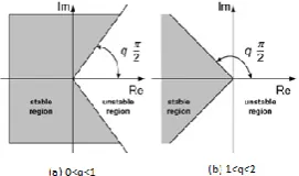
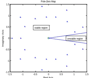
Stability is one of the most frequent terms used in literature when we deal with the dynamical systems and their behaviors. In mathematical vocabulary, stability theory addresses the convergence clarifications of differential or difference equations. A system (LTI) is said to be stable if the roots of characteristics polynomial had negative real part. In the case of fractional order system (LTI), the stability is not same as of integer one. Important point is that, for a fractional order system, the roots may lie on the right half of complex plane Figure 2.

Theorem: - According to Matignon’s stability theorem the fractional order transfer function

) (

) ( ) (

s D

s N s

G 

is stable if and only if

2 )

arg(i q , where

q

s



 ,

(0<q<2) with_iC, th

i _{root of}

. 0 ) (  D

Ifs0, is a single root of D(s), the system cannot be stable.

Above theorem stability region is shown in Figure 2, Indicate the wholes s plane whereq0. It shows the Routh-Hurwitz stability and q1 tends to the negative real axis forq2.

As we know that only the poles play an important role in the stability of a system. So the stability assessment is done by denominator only and numerator does not affect the stability of an FOTF.

Figure 2. Stable and unstable region of LTI fractional order system

The stability of fractional order system can be analyzed in another way also. Let considering here, the characteristic equation of a general fractional order system as:

0 ...

0 1

0 0  1  





i

s s

s s

n

i i n n

 



 _{  }

 (15)

For v v_i i 

 , we can transform the Equation (15) into the

σ-plane.

0

0

 





 

i i

v n

o i

i v v n

i

is 

 (16)

Here m

k

s



 and m is the least common multiple of ѵ. For a given αi, if the absolute phase of all roots of transform Equation (16) is_  arg(), we can close the following points for the stability of fractional order systems.

1. The stability condition is as _{arg( ) .}

2m m

 

 _{ }

2. The oscillation condition is as _.

2 ) arg(

m

  

If any linear time invariant (LTI) fractional order system satisfy the above two points then the system is stable otherwise unstable.

5. FRACTIONAL ORDER CONTROLLER DESIGN

Maximum of the works in fractional order control systems are in hypothetical nature. Controller design and application in run-through is very small. In this paper, the core objective is to spread on the fractional order control (FOC) to examine the system control performance. The fractional-order PIλDμ controller was proposed as a broad view of the PID controller with integrator of real order λ and differentiator of real order μ. The transfer function of such kind the controller in Laplace domain has form:

) 0 , ( , )

(   _ K s   s

K K s

C P I D (17)

Here KP is the proportional gain constant KI is the integral gain constant and KD is the derivative gain constant. If λ=1and μ=1, we obtained a classical PID controller. If λ=0 and μ=0, we obtained a PDμ and PIλ controller respectively. These entire controllers are the case of PIλDμ controller, which provides flexibility with an opportunity to adjust the dynamic property of fractional order control system. Two steps are used here to design such controllers.

Step 1: - Design of KP

      

t P

E

K 100 (18)

Here Proportional gain KP is selected for minimum static error.

Step 2: - Design of KD, μ, KI and λ

To determine these values for Fractional-Order controller design, the following synthesis scheme is used here.

Let the controller transfer function is C(s), plant transfer function is G(s) and a unity feedback is applied to the system. Phase margin of controlled system [21, 22] is:







_m argC(j _g)G(j _g) ₍₁₉₎

Here jωg is the crossover frequency. Phase margin is an independent or constant phase. This can be accomplished by controller of the form:



 



 1 2

2

1 ,

1 ,

1 )

( k

K k s

s k k s C

plant

v (20)

Here Kplant is the gain of plant and τ is the time constant for the plant.

Now from Equations (19) and (20)









  

   

 

  

 

         

 

 



2 ) 1 (

) ( arg

arg

) ( ) ( arg

) 1 (

) 1 ( 1

 

 

 

   

v j

j k k

j G j C

v v plant

g g m

(21)

Here for a given plant, we fix the gain margin. Put the gain value in Equation (21) one can find out the value of v. the other desired values k1 and k2 are obtained from Equation (20).

Now using these constant in Equation (20), we can obtain a fractional IλDμ controller, which is a particular case of PIλDμ controller has the form

1 2

1 1

) 1 ( 2

1 ;

)

(s k k s k s K k k andK k

C D I

v

v _{  }

  

(22)

If the value of KP is given then the full transfer function of fractional order controller is

v I v D

P K s K s

K s

C( )  (1)  (23)

If do a comparison with Equation(17), we can say v

and

v 



 

 (1 ) _.

6. CONTROLLER DESIGN USING ZIEGLER-NICHOLS SECOND METHOD

In this method, we first set T= ∞and T_d= 0. By using the proportional control action increase Kfrom 0 to a critical valueK_crat which the output exhibits sustained oscillations in the system.

Thus, the critical gainK_cand the corresponding period

cr

P are determined by experiment. According to Ziegler-Nichols method the values of the parametersK_p,Tiand

d

T can be obtained by the formulas shown in Table 1. The PID controllers tuned by the second method of Ziegler-Nichols rules give [15].

) 1 1 ( )

( T s

s T K s

Gc d

i

p  

 0.125 )

5 . 0

1 1 ( 6 .

0 P s

s P

K cr

cr

cr  

 (24)

s P s P

K cr

cr cr

2

) 4 ( 075 . 0



 (25)

Equation (25) shows that the PID controller has a pole at the origin and double zeros at

cr P s 4.

7. SENSITIVITY AND ROBUSTNESS ANALYSIS

If the controller and plant transfer function is C(s) and P(s) respectively then the sensitivity function may be defined as:

PC



1 1

(26)

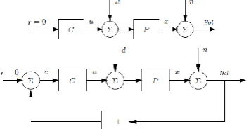
Let the disturbance is subjected to open loop and closed loop system as shown in Figure 4.

Tracking the signal for the loop shown in Figure 4, the exponential signal with output is

) ( ) ( ) ( ) ( 1

1 )

( S s y t

s C s P t

ycl  _ ol

(27)

where, S(s) is the sensitivity function.

To follow references closely and to reject the output disturbances, the sensitivity function must have a small magnitude at low frequencies; hence, its magnitude is to be less than some specified gain L [23] at some specified frequency₁.

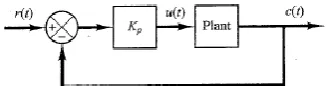
Figure 3. Closed loop system for proportional controller

TABLE 1.For critical gain and critical period

Type of controller Kp Ti Td

P 0.5 K_cr ∞ 0

PI 0.45 K_cr 1/1.2 P_cr 0

Figure 4. Open and closed loop systems subject to the same disturbances

L j

P j

C 

 ( ) ( ) 1

1

1

1 

 (28)

The robustness of the system occurs if the gain variation exists in the system and at the gain-crossover frequency the phase of the open-loop transfer function is to be (at least roughly) constant.

0 )]

( ) (

arg[ _ 

cg

jw P j C d

d

  

 (29)

8. EXAMPLES

Here we are conceding the general model [24] of DC motor as shown in Figure 5. The angular velocity (t)

is controlled by the applied voltage V_a.

The mathematically model of the DC Motor is given as in Figure 6. The obtained transfer function of the DC Motor is

] ) )( [( ) (

) ( ) (

m b f m

a DCM

K K K Js R Ls s

K s

V s s G

   

  (30)

In most application the time constant of DC Motor is negligible therefore the simplified continuous mathematical model has the following form:

Figure 5. General model of DC Motor

Figure 6. Mathematical model of a DC Motor

] ) ( [ ) (

) ( ) (

m b f

m

a DCM

K K K Js R s

K s

V s s G

    

) 1 (  

s KDCM

 

(31)

where,

) (

)

( _{f b m}

m DCM

m b

f RK K K

K andK

K K RK

RJ

  



 . It is

also note that K_m K_b

For the give DC Motor the physical parameter are as

 6 R

1 . 0



 b

m K

K

ms N Kf 0.2 

2 2

/ 01 .

0 kgm s J

With the help of given constant, obtained transfer function is

) 1 05 . 0 (

08 . 0 ) (

 

s s s

GDCM (32)

8.1. Controller Design by Ziegler-Nichols Method with Stability and Sensitivity Analysis The first requirement is to find out the starting point for K_p and

double zeros.

Let start the tuning with considering the K_p only. Here the closed loop response is:

P P ZN

K s s

K s

R s C Gcl

   

) 1 05 . 0 (

08 . 0 ) (

) (

(33)

By the help of Routh-Hurwitz criteria, the value ofK_P

for sustained oscillations is KP62.5

We set the value in MATLAB program with a hit and trial range. After putting the values in

) 1 1 ( )

( T s

s T K s

Gc d

i p

ZN    , we find out the controller

transfer function

s s s

s GcZN

1833 6 . 523 4 . 37 ) (

2_{ }



Therefore, here the initial values are obtained. As the requirement of industry, we can set the value of maximum overshoot in programming. Generally, according to the better establishment of the system, the overshoot should be between10% to 40%. Using the MATLAB program, we vary the gain 120 to 30 with step size -0.2 and zeros as 7 to 0.3 with step size -0.2. Fine tuning gives the following results

Gain (K) = 37.4and Zeros (a) = 7 Maximum overshoot (m) =1.05

The final close-loop transfer function of the system is:

6 . 146 89 . 41 992 . 3 05 . 0

6 . 146 89 . 41 992 . 2 ) (

2 3

2

  

  

s s

s

s s

s

GclZN (34)

2 3 2

05 . 0

6 . 146 89 . 41 992 . 2 ) (

s s

s s

s G_sol

  

 (35)

2 3 4 5 6

2 3 4 5

3 . 293 44 . 98 17 . 11 3992 . 0 0025 . 0

6 . 146 22 . 49 086 . 5 1496 . 0 ) (

s s s s s

s s s s s

Gscl

   

  

 (36)

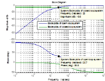
Figure 7 shows the stability region and Figure 8 Shows the step response of the system. The Bode plot of open loop and closed loop system is shown in Figure 9. Here the designed controller is by Ziegler-Nichols Method. The specification of gain crossover frequency and phase margin are obtained. The phase of the given system is forced to be flat at _cg and hence to be almost constant

within an interval around_cg.

8. 2. Stability Check and Robust Controller Design by Fractional-Order Method A robust controller is less sensitive to the parameter changes of the controlled system [25]. The uncertainty can be caused by non-precise identification. The fractional order controllers are less sensitive to changes of controlled system parameters.

The FOPDT system with parametric uncertainty can be represented as:

) 1 ] , ([

] , [ ) (



 _

 



s s

k k s G

 

(37)

where,k,and

 ,

k are the upper and lower limits of the given parameters.

Figure 7. Pole location on Pole-Zero Map of GclZN(s)

Figure 8. Unit step response of the closed loop GclZN(s) system

Figure 9. Bode plots of open loop Gsol(s) and closed loop Gscl(s) system

For maximum and minimum gain plot, the given system transfer function are shown respectively as:

) 1 ] ([

] [ ) (

1  _

 

s s

k s

GR _ (38)

) 1 ] ([

] [ ) (

2

  _

s s

k s G_R

 (39)

Consider the transfer function model of plant in given example is:

) 1 05 . 0 (

08 . 0

 

s s

GPlant (40)

We are using here the technique proposed in section 4 for fraction order controller design. According to this Step 1: - To design the KP

For minimum static error the value of proportional gain KP=10, from Equation (40)

Step 2: - Design of KD, μ, KI and λ

The value of a time constant τ = 0.05 and gain of Plant KPlant = 0.08 respectively Equation (40).

If we fix to gain margin ϕm>= 600

for the given control system. Then we find out the value of v = 0.3 by Equation(21). The other desired value k1 = 12.5 and k2 = 0.05 obtained from Equation (20). Now putting these values in Equation (22), we got

Now add the value of KP = 10 from step 1into Equation (41), we got final transfer function of fractional order controller as:

To make robust of the system an obtained controller transfer function is used with the transfer function

3 . 0 7 . 0 12.5 625

. 0 ) (

s s s

CFO   (41)

3 . 0 7 . 0 12.5 625

. 0 10 ) (

s s s

obtained for maximum and minimum gain as given in Equations (38) and (39).The open loop control system for controller and plant GR1(s) is:

3 . 1 3 . 2

3 . 0

1

04 . 0

25 . 1 0625

. 0 ) (

s s

s s s

GR_ol

  

 (43)

The close-loop transfer function of given control system with unity feedback is obtained as:

) ( ) ( 1

) ( ) ( ) (

1

s G s C

s G s C s G

Plant Plant cl

R  _

or

25 . 1 0625

. 0 04

. 0

25 . 1 0625

. 0 )

(

3 . 0 3

. 1 3 . 2

3 . 0

1

  



  

s s s

s

s s s

GR_cl (44)

The open loop control system for controller and plant GR2(s) is:

3 . 1 3 . 2

3 . 0

2

06 . 0

750 . 0 03750 . 0 6 . 0 ) (

s s

s s

s GR _ol

  

 (45)

The close-loop transfer function of given control system with unity feedback is obtained as:

750 . 0 6 . 0 03750 . 0 06

. 0

750 . 0 6 . 0 3750 . 0 )

(

3 . 0 3

. 1 3 . 2

3 . 0

2

  



  

s s s

s

s s s

GR _cl (46)

The function is stable checked the denominator of GR1cl(s) and GR2cl(s), it is found that K=1, indicate the system is stable. Here Figures 10 and 11 shows that system controlled by fractional order controller has more stability region. Figure 12 Indicate that the complete designed system is stable. The closed loop response of the system for both plants is almost same. This means that due to the parameter variation there is no such effect on the stability and system has a robust performance as shown in Figure 13.

9. CONCLUSIONS

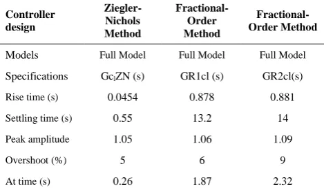
On behalf of the result shown in Table 2, some important point may be described for tuning of the controller.

Figure 10. Pole position of a closed loop system GR1cl(s)

Figure 11. Pole position of a closed loop system GR2cl(s)

Figure 12. Step response of closed loop system GR1cl(s) and GR2cl(s)

Figure 13. Simultaneously unit step response of all designed systems

All basic ideas of fractional calculus, the stability of fractional order system, sensitivity, robustness and MATLAB function are presented here. The robustness and sensitivity analysis is investigated for the given real-time example. The main purpose of the paper is to draw attention to fractional order system stability and analysis over a conventional way. Here an integer order plant is controlled by full order controller and fractional order controller. It concludes here that the fractional order system has robustness and a large region for

-1.5 -1 -0.5 0 0.5 1 1.5 -1.5

-1 -0.5 0 0.5 1 1.5

Pole-Zero Map

Real Axis

Im

a

g

in

a

ry

A

x

is

stable region

unstable region

-1.5 -1 -0.5 0 0.5 1 1.5 -1.5

-1 -0.5 0 0.5 1 1.5

Pole-Zero Map

Real Axis

Im

a

g

in

a

ry

A

x

is

unstable region stable region

0 5 10 15

0 0.2 0.4 0.6 0.8 1 1.2 1.4

time(sec)

O

u

tp

u

t

unit step response

GR1cl(s) Gr2cl(s)

Unit-Step Response

t Sec (sec)

O

u

tp

u

t

0 5 10 15

0 0.2 0.4 0.6 0.8 1 1.2 1.4

stability which improves the performance of the system. In Table 2 all transient parameter of fractional order controller design system and conventional controller design are given. The conventional controller design has a better transient response over fractional order controller design system. But in the fractional order, the larger stability region provides more flexibility in the system. We believe that the comparative approach used in this paper is useful for selecting the method of controller design.

TABLE 2. Comparison for performance specification of designed controllers

Controller design

Ziegler-Nichols Method

Fractional-Order Method

Fractional-Order Method

Models Full Model Full Model Full Model

Specifications GclZN (s) GR1cl (s) GR2cl(s)

Rise time (s) 0.0454 0.878 0.881

Settling time (s) 0.55 13.2 14

Peak amplitude 1.05 1.06 1.09

Overshoot (%) 5 6 9

At time (s) 0.26 1.87 2.32

10. REFERENCES

1. Gutman, P., Mannerfelt, C. and Molander, P., "Contributions to the model reduction problem", IEEE Transactions on

Automatic Control, Vol. 27, No. 2, (1982), 454-455.

2. Bandyopadhyay, B., Rao, A. and Singh, H., "On pade approximation for multivariable systems", IEEE Transactions

on Circuits and Systems, Vol. 36, No. 4, (1989), 638-639.

3. Smamash, Y., "Truncation method of reduction: A viable alternative", Electronics letters, Vol. 17, No. 2, (1981), 97-99. 4. Jamshidi, M., "An overview on the aggregation of large-scale

systems", IFAC Proceedings Volumes, Vol. 14, No. 2, (1981), 1309-1314.

5. Shamash, Y., "Model reduction using the routh stability criterion and the pade approximation technique", International Journal

of Control, Vol. 21, No. 3, (1975), 475-484.

6. Shahri, E.S.A., Alfi, A. and Machado, J.T., "Stabilization of fractional-order systems subject to saturation element using fractional dynamic output feedback sliding mode control",

Journal of Computational and Nonlinear Dynamics, Vol. 12,

No. 3, (2017), 0310141-0310146.

7. Alfi, A., Khosravi, A. and Lari, A., "Swarm-based structure-specified controller design for bilateral transparent teleoperation systems via μ synthesis", IMA Journal of Mathematical control

and Information, Vol. 31, No. 1, (2013), 111-136.

8. Mousavi, Y. and Alfi, A., "A memetic algorithm applied to trajectory control by tuning of fractional order proportional-integral-derivative controllers", Applied Soft Computing, Vol. 36, (2015), 599-617.

9. Alfi, A. and Fateh, M.-M., "Intelligent identification and control using improved fuzzy particle swarm optimization", Expert

Systems with Applications, Vol. 38, No. 10, (2011),

12312-12317.

10. Axtell, M. and Bise, M.E., "Fractional calculus application in control systems", in Aerospace and Electronics Conference, 1990. NAECON 1990., Proceedings of the IEEE 1990 National, IEEE., (1990), 563-566.

11. Dorcak, L., "Numberical models for simulation the fractional order control systems [j/ol]. Uefsav, the academy of science institute of experimental physcics, kosice, slovak republic, 1994 [2009-12-19]", arXiv preprint math/0204108, 62–68.

12. Hassanpour, H. and ROSTAMI, G.A., "Image enhancement via reducing impairment effects on image components",

International Journal of Engineering-Transactions B:

Applications, Vol. 26, No. 11, (2013), 1267-1274.

13. Soltani, J., Abjadi, N. and PAHLAVANI, N.M., "An adaptive nonlinear controller for speed sensorless PMSM taking the iron loss resistance into account (research note)", International

Journal of Engineering-Transactions B: Applications, Vol. 21,

No. 2, (2008), 151-160.

14. Oldham, K. and Spanier, J., "The fractional calculus theory and applications of differentiation and integration to arbitrary order, Elsevier, Vol. 111, (1974), ISBN: 9780080956206

15. Podlubny, I., "Fractional differential equations: An introduction to fractional derivatives, fractional differential equations, to methods of their solution and some of their applications, Elsevier, Vol. 198, (1998).

16. Miller, K.S. and Ross, B., "An introduction to the fractional calculus and fractional differential equations", (1993). 17. Samko, S., Kilbas, A. and Marichev, O., "Fractional integrals

and derivatives and some of their applications", Science and

Technica, Vol. 1, (1987), ISBN: 2881248640 9782881248641

18. Moghanloo, D. and Ghasemi, R., "Observer based fuzzy terminal sliding mode controller design for a class of fractional order chaotic nonlinear systems", International Journal of

Engineering-Transactions B: Applications, Vol. 29, No. 11,

(2016), 1574-1581.

19. Pilla, R., Tummala, A. and Chintala, M., "Tuning of extended kalman filter using self-adaptive differential evolution algorithm for sensorless permanent magnet synchronous motor drive",

International Journal of Engineering-Transactions B:

Applications, Vol. 29, No. 11, (2016), 1565-1573.

20. Chen, Y., Petras, I. and Xue, D., "Fractional order control-a tutorial", in American Control Conference, 2009. ACC'09., IEEE., (2009), 1397-1411.

21. Bidan, P., "Commande diffusive d'une machine electrique: Une introduction", in ESAIM: Proceedings, EDP Sciences. Vol. 5, (1998), 55-68.

22. Vinagre, B.M., Podlubny, I., Dorcak, L. and Feliu, V., "On fractional pid controllers: A frequency domain approach", IFAC

Proceedings Volumes, Vol. 33, No. 4, (2000), 51-56.

23. Yan, Z., He, J., Li, Y., Li, K. and Song, C., "Realization of fractional order controllers by using multiple tuning-rules",

International Journal of Signal Processing, Image Processing

and Pattern Recognition, Vol. 6, No. 6, (2013), 119-128.

24. Tajbakhsh, H. and Balochian, S., "Robust fractional order pid control of a dc motor with parameter uncertainty structure", Int.

J. of Innovative Science, Engineering & Technology, Vol. 1,

No. 6, (2014), 223-229.

25. Yeroglu, C. and Tan, N., "Note on fractional-order proportional– integral–differential controller design", IET Control

Stability and Robust Performance Analysis of Fractional Order Controller over

Conventional Controller Design

P. Kumar, S. Kumar Chaudhary

Electrical Engineering Department, SunRise University, Alwar, Rajasthan, India

P A P E R I N F O

Paper history: Received 12May 2017

Received in revised form 15June 2017 Accepted 12October 2017

Keywords:

Fractional Order Controller Fractional Order Calculus Stability

Performance Analysis Function Under Class Ziegler-Nichols Method

ديكچ ه

.تسا هدش داهنشيپ رلرتنک یحارط یا هسیاقم شور هلاقم نیا رد زا یدراوم یحارط و زيلانا اب نيسدنهم و نادنمشناد

یارب یضایر یاه لدم شیاديپ و لماكت ماگ نيلوا رد هک دنوش یم هجاوم یعقاو تلاكشم لح

دروم یعقاو تلاكشم

یربراک عبات تاقتشم و عبات لارگتنا .تسارجا لباق همانرب و حرط کی دننامه یضایر یاه لدم .دريگ یم رارق هجوت جرد ليسنارفید تلاداعم طسوت لرتنک دراوم .دراد یكيمانید یاهمتسيس لرتنک رد یعيسو رد ار زج تاقتشم ای لااب تا

.دريگ یم رب ادیاپ هلحرم نیا رد

ق یسررب دروم متسيس هجرد و یر ر

هحفص و هدودحم ردرادیاپ هيحان .دريگ یم را

رارق یا هديجيپ یم

لک روطب .دهديم یریذپ فاطعنا متسيس هب یسدنهم لرتنک یريگراكی رد عيسو رادیاپ هيحان .دريگ ی

و لرتنک یحارط شور زا رگا .دوش یم هتفرگ راكب یبرجت ليلحت شور و یددع زيلانا لح قورط ازجا لرتنک هجرد

.دهد یم یرتهب جیاتن اهرتماراپ لرتنک سپس دوش هتفرگ راكب