Please cite this article as: E. Ezzatneshan, Implementation of D3Q19 Lattice Boltzmann Method with a Curved Wall Boundary Condition for Simulation of Practical Flow Problems, International Journal of Engineering (IJE), TRANSACTIONS C: Aspects Vol. 30, No. 9, (September 2017) 1381-1390
International Journal of Engineering
J o u r n a l H o m e p a g e : w w w . i j e . i rImplementation of D3Q19 Lattice Boltzmann Method with a Curved Wall Boundary
Condition for Simulation of Practical Flow Problems
E. Ezzatneshan*
Aerospace Engineering Group, Department of New Technologies Engineering, Shahid Beheshti University, Tehran, Iran P A P E R I N F O
Paper history:
Received 05 February 2017 Received in revised form 23 May 2017 Accepted 07 July 2017
Keywords:
Three-dimensional Lattice Boltzmann Method
Irregular Wall Boundary Condition Laminar Fluid Flows
Complex Geometries
A B S T R A C T
In this paper, implementation of an extended form of a no-slip wall boundary condition is presented for the three-dimensional (3-D) lattice Boltzmann method (LBM) for solving the incompressible fluid flows with complex geometries. The boundary condition is based on the off-lattice scheme with a polynomial interpolation which is used to reconstruct the curved or irregular wall boundary on the neighboring lattice nodes. This treatment improves the computational efficiency of the solution algorithm to handle complex geometries and provides much better accuracy comparing with the staircase approximation of bounce-back method. The efficiency and accuracy of the numerical approach presented are examined by computing the fluid flows around the geometries with curved or irregular walls. Three test cases considered herein for validating the present computations are the flow calculation around the NACA0012 wing section and through the two different porous media in various flow conditions. The study shows the present computational technique based on the implementation of the three-dimensional Lattice Boltzmann method with the employed curved wall boundary condition is robust and efficient for solving laminar flows with practical geometries and also accurate enough to predict the flow properties used for engineering designs.
doi: 10.5829/idosi.ije.2017.30.09c.11
NOMENCLATURE Greek Symbols
l
C Lift coefficient K Permeability tensor Dynamic viscosity
d
C Drag coefficient L Length Kinematic viscosity
s
c Lattice sound speed l Lagrangien polynomial coefficient Density
D Diameter N Number of lattice nodes Relaxation time
d Distance p Pressure Weighting coefficient
e Particle velocity vector Re Reynols number t Lattice time step
f Pre-collicion distribution function u Flow velocity vector x Lattice grid size
f Post-collicion distribution function x y z, , Coordinate directions Subscripts eq
f Equilibrium distribution function Possible direction for particle velocity
1. INTRODUCTION1
In the past two decades, the lattice Boltzmann method (LBM), because of its mesoscopic and kinetic nature, has become a promising numerically robust technique
*Corresponding Author’s Email: [email protected] (E. Ezzatneshan)
Navier-Stokes solvers. This method therefore has been successfully applied to a wide range of hydrodynamic problems even with complex physics [1-5].
The standard LBM is adopted to the uniform Cartesian grid for solving flow problems with straight wall boundaries. Thus, the standard LBM has a major restriction for implementation of curve boundary condition which greatly limits its application to simulate
engineering practical problems with complex
geometries. Various efforts have been put forward to improve the efficiency of the standard LBM for the complex boundary implementation along the curved boundaries. The immersed boundary method is a mostly used approach within the Navier-Stokes (N-S) equations to treat fluid flows involving complex wall boundary conditions. This convenient method is extended to the framework of LBM and employed to simulate flow problems with curved wall boundaries [6]. In the immersed boundary method, a local force computes the effect of the wall on the fluid which is added by a source term to the governing equation. The existing of the forcing term in the LBM with immersed boundary approach impacts the stability of the numerical solution and restricts to use small CFL numbers which causes high computational cost.
Another methodology performed to tackle the LBM for solving of complex geometry flows is employing the most common bounce-back method [7] which is widely used for applying the wall boundary condition. However, implementation of the classical bounce-back scheme for the curved walls suffers from a low resolution near the boundary, since the smooth wall is basically approximated by a staircase segments. This drawback leads the LBM to be a method with only first-order accuracy in space [8].
A family of boundary fitting methods has been proposed in the literature to improve accuracy of the bounce-back scheme for resolving the irregular wall boundary and implementation of the LBM for simulation of such flow problems with appropriate precision. In the boundary fitting methods, the lattice nodes inside the fluid domain are considered as ‘fluid nodes’ and nodes outside of the fluid domain are so-called ‘solid nodes’. Then, to implement no-slip boundary condition on the curved wall, an inter- or extrapolation approach is used at the neighboring solid nodes to define the unknown distribution of the particles at the boundary nodes by using the known populations coming from fluid nodes. With this aspect, Verberg and Ladd [9] have developed a sub-grid model for LBM with considering the volume fraction associated with each fluid nodes near the wall boundary. A grid-refinement scheme is proposed by Filippova and Hanel [10] and then the inter- and extrapolation schemes have effectively developed by Mei et al. [11] and Guo et al. [12]. Latt et al. [13] have proposed a very general formalism which can use both of interpolation and
extrapolation of the velocity at the boundary nodes. Verschaeve and Muller [14] have extended the Latt et al.’s approach to curved boundary conditions which is verified for two-dimensional LBM and a thorough verification of the three-dimensional case is still necessary. Note that using an appropriate interpolation or extrapolation scheme for implementation of the curved boundary conditions allows to preserve spatial second-order of accuracy of the LBM near the boundaries [12, 14].
In the present work, the approach proposed by Verschaeve and Muller is extended and applied for three-dimensional LBM to solve practical flow problems with complex geometries. Herein, the standard D3Q19 single relaxation time lattice Boltzmann method (SRT-LBM) is implemented with employing the extended off-lattice wall boundary condition for simulation of laminar fluid flows. The computational efficiency and accuracy of the curved wall boundary condition employed is investigated in comparison with the bounce-back treatment. The robustness and accuracy of the SRT-LBM applied are examined by solving incompressible fluid flow around a NACA0012 wing section and through the two different porous media geometries at various flow conditions.
The rest of the present paper is organized as follows: In Section 2, the D3Q19 SRT-lattice Boltzmann method is presented. In Section 3, the implementation of the curved wall boundary conditions with an interpolated off-lattice scheme is given. The numerical results obtained for the three flow problems are presented and discussed in Section 4 to examine the performance of the solution methodology. Finally, the some conclusions are made in Section 5.
2. GOVERNING EQUATION
The single relaxation time LB equation used with the collision term in the Bhatnagar-Gross-Krook (BGK) approximation can be expressed as:
1 ( eq)
f
f f f
t
e (1)
where, f t c x( , , ) is the particle (mass) distribution function, is the relaxation time parameter and e
denotes the microscopic velocity of particles. feq
defines the equilibrium distribution function through a Chapman-Enskog expansion procedure and can be expressed as:
2 2
2 4 2
9 ( ) 3 1 3
2 2
eq
f
c c c
u
e u e u
(2)
A three-dimensional cubic lattice model with nineteen particle velocity directions (D3Q19) is employed to discretize Equation (1) in the lattice configuration as:
1
( eq) , 0,1,...,18
f
f f f
t
e (3)
where, denotes the possible direction of the particle velocity. Figure 1 shows the D3Q19 discrete Boltzmann model employed with the discrete velocity e. In the D3Q19 LBM, the weight factors and particle
velocity e are given as:
0 1 6 7 18
1 1 1
, ,
3 18 36
(4)
0, 0, 0
0( 1, 0, 0), (0, 1, 0), (0, 0, 1) 1 6 ( 1, 1, 0), ( 1, 0, 1), (0, 1, 1) 7 18
c c c
c c c
e (5)
where, c x/ t is the lattice speed. x and t are the grid spacing and the time step size, respectively, which are assumed to be unity.
The macroscopic density and velocity u are defined based on the particle distribution function as:
,
f f
u
e (6)and the pressure is expressed by the state formula 2
s
pc , where csc/ 3 is the sound speed. The kinematic viscosity depends on the speed of sound and relaxation time by the following definition:
2
( 0.5)
s c
(7)
The lattice Boltzmann equation discretized in Equation (3) is usually solved by a streaming-collision approach in two steps. First, the particles collide on the lattice nodes, known as ‘collision step’:
1
( , ) ( , ) [ ( , ) eq( , )]
f t x f t x f t x f t x
(8)
Figure 1. The cubic D3Q19 lattice model and the microscopic velocities
Second, propagation of the particle distributions occurs according to their respective speed, known as ‘streaming step’:
( , ) ( , )
f t t xe f t x (9)
where, f( , )t x and f( , )t x denote the pre- and post-collision states of the distribution function, respectively.
3. BOUNDARY CONDITIONS
In this section, the implementation of curved wall boundary condition and inlet/outlet open boundary conditions are described for the lattice Boltzmann method employed.
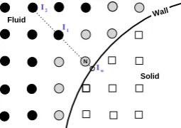
3. 1. Curved Wall Boundary Condition For implementation of general wall boundary conditions, the lattice nodes neighboring the curved wall is grouped into ‘fluid nodes’ inside the flow domain (F ), ‘boundary nodes’ near the wall (B) and ‘solid nodes’ outside of the flow domain (S ), which are shown in Figure 2 by the black circle, gray circle and square symbols, respectively. In this figure, the populations of
F , B and S for the boundary node N are
{6}, {0, 2,3,5, 7}, {1, 4,8}
F B S (10)
After streaming step, the populations streamed from nodes outside of the flow domain are unknown, e.g. for boundary node N they would be
2,3,6
. Herein, theunknown population on the boundary node N are considered as the opposite of solid node indices
{2,3,6}
opposite
S .
The macroscopic parameters and u are known after streaming on the fluid nodes and the no-slip boundary condition is imposed on the wall. On the boundary nodes however, the macroscopic flow
properties are unknown because of unknown
populations streamed in from the outside of flow domain. Because of the boundary node N is placed between the fluid nodes and the wall, the macroscopic quantities can be computed on the boundary nodes by an interpolation scheme.
Figure 2. Close view of the boundary node N and its neighbors
Wall
Solid Fluid
N
8 1 2
3
4 5 6
As shown in Figure 3, the velocity uN on the boundary node N of interest can be computed by interpolating the velocity between the fluid nodes I1, I2 and the wall
boundary condition at Iw. Herein, a quadratic Lagrangian interpolation scheme is employed as the following relation
N w wl 1 1l 2 2l
u u u u (11)
where, uw, u1 and u2 are the macroscopic velocity
vectors at the points Iw, I1 and I2, respectively. The coefficients of Lagrangian interpolation polynomial lw,
1
l and l2 are calculated as
1 2
1 2
N N
( )( )
,
I I
w
I I
d d d d
l
d d
(12)
2
1 1 2
N N
1
( )
,
( )
I
I I I
d d d
l
d d d
(13)
1
2 2 1
N N
2
( )
( )
I
I I I
d d d
l
d d d
(14)
where, d is the distance of the relevant node from the wall point Iw.
A local approximation algorithm is implemented to compute the density on the boundary node N as follows [14]:
N
post stream
pre collide f
g
KK
(15)
where, gpre collide geqgneq and K indicates the known populations on the boundary node N.
3. 2. Inlet/Outlet Boundary Conditions Each of inlet and outlet boundary conditions can be
implemented with Dirichlet- or Neumann-type
depending on the flow problem in question.
Figure 3. Approximating the macroscopic parameters at the boundary point N by an interpolating scheme
In the present work, the inlet and outlet boundary conditions for the porous media test cases are implemented using a Dirichlet-type to impose a constant pressure gradient along the geometry. The density is calculated by the state equation mentioned and the tangential velocity components are considered zero on the boundary nodes.
For simulation of flow around the NACA0012 wing section, all velocity components is imposed in the inlet (Dirichlet-type) and density is extrapolated from the interior domain. For the outflow, Neumann-type boundary condition is employed for the velocity to impose zero-gradient for this variable at the outlet boundary. A constant density is also considered by using the equation of state mentioned for a given pressure value in the outflow.
Finally, inlet/outlet boundary conditions should be defined for the distribution function f based on the known macroscopic variables on each boundary. Herein, the method proposed by Zou and He [15] is employed to evaluate the distribution function on the inlet and outlet boundaries.
4. RESULTS AND DISCUSSIONS
The accuracy and performance of the LBM
implemented are demonstrated by solving two flow problems with practical and complex geometries. Herein, the fluid flow around a NACA0012 wing section and flow through the two different porous media are considered at various flow conditions. The results obtained are compared with available data reported in the literature.
4. 1. Flow around the NACA0012 Wing Section
The aerodynamic surfaces (wing/blades) operate at low Reynolds numbers in a wide range of aerial applications, e.g. aircrafts in tack-off/landing situations, high-altitude long-endurance unmanned vehicles, micro-aerial vehicles and wind turbines. Flow treatment around the aerodynamic surfaces at low Reynolds numbers is different than high-Reynolds number condition due to strong adverse pressure gradients, laminar separation and reattachment of shear layers occur in downstream. These phenomena can impact aerodynamic efficiency of an aerial vehicle and have therefore led to different numerical and experimental studies for prediction of such low Reynolds number flow structures for improving practical designs.
The implemented LBM is used to simulate incompressible laminar flow around the NACA0012 wing section at Reu c0 /800 and 20 to examine the accuracy and efficiency of the present solution algorithm with comparing the results obtained with those of reported in the literature. Figure 4 shows the Wall
Solid Fluid
N
Iw
I1
cuboid flowfield with square cross section consists of the NACA0012 wing geometry. The spanwise and streamwise lengths of the domain are set to 40c and 10c, where c is the chord length of the NACA0012 airfoil. The wing is placed in distance of 5c from inflow boundary and located at the middle of cross section. Flow domain is also discretized by (1000 250 250) grid nodes.
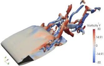
In Figure 5, the computed flowfield around the NACA0012 wing section is shown at middle plane in the spanwise direction of the wing by streamlines colored based on the velocity magnitude. Large separation bubbles due to relatively strong adverse pressure gradient on the suction side of the wing are obvious in this figure. The flow structure resolved indicates development of the von-Karman vortexes in the separated shear layer over the upper surface and shedding to the downstream. Figure 6 indicates a snapshot of the vertical vorticity magnitude iso-surface around the NACA0012 wing section. As can be seen in this figure, the laminar shear layer detaches in the von-Karman flow pattern lead to formation of curved vortex tubes in the spanwise direction with irregular shapes. In wing downwash, the vortices roll-up, interact together and create more complex three-dimensional structures.
Figure 4. The NACA0012 wing section at 20 in a cuboid computational domain
Figure 5. Computed flowfield for flow with Re800 around the NACA0012 wing section at 20 shown by streamlines in middle of the spanwise direction
Figure 6. Evaluated vertical component of the vorticity shown by iso-surface for flow with Re800 around the NACA0012
wing section at 20
The time averaged lift and drag coefficients computed using the present solution procedure for NACA0012 wing section at Re800 and 20 are compared with those of reported by Hoarau et al. [16] in Table 1. This comparison shows that the results obtained by the LBM implemented and those of obtained by Hoarau et al. are almost in good agreement and the small difference observed may be due to different numerical algorithms with different accuracies or different grid sizes/distribution applied. This study indicates that the LBM implemented with an appropriate curve wall boundary condition is efficient for simulation of laminar flow around the wing section used.
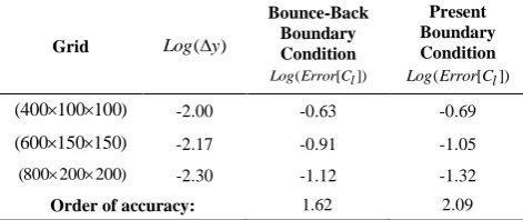
To demonstrate the efficiency and accuracy of the present boundary condition methodology for curved walls in comparison with the bounce-back treatment, the flow around the NACA0012 wing section is simulated by using three different grid sizes, namely, (400 100 100) , (600 150 150) and (800 200 200) to obtain the order of accuracy with employing these two boundary condition methods. The error is defined as the lift coefficient Cl difference for the three different meshes compared with the result of the most refined one, the mesh (1000 250 250) . The comparison results are given in Table 2. The results obtained show that the second order of accuracy of the solution is confirmed by employing the present boundary condition for this test case, while the accuracy of the solution obtained by implementing the bounce-back treatment is approximated 1.62.
TABLE 1. Comparison of the lift and drag coefficients for the NACA0012 wing section at Re800 and 20
Parameter Hoarau et al. (DNS) Present Solution (LBM)
l
C 0.94 0.983
d
C 0.43 0.386
X
0 200 400 600 800 1000
Y
0 100 200
Z
0 100
The error of the lift coefficient calculated based on the present boundary condition method for the flow around the NACA0012 wing section is also less than those of obtained based on the bounce-back treatment for the all grid sizes used in this study. It should be noted that the computational cost of the numerical solution with the both investigated boundary condition treatments is almost the same. This assessment indicates that the present solution methodology is satisfactorily accurate for simulation of the fluid flow around the practical geometries with curved wall boundary condition.
4. 2. Flow through the Porous Media
Understanding the fluid flow treatment in a porous medium is important for studying wide variety of applications in nature and industry. Transport phenomena of water in living plants and through the soil, oil recovery process, filtration and flow control in aerial vehicles are some of examples deal with the fluid flow in pore scales that show the crucial importance of studying such flow problems.
The pressure difference is responsible to drive the flow through porous medium by the viscous and inertial forces until a steady state condition reached. In the low pressure gradients, the viscous forces are dominant and the averaged flow velocity u can be determined by the Darcy’s law with the following linear equation:
K p
u (16)
where, K is the permeability tensor. The medium permeability K is a property depending on the size, distribution and connectivity of the pore spaces with constant values in each direction. Determination of this tensor for a particular porous medium needs numerous experiments, however easy to obtain by the computational techniques. For an imposed pressure gradient, the volume averaged velocity u can be calculated by the flow simulation through the medium and the permeability constant then would be obtained from Equation (16) if the flow be in Darcy regime. However, for high pressure gradients, the inertial forces between the fluid and porous surfaces dominate.
TABLE 2. Comparison of order of accuracy of the solution by employing two different wall boundary condition methods for simulation of flow around the NACA0012 wing section at
Re800 and 20
Grid Log(y)
Bounce-Back Boundary Condition
( [ l])
Log Error C
Present Boundary Condition
( [ l])
Log Error C
(400 100 100) -2.00 -0.63 -0.69
(600 150 150) -2.17 -0.91 -1.05
(800 200 200) -2.30 -1.12 -1.32
Order of accuracy: 1.62 2.09
In such conditions, the Darcy’s law is not valid anymore (non-Darcy regime) and the computational methods cannot be used for calculating the permeability tensor with the procedure mentioned. Therefore, properly understanding of the flow regimes is necessary in many applications to determine where the Darcy- and non-Darcy regimes occur and how much the critical pressure gradient is for a particular porous medium to flow switches from Darcy to non-Darcy regime.
The capability of LBM for simulation of fluid flow through the complex geometries suit this technique very well for modeling flow through the porous media [17-21]. In this section, the accuracy and performance of the present solution methodology implemented based on the LBM is demonstrated for simulation of fluid flow through the porous environment. Herein, two porous geometries are considered for flow computations to carry out the capability and robustness of the LBM presented for predicting those permeability properties. The critical pressure gradient in which the flow changes from Darcy to non-Darcy regime and the corresponding Reynolds number are also computed.
4. 2. 1. Porous Media with Regular Distribution of Spheres Figure 7 shows a slice extracted from a flow domain consists of a sphere in a body centered cubic. Mirrors of the slice in the x, y and z directions make a porous media with uniform distribution of spheres centered cubic. Due to similarity of the geometry in the all directions, the slice extracted can be chosen as the flow domain to reduce the computational cost. Physical diameter of the sphere and the length of the cube are Ds100m and L140m, respectively.
The present computations are performed with a (N Nx, y,Nz)(101,101,101) grid size for a wide variety of
pressure gradients, from p 106 to 1.5 10 1 in lattice unit, which are imposed in x direction. To calculate the medium permeability in different flow conditions, the variables of Darcy’s law in Equation (16) is converted to lattice units. Thus, the permeability tensor K can be defined in lattice unit as follows:
2
( )
& , ,
( )
s
i ij
D j
x u
K i j x y z
p N
(17)
where, 𝑁𝐷𝑆 denotes the number of lattice nodes discretized the length of sphere diameter in direction defined by the subscript j. Since the flow domain and porous geometry are periodic in the all directions for this test case, the 𝑁𝐷𝑆 value is constant, equals to
Figure 7. Regular sphere pack porous media with uniform distribution of spheres centered cubic
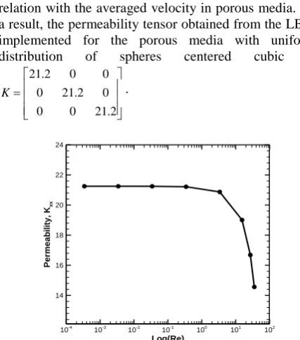
The results obtained for permeability by employing the present LBM is shown in Figure 8 for different pressure gradients applied in x direction. The horizontal axis of this figure defined by the Reynolds numbers calculated based on the average velocity in porous medium, after the steady state is reached for the attendant pressure gradient. The Reynolds number value is varied from
4
Re uDs 3 10
to 35 for p 106 to 1
1.5 10
used in present study. As can be seen in Figure 8, the medium permeability is constant Kxx21.2 for low
Reynolds numbers up to Re3.0, beyond which it decreases as Reynolds number increases. It means that the Darcy’s law is valid for the flow conditions up to Re3.0, where the flow regime transition to the non-Darcy flow is occurred at the pressure gradient
2 10
p
.
For lower p, the pressure gradient has a linear relation with the averaged velocity in porous media. As a result, the permeability tensor obtained from the LBM implemented for the porous media with uniform
distribution of spheres centered cubic is
21.2 0 0
0 21.2 0
0 0 21.2
K
.
Figure 8. Permeability of the porous media with uniform distribution of spheres centered cubic for different pressure gradients defined by the resultant Reynolds numbers
For verification of the accuracy of the permeability value computed by the present LBM, the result obtained is compared with that of the empirical relation proposed by Ergun [22]:
3 2
2
(1 )
s empirical
p
D K
A
(18)
where, Pore SpaceVolume
Bulk Volume
is porosity and Ap is a
geometric factor which is usually set to 175 180 . The permeability computed by Equation (18) for the porous media with uniform distribution of spheres is equal to
22.7
empirical
K which shows good agreement between
the empirical estimation and the computed results by the LBM implemented. Note that the porosity of the medium shown in Figure 7 is calculated after discretization of the flow domain with (101)3 lattice
nodes and it is equal to 54.58%. The permeability value computed can be converted from lattice unit to the physical unit by the scale conversion factor as follows
11 2
4.08 10
physical LBM
x L
K K m
N
(19)
In Figure 9, the computed flow fields are depicted by the streamlines colored based on the velocity magnitude
for p 105 and 1.5101.
Figure 9. Computed flowfield for the porous media with uniform distribution of spheres shown by streamlines and velocity magnitude with p 105, Re34104 (top) and
1
1.5 10
p
, Re35.3 (bottom)
Log(Re)
P
e
rm
e
a
b
il
it
y
,
Kx
x
10-4 10-3
10-2 10-1
100 101
102 14
This figure indicates that by increasing the pressure gradient imposed, the averaged flow velocity magnitude and consequently the Reynolds number increased. In such flow condition through the porous media, notably inertial effects are responsible for the additional pressure drop, known as the non-Darcy flow regime. This investigation shows that the lattice Boltzmann method employed is appropriate for accurate simulation of fluid flow through the porous media.
4. 2. 2. Porous Media with Irregular Distribution of Merged Spheres To demonstrate the accuracy and robustness of the LBM implemented for numerical solution of the flow problems with more complex geometries, the flow through a porous medium with irregular geometry is performed. The porous media shown in Figure 10, consists of a tight distribution of spheres in a cuboid pack that some of them merged
together. The dimension of the cuboid are
(L L Lx, y, z)(640,720,630)m, in which discretized by
(Nx,Ny,Nz)(301,338, 296) lattice nodes. According to
the numerical computations performed for the previous
test case, the pressure gradient is set p 105 for the present porous media to be sure about Darcy flow regime through the medium.
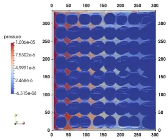
Figure 11 indicates the flowfield simulated by the present solution algorithm with the streamlines colored based on the velocity magnitude. For this test case, due to the microscopic pore size and complexity of the geometry, the fluid flow path is very tortuous and twisted. In addition, the complex nature of the solid-pore interface impacts the pressure distribution through the porous media. Thus, it is necessary to have pressure drop estimation along the porous media in many applications. It helps to study the productivity of the medium used and replace/design an appropriate geometry if needed. Herein, the computed pressure distribution field is shown at slice Nz100 through the porous media in Figure 12. A significant pressure drop along the porous media is obvious in this figure.
Figure 10. Irregular sphere pack porous media with a tight distribution of merged spheres
Figure 11. Computed flowfield for the porous media with irregular distribution of spheres shown by streamlines and
velocity magnitude with p 105 applied in x direction
Figure 12. Computed flowfield of the porous media with irregular distribution of spheres with 5
10
p
shown by streamlines and pressure distribution in the xy plane at
100
z
N
To compute the permeability tensor for the porous media shown in Figure 10 by employing the LBM implemented, the pressure gradient p 105 is imposed in three directions x, y and z. The results obtained for the permeability of the porous media with irregular distribution of merged spheres is presented in Table 3. The physical permeability tensor is again calculated according to Equation (19). This study shows the capability of the present numerical solution technique based on the LBM for simulation of the flow problems with irregular and complex geometries.
TABLE 3. Permeability properties of the irregular sphere pack porous media
Direction KLBM KPhysical(m2)
x 2.075 9.41×10⁻¹²
y 2.482 1.13×10⁻¹¹
5. CONCLUSION
In this work, a 3-D lattice Boltzmann method is implemented for numerical simulation of flow problems with complex geometries. An off-lattice type wall boundary condition with appropriate Lagrangian polynomial interpolation is used to resolve the flow properties near the curved or irregular wall boundaries. It is shown that such a procedure can accurately resolve the flow field near the curved wall boundaries compared to the bounce-back treatment. The efficiency and accuracy of the numerical approach presented are examined by computing the incompressible laminar flow around the NACA0012 wing section and flow through the two different porous media with regular and irregular geometries. The calculations are performed for different laminar flow conditions and the results are compared with available data reported in the literature for the test cases considered. Validation results show good comparison for flow properties between LBM simulation and the empirical estimation and numerical results. The present study shows the computational technique based on the implementation of the three-dimensional Lattice Boltzmann method with the employed curved wall boundary condition. It is robust and efficient for solving flow problems with realistic and practical geometries and accurate enough to predict the flow properties used for engineering designs.
6. ACKNOWLEDGMENTS
The author would like to thank Shahid Beheshti University for the support of this research.
7. REFERENCES
1. Chen, S., Chen, H., Martnez, D. and Matthaeus, W., "Lattice boltzmann model for simulation of magnetohydrodynamics",
Physical Review Letters, Vol. 67, No. 27, (1991), 3776.
2. Premnath, K.N. and Abraham, J., "Three-dimensional multi-relaxation time (mrt) lattice-boltzmann models for multiphase flow", Journal of Computational Physics, Vol. 224, No. 2, (2007), 539-559.
3. Chakraborty, S. and Chatterjee, D., "An enthalpy-based hybrid lattice-boltzmann method for modelling solid–liquid phase transition in the presence of convective transport", Journal of
Fluid Mechanics, Vol. 592, (2007), 155-175.
4. Ashorynejad, H., Sheikholeslami, M. and Fattahi, E., "Lattice boltzmann simulation of nanofluids natural convection heat transfer in concentric annulus", International Journal of
Engineering-Transactions B: Applications, Vol. 26, No. 8,
(2013), 895-402.
5. Luo, K., Yao, F.-J., Yi, H.-L. and Tan, H.-P., "Lattice boltzmann simulation of convection melting in complex heat storage
systems filled with phase change materials", Applied Thermal
Engineering, Vol. 86, (2015), 238-250.
6. Shu, C., Liu, N. and Chew, Y.-T., "A novel immersed boundary velocity correction–lattice boltzmann method and its application to simulate flow past a circular cylinder", Journal of
Computational Physics, Vol. 226, No. 2, (2007), 1607-1622.
7. Ziegler, D.P., "Boundary conditions for lattice boltzmann simulations", Journal of Statistical Physics, Vol. 71, No. 5, (1993), 1171-1177.
8. Ginzbourg, I. and Adler, P., "Boundary flow condition analysis for the three-dimensional lattice boltzmann model", Journal de
Physique II, Vol. 4, No. 2, (1994), 191-214.
9. Verberg, R. and Ladd, A., "Lattice-boltzmann model with sub-grid-scale boundary conditions", Physical Review Letters, Vol. 84, No. 10, (2000), 2148-2154.
10. Filippova, O. and Hänel, D., "Boundary-fitting and local grid refinement for lattice-bgk models", International Journal of
Modern Physics C, Vol. 9, No. 08, (1998), 1271-1279.
11. Mei, R., Luo, L.-S. and Shyy, W., "An accurate curved boundary treatment in the lattice boltzmann method", Journal of
Computational Physics, Vol. 155, No. 2, (1999), 307-330.
12. Guo, Z., Zheng, C. and Shi, B., "An extrapolation method for boundary conditions in lattice boltzmann method", Physics of
Fluids, Vol. 14, No. 6, (2002), 2007-2010.
13. Latt, J., Chopard, B., Malaspinas, O., Deville, M. and Michler, A., "Straight velocity boundaries in the lattice boltzmann method", Physical Review E, Vol. 77, No. 5, (2008), 056703.
14. Verschaeve, J.C. and Müller, B., "A curved no-slip boundary condition for the lattice boltzmann method", Journal of
Computational Physics, Vol. 229, No. 19, (2010), 6781-6803.
15. Zou, Q. and He, X., "On pressure and velocity boundary conditions for the lattice boltzmann bgk model", Physics of
Fluids, Vol. 9, No. 6, (1997), 1591-1598.
16. HOARAU, Y., BRAZA, M., Ventikos, Y., Faghani, D. and Tzabiras, G., "Organized modes and the three-dimensional transition to turbulence in the incompressible flow around a NACA0012 wing", Journal of Fluid Mechanics, Vol. 496, (2003), 63-72.
17. Boek, E.S., Chin, J. and Coveney, P.V., "Lattice boltzmann simulation of the flow of non-newtonian fluids in porous media",
International Journal of Modern Physics B, Vol. 17, (2003),
99-102.
18. Sullivan, S., Gladden, L. and Johns, M., "Simulation of power-law fluid flow through porous media using lattice boltzmann techniques", Journal of Non-Newtonian Fluid Mechanics, Vol. 133, No. 2, (2006), 91-98.
19. Javaran, E.J., Nassab, S.G. and Jafari, S., "Numerical simulation of a three-layered radiant porous heat exchanger including lattice boltzmann simulation of fluid flow", International Journal of
Engineering-Transactions A: Basics, Vol. 24, No. 3, (2011),
301-319.
20. Fattahi, E., Waluga, C., Wohlmuth, B., Rüde, U., Manhart, M. and Helmig, R., "Lattice boltzmann methods in porous media simulations: From laminar to turbulent flow", Computers &
Fluids, Vol. 140, (2016), 247-259.
21. Wu, Z.-S., Dong, P.-C., Lei, G., Yang, S. and Cao, N., "Lattice boltzmann simulation of fluid flow in complex porous media based on ct image", Journal of Industrial and Intelligent
Information Vol, Vol. 4, No. 1, (2016).
22. Ergun, S., "Fluid flow through packed columns", Chemical
Implementation of D3Q19 Lattice Boltzmann Method with a Curved Wall Boundary
Condition for Simulation of Practical Flow Problems
E. Ezzatneshan
Aerospace Engineering Group, Department of New Technologies Engineering, Shahid Beheshti University, Tehran, Iran P A P E R I N F O
Paper history:
Received 05 February 2017 Received in revised form 23 May 2017 Accepted 07 July 2017
Keywords:
Three-dimensional Lattice Boltzmann Method
Irregular Wall Boundary Condition Laminar Fluid Flows
Complex Geometries
ديكچ ه
میمعت هراوید یزرم طرش عون کی ،رضاح هلاقم رد هس نمزتلوب هکبش شور یارب هتفای
شیازفا ببس هک هدش لامعا یدعب
رد نآ تقد و یدنمناوت هیبش
نایرج یزاس مکارت یاه
هسدنه لوح ریذپان یم هدیچیپ یاه
متیروگلا کی زا شور نیا .دوش
نورد هلمجدنچ یبای نایم و هاوخلد ینحنم هراوید لحم نیمخت تهج یا
یم هدافتسا هراوید فارطا هکبش طاقن یور نآ یبای
-شور هب تبسن ار نآ تقد و یددع لح -شور ییآراک متیروگلا نیا .دنک اه
موسرم ی
Bounce-Back
نایرج لح یارب
هسدنه لوح یم شیازفا هدیچیپ یاه
ناشن یارب .دهد هکبش شور ساسا رب هدافتسا دروم متیروگلا تقد و تحص نداد
هس نمزتلوب لوح نایرج ،یدعب لیوفوردیه عطقم اب لاب کی
NACA0012
زا هدنرذگ نایرج و ود
لخلختم طیحم ازجم
ررب دروم فلتخم طیارش رد هدش یبایزرا و هسیاقم سرتسد لباق جیاتن اب لصاح جیاتن و هتفرگ رارق یس
تسا . جیاتن هب
تسد هدمآ زا لح رضاح ناشن یم دنهد هک تیروگلا هداد هعسوت م نایرج لیلحت تهج ،نمزتلوب هکبش شور ساسارب هدش
یاه مکارت ریذپان هسدنه اب یدربراک و هدیچیپ یاه تاصخشم نیمخت یارب نینچمه
یحارط رد هدافتسا تهج نایرج یاه