A Collocation Method with Modified Equilibrium on Line Method for Imposition of Neumann and Robin Boundary Conditions in Acoustics (TECHNICAL NOTE)

TECHNICAL NOTE

A COLLOCATION METHOD WITH MODIFIED EQUILIBRIUM

ON LINE METHOD FOR IMPOSITION OF NEUMANN AND

ROBIN BOUNDARY CONDITIONS IN ACOUSTICS

A. Sadeghirad*, I. Mahmoudzadeh Kani and A. Vaziri Astaneh Department of Civil Engineering, University of Tehran

P.O. Box 11365-4563, Tehran, Iran

[email protected] – [email protected] – [email protected]

*Corresponding Author

(Received: March 9, 2009 – Accepted in Revised Form: November 5, 2009)

Abstract A collocation method with the modified equilibrium on line method (ELM) for imposition of Neumann and Robin boundary conditions is presented for solving the two-dimensional acoustical problems. In the modified ELM, the governing equations are integrated over the lines on the Neumann (Robin) boundary instead of the Neumann (Robin) boundary condition equations. In other words, integration domains are straight lines for nodes located on the Neumann boundary. Numerical examples of two-dimensional acoustical problems are presented to demonstrate the stability, accuracy and convergence of the proposed method.

Keywords Acoustics, Helmholtz Equation, Meshless Methods, Collocation Methods, Modified Equilibrium on Line Method (MELM), Moving Least Squares (MLS), Radial Basis Functions (RBF)

هﺪﻴﻜﭼ

يﺎﺿرارﻮﻈﻨﻣﻪﺑ

ﺖﺳا هﺪﺷ ﻪﺋارا يﺪﻌﺑ ود ﻚﻴﺘﺳﻮﻛآ ﻞﻳﺎﺴﻣ ﻞﺣ ياﺮﺑ ﻦﻴﺑار و ﻦﻣﻮﻴﻧيزﺮﻣ ﻂﻳاﺮﺷ

.

ﻂﺧ ﺮﺑ لدﺎﻌﺗ شور رد

ﻂﺧهرﺎﭘﺮﺑلدﺎﻌﺗ،هﺪﺷحﻼﺻا ﻦﻣﻮﻴﻧزﺮﻣيﺎﻫ

)

ﻦﻴﺑار

(

يزﺮﻣطﺮﺷ تﻻدﺎﻌﻣناﻮﻨﻋﻪﺑ

ﻲﻣﺎﺿراﻦﻣﻮﻴﻧ دﻮﺷ

.

ﻪﺑ

هﺮﮔياﺮﺑﻢﻴﻘﺘﺴﻣيﺎﻫﻂﺧهرﺎﭘ ﺮﮕﻳدنﺎﻴﺑ لاﺮﮕﺘﻧاﻲﺣاﻮﻧﻦﻣﻮﻴﻧزﺮﻣﺮﺑ ﻊﻗاويﺎﻫ

ﻲﻣﻞﻴﻜﺸﺗ اريﺮﻴﮔ ﺪﻨﻫد

.

ﻪﺑ

ﺖﺳاهﺪﻳدﺮﮔﻞﻴﻠﺤﺗيدﺪﻋلﺎﺜﻣﺪﻨﭼيﺪﻌﺑودﻚﻴﺘﺳﻮﻛآﻚﻴﻧﻮﻣرﺎﻫﻞﻴﻠﺤﺗردشورﻦﻳايﺎﻳاﺰﻣﻲﺳرﺮﺑرﻮﻈﻨﻣ رﻲﻳاﺮﮕﻤﻫوﺖﻗد،يراﺪﻳﺎﭘهﺪﻣآﺖﺳﺪﺑﺞﻳﺎﺘﻧو ﻲﻣنﺎﺸﻧاررﻮﻛﺬﻣشو

ﺪﻫد

.

1. INTRODUCTION

The Helmholtz equation is a linear mathematical model that describes time-harmonic acoustics, elastic and electromagnetic steady state waves. Analytical solutions to these problems are used only in relatively few cases. Therefore, numerical techniques such as finite element and boundary element methods are widely used in these analyses. In recent years, meshless methods have been developed and used to solve partial differential equations. Comprehensive reviews of meshless methods can be found in the literature [1-3]. These methods also have been applied for solving Helmholtz equation, such as [4-7].

The attractive advantage of the collocation-based meshless methods is that they are simple to

Sadeghirad, et al [13] proposed a modified version of the ELM. In the modified ELM, for any node located on the Neumann (or Robin) boundary, weak formulation of the governing equations is satisfied on two lines that connect the node in question to the two neighboring nodes on Neumann (or Robin) boundary.

In this paper, a collocation method with the modified ELM is applied to solve the two-dimensional acoustical problems. The performance of the modified ELM is studied for collocation methods based on two different schemes to construct meshless shape functions: moving least squares (MLS) approximation and locally supported radial basis point interpolation (RPIM). Two numerical examples of two-dimensional acoustics are presented to demonstrate the stability, accuracy and convergence of the proposed method.

2. MESHLESS SHAPE FUNCTIONS CONSTRUCTION SCHEMES

A number of ways to construct shape functions have been proposed. In this section, a brief description of the MLS and RPIM is given below.

2.1. Moving Least Squares (MLS)

Approximation

 (1)

Where p(x) is a vector of basis monomials and





aT  1 2 m is a vector of

coefficients; where m is the number of basis monomials. a(x) is obtained at any point x by

minimizing a weighted, discrete L2 norm as

follows:

2 n

1

i (xi)a(xi)

T p i u ) i x x ( w 2 n 1

i (xi)

h u i u ) i x x ( w J                   (2)

Where n is the number of nodes in the neighborhood of point x for which the weight function w(xx_i)0. u_i is the nodal value parameter of u at xxi, while uh(xi) is the

approximate value.

Using the stationarity condition for J in Equation 2 with respect to a(x), we can solve for a(x). By substituting it into Equation 1, the final approximation is obtained as follows:

    n

1 i i(x)ui )

x ( h

u (3)

Where the MLS shape function _i(x) is defined by:           m 1

j (x)B(x) ji

1 A ) x ( j p

i (4)

Where A(x) and B(x) are the matrices defined by:

) i x (x w (x) i w , n 1

i (xi)

T )p i (x)p(x i w A(x)      (5) )] n x ( p ) x ( n w , ), 2 x ( p ) x ( 2 w ), 1 x ( p ) x ( 1 w [ B(x)   (6)

A Gaussian weight function with the compact support property is adopted in the present work. The weight function corresponding to node i may be written as:

                                         i m r ir , 0 i m r ir 0 , 2 i c / i m r e 1 2 i c / i m r e 2 i c / i r e ) i r ( i w (7) Where r_i  xx_i is the distance from node x_i to

point x, c_i is a constant controlling the shape of the weight function w_i and r_mi is the size of the support domain.

the nodal values, i.e. the MLS shape functions given by Equation 4 do not, in general, satisfy the Kronecker delta condition.

2.2. Radial Basis Point Interpolation

Method (RPIM)

(x)

u , using RPIM, can be written as [15]:

      m 1 j j )b x ( j p n 1 i i (r)a i R ) x ( h

u (8)

With the constraint condition

m ,..., 2 , 1 j n 1 i , 0 i )a i x ( j p  

  (9)

Where R_i(r) is the radial basis function (RBF), r is the distance between the interpolation point x and node x_i, n is the number of nodes in the neighborhood of x, p_j(x) is the basis monomials, m is the number of basis monomials, scalar coefficients a_i and b_j are interpolation constants. By satisfying Equation 8 at the n nodes surrounding point x, Equations 8 and 9 can be rewritten in matrix form as follows:

                   b a 0 T P P R 0 u (10)

Where u













b _ are the vectors of the interpolation constants, R and P are defined as follows:

m n ) n x ( m p ) n x ( 1 p ) 1 x ( m p ) 1 x ( 1 p P , n n ) n r ( n R ) n r ( 1 R ) 1 r ( n R ) 1 r ( 1 R R                                 (11)

The coefficients a_i and b_j can be solved by using the following algorithm: From Equation 8, a can be solved, Pb 1 R u 1 R

a    (12)

Substituting Equation 12 into Equation 9 gives:

1 R T P 1 ) P 1 R T P ( b S , u b S

b     (13)

Also, substituting Equation 13 back into Equation 12 gives: ) b PS n n I ( 1 R a S , u a S

a   _  (14)

Where I_n_n is the identity matrix. By substituting

Equations 13 and 14 into Equation 8, the final approximation is obtained as follows:

u ) x ( Φ ) x ( h

u  (15)

Where the RPIM shape function Φ(x) is defined by: b S ) x ( T p a S ) x ( T R )] x ( n , ), x ( 2 ), x ( 1 [ ) x ( Φ       _ (16)

There are a number of forms of radial basis functions used by the mathematics community. In this paper the following multiquadrics (MQ) radial basis is applied.

q ) 2 C 2 ir ( (r) i

R   (17)

There are two parameters (C and q) that influence the performance of RPIM using the MQ radial basis function. C is the characteristic length related to the nodal spacing in the support domain of the interpolation point x.

It can be deduced from the above discussion that the RPIM passes through the nodal values, i.e. the RPIM shape functions given by Equation 16 satisfy the Kronecker delta condition.

3. DISCRETIZATION OF HELMHOLTZ EQUATION IN A COLLOCATION

METHOD

around a steady uniform state) is as follows:

 

   

   

 

in 2 t

p 2 2 c

1 2 y

p 2 2 x

p 2

(18)

Where p and c denote the field of acoustic pressure and speed of sound in the fluid, respectively.

We assume that the phenomena are steady harmonic, i.e.

) t j exp( p

p  (19)

Where ω is the angular frequency. By substituting Equation 19 into Equation 18 the spatial distribution p of the acoustic pressure (which is now a complex variable) can be obtained from Helmholtz equation as follows:

 

     

in 0 p 2 k 2 y

p 2 2 x

p 2

(20)

Where the wave number k is defined by the ratio between the angular frequency and the speed of sound:

c

k (21)

In order to completely address the acoustic problem, Helmholtz Equation 20 is associated with boundary conditions. Assume that problem domain

 enclosed by boundary _D_N_R with corresponding Dirichlet, Neumann and Robin boundary conditions as follows:

D on p

p  (22a)

N on n v ck j n p or n v n

v   

 

 (22b)

R on p n ckA j n p or p n A n

v   

 

 (22c)

Where , A_n and n are the specific mass of the fluid, the admittance coefficient modeling the damping and the unit outward vector to the boundary , respectively. Also, v is the particle velocity linked to the gradient of the acoustic

pressure through the equation of motion as follows:

0 p v ck

j   (23)

The discretized system of equations in a collocation method is formed by substituting the approximation (3 or 15) into Equations 20 and 22 and collocating the differential equation at each node in the analysis domain. Note that if RPIM shape functions are used in the collocation method, the Dirichlet boundary conditions can be imposed simply by substituting the prescribed pressures. In contrast, If MLS shape functions are used, the standard collocation method is applied to impose the Dirichlet boundary conditions because in contrary to the RPIM, the MLS approximation does not satisfy the Kronecker delta condition. This discretization leads to a system of algebraic equations of the form:

b

Kp (24)

Where K is the ‘stiffness’ matrix; b is the vector containing the prescribed values of the pressure and particle velocity on the boundaries; and p is a vector of unknown nodal pressures p_i. It can be easily seen that the stiffness matrix in the presented collocation method is banded because the support domains are compact. However, in general, K is asymmetric.

4. THE MODIFIED ELM FOR IMPOSITION OF NEUMANN (ROBIN) BOUNDARY

CONDITIONS

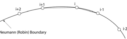
On Neumann and Robin boundaries, the derivatives of pressure exist in boundary condition equations. In the modified ELM, by integrating the governing differential Equation 20 over segments of the Neumann and Robin boundaries and a simple finite difference approximation, these derivatives of pressure emerge in the formulation. In contrary to direct imposition of Neumann boundary conditions, in the modified ELM, these boundary conditions are satisfied by a set of weak-form equations consistent with equations governing the body itself. Line ₁ connects two nodes i1

Figure 1. Hence for node i on the Neumann or Robin boundary, the governing differential Equation 20 in the global coordinate system is integrated over two lines *

1

 and * 2

 generated by slightly moving the lines ₁ and ₂ (Figure 2). In the modified ELM, two balanced areas (B-Areas) are defined for any node i on the Neumann boundary. These surfaces are constructed by dragging the lines ₁ and ₂ along the unit vector

*

n which is inward and orthogonal to line segment (Figure 2). The width of these surfaces is determined by the following equation:

s l s

 (25)

Where _s is the width of B-Area, l_s is the length of line _s and  is a user defined parameter. The local coordinate system (t*,n*) _{for these surfaces}

is defined as follows: its origin is located on node i; the orientation of local axis _t* _{is from node i to}

node i1 or i1; and the local system is a right-handed orthogonal system. Lines *

1

 and 2* are the

mid lines of these surfaces (Figure 2). Additionally it should be mentioned that curved boundaries are being treated by approximation with straight lines.

In the following, the formulation of the modified ELM is presented for the 2-D Helmholtz equation. By substituting Equation 23 into Equation 20, Helmholtz equation can be rewritten in the following form:

         in 0 p c k j y y v x x v (26)

Where v_x and v_y are the components of the particle velocity respect to the x and y directions, respectively.

In order to impose the Neumann (Robin) boundary conditions, Equation 26 should be integrated over two lines *

1

 and * 2

 for any node i on the Neumann (Robin) boundary. Lines *

1

 and * 2 

are the mid lines of two balanced areas (Figure 2),

0 2 1 s d *

s cp)w(rs)

k j y y v xx v (              (27)

Where w(r_s) is the test function and r_s is the

distance from node i along line _s. In the present work, the Gaussian test functions are used [13]:

4 s c s l , ] 2 s c / s l exp[ 1 ] 2 s c / s l exp[ ] 2 s c / s r exp[                         (28)

Where l_s is the length of line _s.

The derivatives appearing in Equation 26 can be rewritten with respect to the local coordinate system (t*,n*)_,

0 2

1

s d

*

s cp)w(rs)

k j * n * n v * t * t v (              (29)

The following finite difference approximations can be used so that the normal heat flux can appear in the formulation (Figure 2):

2 , 1 s , * * s * n v s * n v s s * s * n * n v                     (30) Figure 1. Determination of the integration domain of node xi

located on the Neumann boundary.

Figure 2. Balanced areas and their local coordinate systems

Where δs is the width of B-Area, and κs is defined as,

* n s n s 

 (31)

Where ns and n* are the unit outward vectors and

unit vector along local axis n* _{corresponding to}

line Гs, respectively (Figure 2). By substituting

Equations 22b, 23 and 30 into Equation 29 and rewriting the derivatives with respect to the global coordinate system (x,y), final formulation for satisfying the Neumann boundary conditions can be obtained as follows:

                                      2 1 s d s vnw s s ck j 2 1 s d * *

s )w

x s t y p y s t x p ( s s d w ) p 2 k 2 ) y s t ( 2 y p 2 2 1 s * s ) y s t )( x s t ( y x p 2 2 2 ) x s t ( 2 x p 2 ( (32)

Where x s

t and y s

t are the components of unit vector along the local axis t* corresponding to line Гs. The integrals in Equation 32 can be easily

evaluated over the straight lines via the Gauss quadrature technique.

In the similar way, the final formulation for satisfying the Robin boundary conditions can be obtained as follows:

0 2

1 s

d s Anpw s s ck j 2 1 s d * *

s )w

x s t y p y s t x p ( s s d w ) p 2 k 2 ) y s t ( 2 y p 2 ) y s t )( x s t ( y x p 2 2 2 1 s * s 2 ) x s t ( 2 x p 2 (                                       (33)

5. NUMERICAL EXAMPLES

Two numerical examples of two-dimensional

acoustics problems are considered to illustrate the performance of the collocation method with modified ELM in comparison to the direct collocation method. The size of the support domains (r_mi) is defined as,

i S j , i x j x max i c , i c i m

r     (34)

Where S_i is minimum set of neighboring nodes of

i

x which construct a polygon surrounding node

i

x ; and 3.5 is used in the computation. Also, the weight function in the MLS approximation is the Gaussian weight function (Equation 7) with

5 c r

i

mi  ; and in application of the MQ-RBF

(Equation 17), q2.05 is used, and C is defined as,

0 C

C (35)

Where C₀ is the average distance between all nodes in the support domain, and 1 is chosen. The ratio of width of the balanced area to its length in Equation 25 is chosen as 0.3. Also, Numerical integration is carried out using 5 Gauss points along any line. The second order basis functions (m6) are used in the MLS approximation (Equation 1) and the linear polynomial is added in the RPIM (Equation 8). The above values were chosen based on the results obtained on the previous work [13].

For the purpose of error estimation and convergence studies, the following error norm is adopted,       N 1 i 2 ) exact i u ( N 1 i 2 ) app i u exact i u (

Error (36)

Where exact i

u and app i

u are respectively the exact and approximate values of u_i and N is the total number of discrete values.

5.1. Closed Wave-Guide

the Neumann boundary conditions is studied for a standing plane wave within a 1 m × 1 m domain. This problem deals with the following boundary conditions:

m / Pa 0 ) 1 , x ( y p ) 0 , x ( y p

, Pa 0 ) y , 1 ( p , Pa 1 ) y , 0 ( p

    



 

(37)

The standing plane wave can be calculated analytically by:

) 1 k sin(

)] x 1 ( k sin[ ) y , x ( p

 

 (38)

The speed of sound in the media is assumed to be c = 300 m/s. The problem is solved for three different frequencies f1 = 500 Hz, f2 = 700 Hz and

f3 = 1000 Hz. The calculations are carried out

using four irregular nodal distributions, with 121, 441, 961 and 2025 nodes, as depicted in Figure 3. For comparison, the convergence curves for the direct collocation method and modified ELM are plotted in the same figures (Figures 4-6). By application of the modified ELM an improvement in the error values of pressure field p and its derivatives is observed in comparison to the direct collocation method. Also, the modified ELM with

(a) (b) (c) (d) Figure 3. Four nodal distributions for modeling the square domain:

(a) 121 nodes, (b) 441 nodes, (c) 961 nodes and (d) 2025 nodes.

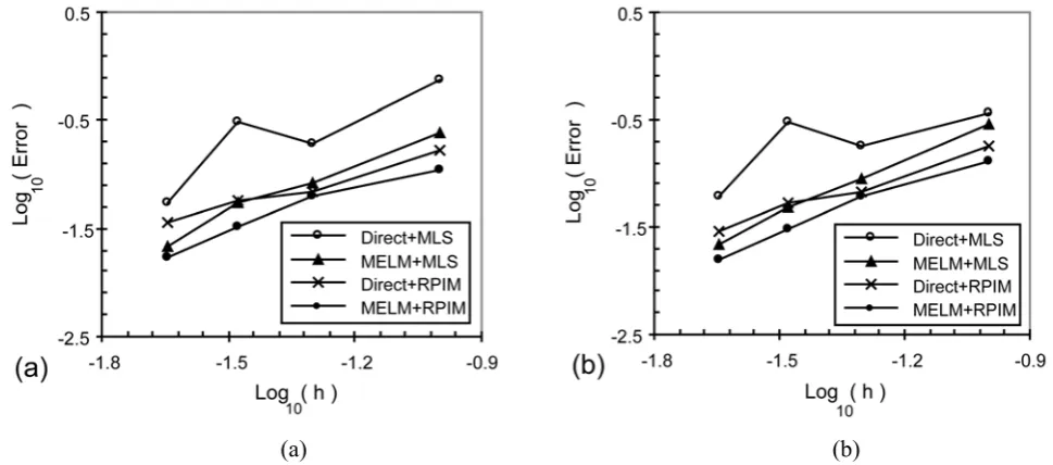
(a) (b) Figure 4. Rate of convergence for closed wave-guide problem with frequency

RPIM interpolation scheme leads to slightly more accurate results.

The distributions of pressure p along the line y = 0.5 m are depicted in Figure 7. As shown in this figure, the results obtained from the modified ELM and the analytical solutions are in a good agreement.

The effects of the width of balanced areas in the modified ELM on the convergence curves are depicted in Figure 8 for a nodal distribution of 441 nodes. In this figure, the error norms for different values of α in Equation 25 are shown. It can be seen that the values in the range between from 0.3 to 0.5 are suitable for α in the considered range.

(a) (b) Figure 5. Rate of convergence for closed wave-guide problem with frequency

f1 = 700 Hz: (a) pressure p and (b) pressure gradient p/x.

(a) (b) Figure 6. Rate of convergence for closed wave-guide problem with frequency

(a)

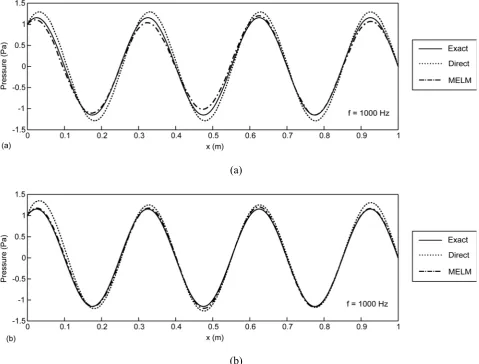
(b)

Figure 7. Distributions of pressure P along the line y = 0.5 for frequency f = 1000 Hz obtained from the direct collocation method

and collocation method with modified ELM using: (a) MLS approximation and (b) RPIM interpolation.

(a) (b)

Figure 8. The error norms of closed wave-guide problem with frequency f1 = 700 Hz for different values of α in the modified ELM:

5.2. Square Cavity

Pa 1 ) 0 , 0 (

p  (39a)

    

    

 

 

 

 

 

 

 

 

 

m 1 y for 2

2 jkp y p

m 0 y for 2

2 jkp y p

m 1 x for 2

2 jkp x p

m 0 x for 2

2 jkp x p

(39b)

The analytical solution of this problem is given as:

)) y x ( 2

2 k sin( j )) y x ( 2

2 k cos( ) y , x (

p     (40)

The problem is solved for three different frequencies f1 = 500 Hz, f2 = 700 Hz and f3 =

1000 Hz. Also, the speed of sound in the media is assumed to be c300 m/s. The calculations are carried out using four regular nodal distributions of 11 × 11, 21 × 21, 31 × 31 and 45 × 45 nodes. The convergence curves for the direct collocation method and modified ELM are plotted in Figures 8-11. Based on these figures, the results obtained from the collocation method with modified ELM are more accurate than those obtained from

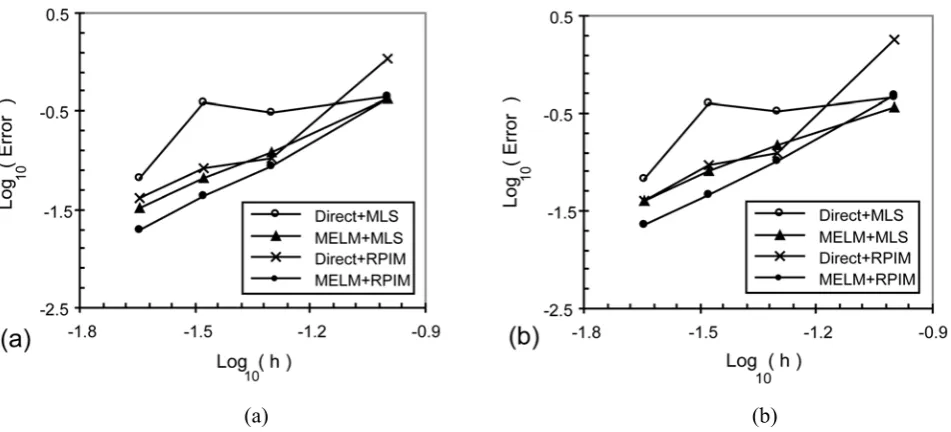
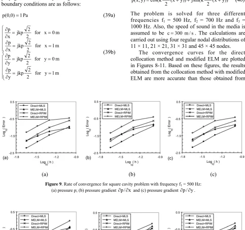
(a) (b) (c) Figure 9. Rate of convergence for square cavity problem with frequency f1 = 500 Hz:

(a) pressure p; (b) pressure gradient p/x and (c) pressure gradient p/y.

(a) (b) (c) Figure 10. Rate of convergence for square cavity problem with frequency f1 = 500 Hz:

the direct collocation method. Also, the modified ELM with RPIM interpolation scheme leads to more accurate results in comparison to the modified

ELM with MLS approximation.

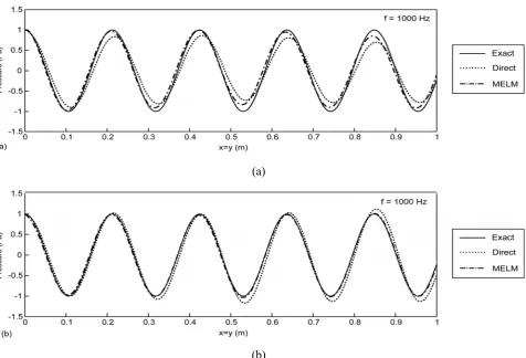
The distributions of pressure p along the diagonal x = y are depicted in Figure 12. As shown

(a) (b) (c) Figure 11. Rate of convergence for square cavity problem with frequency f1 = 1000 Hz:

(a) pressure p; (b) pressure gradient p/x and (c) pressure gradient p/y.

(a)

(b)

Figure 12. Distributions of pressure p along the diagonal x = y for frequency f = 1000 Hz obtained from the direct collocation

in this figure, the results obtained from the modified ELM are more accurate than those obtained from and the direct collocation method.

6. CONCLUSION

In this work, the application of the collocation method with modified ELM is extended for solving two-dimensional acoustic problems. In the modified ELM, equilibrium over the lines on the Neumann (Robin) boundary is satisfied as Neumann (Robin) boundary condition equations. In other words, integration domains are straight lines for nodes located on the Neumann boundary. The performance of the MLS and RPIM interpolations has been examined in this paper. It can be concluded that application of RPIM interpolation leads to more accurate results in comparison to application of the MLS approximation. Numerical studies in section 5 show that the results obtained from the modified ELM are more accurate than those obtained from the direct collocation method.

7. REFERENCES

1. Belytschko, T., Krongauz, Y., Organ, D., Fleming, M. and Krysl, P., “Meshless Methods: An Overview and Recent Developments”, Computer Methods in Applied Mechanics and Engineering,Vol. 139, (1996), 3-47.

2. Liu, G.R., “Meshfree Methods: Moving Beyond the Finite Element Method”, CRC Press, Boca Raton, FL, U.S.A., (2003).

3. Liu, G.R. and Gu, Y.T., “An Introduction to Meshfree Methods and Their Programming”, Springer, Berlin, Germany, (2005).

4. Uras, R.A., Chang, C.T., Chen, Y. and Liu, W.K., “Multiresolution Reproducing Kernel Particle Methods in Acoustics”, Journal of Computational Acoustics,

Vol. 5, (1997), 71-94.

5. Suleau, S. and Bouillard, P.H., “One-Dimensional Dispersion Analysis for the Element-Free Galerkin Method for the Helmholtz Equation”, International Journal for Numerical Methods in Engineering, Vol. 47,

(2000), 1169-1188.

6. Suleau, S., Deraemaeker, A. and Bouillard, P.H., “Dispersion and Pollution of Meshless Solutions for the Helmholtz Equation”, Computer Methods in Applied Mechanics and Engineering, Vol. 190, (2000), 639-657. 7. Lacroix, V., Bouillard, P.H. and Villon, P., “An

Iterative Defect-Correction Type Meshless Method for Acoustics”, International Journal for Numerical Methods in Engineering, Vol. 57, (2003), 2131-2146. 8. Liszka, T.J., Duarte, C.A.M. and Tworzydlo, W.W.,

“Hp-Meshless Cloud Method”, Computer Methods in Applied Mechanics and Engineering, Vol. 139, (1996),

263-288.

9. Liu, G.R. and Gu, Y.T., “A Meshfree Method: Meshfree Weak-Strong (MWS) form Method for 2D Solids”,

Computational Mechanics, Vol. 33, (2003), 2-14.

10. Hu, H.Y., Chen, J.S. and Hu, W., “Weighted Radial Basis Collocation Method for Boundary Value Problems”, International Journal for Numerical Methods in Engineering,Vol. 69, (2007), 2736-2757.

11. La Rocca, A. and Power, H., “A Double Boundary Collocation Hermitian Approach for the Solution of Steady State Convection-Diffusion Problems”,

Computers and Mathematics with Applications, Vol. 55,

(2008), 1950-1960.

12. Sadeghirad, A. and Mohammadi, S., “Equilibrium on Line Method (ELM) for Imposition of Neumann Boundary Conditions in the Finite Point Method (FPM)”, International Journal for Numerical Methods in Engineering, Vol. 69, (2007), 60-86.

13. Sadeghirad, A. and Mahmoudzadeh Kani, I., “Modified Equilibrium on Line Method for Imposition of Neumann Boundary Conditions in Meshless Collocation Methods”, Communications in Numerical Methods in Engineering, Vol. 25, (2009), 147-171.

14. Lancaster, P. and Salkauskas, K., “Surfaces Generated by Moving Least Squares Methods”, Mathematics of Computation, Vol. 37, (1981), 141-158.

15. Wang, J.G. and Liu, G.R., “A Point Interpolation Meshless Method Based on Radial Basis Functions”,