A CHANCE CONSTRAINED INTEGER PROGRAMMING
MODEL FOR OPEN PIT LONG-TERM
PRODUCTION PLANNING
J. Gholamnejad
Department of Mining and Metallurgical Engineering, Yazd University P.O. Box 89195-741, Yazd, Iran
M. Osanloo*
Department of Mining, Metallurgical and Petroleum Engineering, Amirkabir University of Technology P.O. Box 15875-4413, Tehran, Iran
[email protected] - [email protected]
E. Khorram
Department of Mathematical and Computer Science, Amirkabir University of Technology P.O. Box 15875-4413, Tehran, Iran
*Corresponding Author
(Received: August 20, 2007 - Accepted in Revised Form: May 9, 2008)
Abstract The mine production planning defines a sequence of block extraction to obtain the highest NPV under a number of constraints. Mathematical programming has become a widespread approach to optimize production planning, for open pit mines since the 1960s. However, the previous and existing models are found to be limited in their ability to explicitly incorporate the ore grade uncertainty into the planning process. To overcome this shortcoming, this paper presents an Integer Programming (IP) model, for long-term planning of open pit mines. This model is set up to account for grade uncertainty. The grade distribution function, in each block is used as a stochastic input, to optimize the model. The deterministic equivalent of this model is then achieved by using stochastic programming, which is a form of nonlinear in binary variables. Because of the difficulties in solving large scale nonlinear models, the model is then approximated by a linear one.This formulation will yield schedules with high chance of achieving planned production targets, while maximizes the expectation of net present value, it simultaneously minimizes the variance in function.
Keywords Open Pit Mine, Production Planning, Integer Programming, Stochastic Programming
ﻩﺪﻴﻜﭼ
ﯽﻣﺺﺨﺸﻣ ﯼﺭﻮﻃ ﺍﺭ ﻥﺪﻌﻣ ﺯﺍﺎﻫ ﮎﻮﻠﺑ ﺝﺍﺮﺨﺘﺳﺍ ﻑﺩﺍﺮﺗ ﻥﺩﺎﻌﻣ ﺪﻴﻟﻮﺗ ﯼﺰﻳﺭ ﻪﻣﺎﻧﺮﺑ ﺖﺤﺗ ﻪﮐ ﺪﻨﮐ
ﺩﻮﺷﻥﺪﻌﻣﺐﻴﺼﻧﯽﻠﻌﻓﺺﻟﺎﺧﺵﺯﺭﺍﺮﺜﮐﺍﺪﺣ،ﺩﻮﺟﻮﻣﯼﺎﻫﺖﻳﺩﻭﺪﺤﻣ
.
ﻪﻫﺩﺯﺍ ۱۹۶۰ ﻪﻣﺎﻧﺮﺑﺯﺍﻩﺩﺎﻔﺘﺳﺍﯼﺩﻼﻴﻣ
ﻬﺑﺭﺩﯽﺿﺎﻳﺭﯼﺰﻳﺭ ﺖﺳﺍﻩﺪﺷﻝﻭﺍﺪﺘﻣﯽﻠﻴﺧﺪﻴﻟﻮﺗﯼﺰﻳﺭﻪﻣﺎﻧﺮﺑﯼﺯﺎﺳﻪﻨﻴ
. ﻡﺍﺪﮑﭽﻴﻫﺩﻮﺟﻮﻣﻭﯽﻠﺒﻗﯼﺎﻫﻝﺪﻣﺎﻣﺍ
ﺪﻧﺮﻴﮔﺮﻈﻧﺭﺩﺢﻳﺮﺻﺕﺭﻮﺻﻪﺑﺍﺭﯼﺭﺎﻴﻋﺖﻴﻌﻄﻗﻡﺪﻋﺪﻨﺘﺴﻧﺍﻮﺘﻧ
.
ﺢﻴﺤﺻﺩﺪﻋﯼﺰﻳﺭﻪﻣﺎﻧﺮﺑﻝﺪﻣﮏﻳﻪﻟﺎﻘﻣﻦﻳﺍﺭﺩ
ﮔﻅﺎﺤﻟﯼﺯﺎﺳﻝﺪﻣﺭﺩﺭﺎﻴﻋﺖﻴﻌﻄﻗﻡﺪﻋﻪﮐﻩﺪﺷﻪﻳﺍﺭﺍﺯﺎﺑﻭﺭﻥﺩﺎﻌﻣﺕﺪﻣﺪﻨﻠﺑﺪﻴﻟﻮﺗﯼﺍﺮﺑ ﺖﺳﺍﻩﺪﻳﺩﺮ
.
ﻊﻳﺯﻮﺗﻊﺑﺎﺗ
ﺪﺷﻪﺘﻓﺮﮔ ﺮﻈﻧ ﺭﺩﻝﺪﻣﯽﻓﺩﺎﺼﺗﯼﺩﻭﺭﻭﮏﻳ ﻥﺍﻮﻨﻋﻪﺑ ﺎﻫﮎﻮﻠﺑ ﺭﺎﻴﻋﻝﺎﻤﺘﺣﺍ
.
ﯼﺰﻳﺭ ﻪﻣﺎﻧﺮﺑﺯﺍ ﻩﺩﺎﻔﺘﺳﺍﺎﺑ ﺲﭙﺳ
ﺖﺳﺍﯽﻄﺧﺮﻴﻏﻝﺪﻣﮏﻳﻪﮐﺪﺷﻩﺩﺭﻭﺁﺖﺳﺩ ﻪﺑﻥﺁﻝﺩﺎﻌﻣﯽﻌﻄﻗﻝﺪﻣ،ﯽﻓﺩﺎﺼﺗ
.
ﺭﺩﺩﻮﺟﻮﻣﺕﻼﮑﺸﻣﺮﻃﺎﺧﻪﺑ
ﮏﻳﺎﺑﯽﻄﺧﺮﻴﻏﻝﺪﻣ،ﮒﺭﺰﺑﺩﺎﻌﺑﺍﺎﺑﯽﻄﺧﺮﻴﻏﻞﻳﺎﺴﻣﻞﺣ ﺪﺷﻩﺩﺯﺐﻳﺮﻘﺗﯽﻄﺧﻝﺪﻣ
.
ﺍﺭﯼﺍ ﻪﻣﺎﻧﺮﺑﻝﺪﻣﻦﻳﺍ
ﯽﻣﻪﻳﺍﺭﺍﻥﺪﻌﻣﺪﻴﻟﻮﺗﯼﺍﺮﺑ ﺵﺯﺭﺍﻪﮐﯽﻟﺎﺣﻦﻴﻋﺭﺩﻭﻩﺩﻮﺑﺮﺘﺸﻴﺑﻥﺁﺭﺩﯼﺪﻴﻟﻮﺗﻑﺍﺪﻫﺍﻪﺑﯽﺑﺎﻴﺘﺳﺩﺲﻧﺎﺷﻪﮐﺪﻫﺩ
ﯽﻣﻪﻨﻴﺸﻴﺑﻥﺪﻌﻣﯽﻠﻌﻓﺺﻟﺎﺧ ﯽﻣﺶﻫﺎﮐﺰﻴﻧﻥﺁﺲﻧﺎﻳﺭﺍﻭ،ﺩﻮﺷ
ﺪﺑﺎﻳ
.
1. INTRODUCTION
The aim of long-term production planning is, to
grade blending, ore production, mining capacity and etc, during each planning period with the predetermined high degree of probability. Operational Research (OR) techniques have been applied to solve long-term production planning problems since 1960s. There are two mathematical optimization approaches to solve this kind of problems: deterministic and uncertainty-based approaches. In deterministic models all inputs are assumed to have fixed real values (known).
However, the assumption of input certainty is not always realistic. In reality, some data on ore grades, future product demand, price and production costs- can vary within certain limits, (for our discussion, randomly) and we have to make our decision on the production plan before knowing the exact values of those data. None of the deterministic methods are able to deal with the uncertainty in a quantitative manner. This will result in generating infeasible schedules in terms of production requirements.
Uncertainty-based approach in optimizing, open pit mine design and planning has been developed since 1990s. Ravenscroft [1] discussed risk analysis in mine production planning. This method can only show the impact of grade uncertainty on production planning, using the alternative scenarios of the orebody which are provided by conditional simulation. Dowd [2] proposed a framework for risk assessment in open pit mines. He also considered some other random variables like commodity price, mining costs, processing costs, etc. Denby, et al [3] proposed an algorithm which considers ore grade variance in open pit design and planning, using Genetic algorithm. They used multi-objective optimization method: maximizing value and minimizing risk. Dimitrakopoulos, et al [4] discussed an LP approach that considered grade uncertainty, equipment access and mobility constraints. This formulation was based on expected ore block grades and the probabilities of different element grades being above required cutoffs, both were derived from simulated orebody models. Gody, et al [5] presented an algorithm which addresses the generation of optimal condition under uncertainty. At first, they generated production planning on each simulated ore body and then, they combined the mining sequences to produce a single schedule that minimizes the chance of deviating from
production target. This was done using Simulated Annealing Meta-Heuristic method. Ramazan, et al [6] suggested a MIP model that accommodates grade uncertainty. In this method, after obtaining simulated ore body models, planning patterns on each model is generated using traditional MIP formulation (with the objective of NPV maximization). Then the excavation probability of each blocks in a given time period is calculated. The blocks with probability between zero and one, are considered in a new optimization model. It has been shown that these risk-based models are unable to explicitly integrate the ore grade uncertainty and also presenting an optimal solution, under uncertainty without conducting repeated, boring traditional optimization on simulated orebody. To deal with this draw back, a stochastic programming based model is developed by Gholamnejad, et al [7]. In this model, grade uncertainty is incorporated explicitly in the mathematical programming model for long-term production planning by applying chance constrained programming approach. This model generates the schedules that, maximizes net present value of the total revenue and simultaneously, minimizes the risk of the schedules which is originated from ore grade uncertainty, and also maintains a predetermined reliability with respect to satisfying probabilistic constraints. But this model can not be implemented on a large size deposit, owing to the nonlinear form of the objective function and constraints. Therefore accurate linear approximation would be useful to analyze this class of problems.
In this paper, at first the nonlinear integer model for long-term production planning is introduced and then, the nonlinear model is extended by using linear approximation.
2. UNCERTAINTY IN OPEN PIT OPTIMIZATION
because of this, the optimality of the mentioned issues strongly depends on the optimality of the long-term plans. The optimal long-term production plans are sensitive to the uncertainties concerned with the optimization model inputs. The uncertainty related to orebody model and in-situ grade variability is a major contributor, causing expectations not to meet in the early stages of a projects. Valee [8] reported, in the first year of operation after startup, 60 % of surveyed mines had an average rate of less than 70% production of designed capacity. Geological uncertainty is identified as a major contributor to these short falls. Indeed geological risks -which is originated from geological uncertainties, can not be eliminated; consequently, the best solution is to quantify the grade uncertainties, reduce these uncertainties as far as investment permits and finally, manage the residual risk of grade uncertainty.
Kriging is a geostatistical method which estimates the ore block grade so that the mean squared error is minimized; therefore, the variance of value estimated by kriging is smaller than the real but unknown variance. This smoothing of true variability of the grade, leads to overestimation of low grades and underestimation of high grades. Additionally, smoothing is a function of data density and configuration: areas of greater density will show more local variability while areas having sparse data will be more uniform [9]. Hence, production schedules that are based on Kriging can not account for probable deviation in production targets and obtained plans will only provide erroneous conclusions. Multiple Indicator Kriging works on a probabilistic basis to define the distribution of grade of samples within each search window, providing a discrete approximation to the conditional cumulative distribution function for each block [10]. Rather than Kriging, although the probabilistic estimates, produced by Multiple Indicator Kriging method often reduces smoothing effect, but the local grade variability may still be incorrectly characterized.
The best way to quantify grade uncertainty is conditional simulation. Conditional simulation is a generalization of the Monte Carlo type simulation approach, which considers three dimensional spatial correlation [11,12]. It produces independent and equally probable images of in-situ orebody grades
which have the following characteristics [13]: • At sampled location, the simulated values of
each variable are the same as measured values of those variables.
• All the simulated values of a given variable have the same spatial relationships as observed in the data value.
• All the simulated values of any pairs of variables have the same spatial interrelationships as observed in the data values.
• The simulated values histogram, of all variables are the same as those observed for the data images.
Each simulation run produces an image or a realization of the deposits that correctly reflects the statistical and spatial variability of the real data. Performing several independent simulations are required to assess the impact of local variability. Reducing the uncertainty of the ore blocks grade can be achieved by spending more money to increase drill holes density. These infill drilling should be conducted preferably in the high grade zones associated with a high level of uncertainty. These zones can be identified by using results of conditional simulation.
Finally mine planning should be managed in such a way, so that the residual risk of grade uncertainty is minimized in design procedure. The key note in this regard is, the extraction of high grade and certain low zones in earlier production periods, and leaving more uncertain zones for the later periods such as, all mining constraints are satisfied with a high level of confidence. In the following sections we deal with this important using Stochastic Programming.
3. STOCHASTIC VERSION OF LONG-TERM PRODUCTION PLANNING MODEL
Stochastic programming based production planning method can be summarized as follows:
• To develop an economic block model.
[14,15] and maximum flow network methods [16,17].
• To develop a stochastic integer programming model for optimal selection of the blocks in each period on the basis of specified criteria. • Obtaining the deterministic equivalent on
mentioned stochastic model.
• Solving the deterministic form of the stochastic model for long term production planning problem using efficient zero-one integer programming methods.
4. FORMULATION OF THE LONG-TERM PRODUCTION PLANNING PROBLEM
The following variables are defined for the mathematical formulation of the long term production planning model:
t: Planning period index, t = 1,2,…,T. T: Total number of planning periods in
the planning horizon.
n: Block identification number; n = 1,2,…,N.
N: Total number of blocks to be scheduled.
d: Discount rate in each period.
xnt: A binary decision variable which is equal to 1 if the block i is to be mined in period t and 0 otherwise. Pt: Unit selling price of the metal in
period t.
SPt: Unit selling cost of the metal in period t.
Pct: Unit processing cost of the ore in period t.
Mcot: Unit mining cost of the mineralized material in period t.
Mcwt: Unit mining cost of the waste/overburden material in period t. n
g~ : Block grade which is a random variable (n = 1,2,…,N).
E(g~n): Expected value of g~n. Var(g~n): Variance estimation of g~n. Cov(g~n,g~m): Covariance between g~n and g~n. Cnt: Net present value to be generated by
mining block n in period t.
⎭ ⎬ ⎫ ⎩
⎨
⎧ −
⎥⎦ ⎤ ⎢⎣
⎡ − − −
+ =
) n .Tw t cw (M n .To t co M t c P .R n g~ ). t SP t (P
t d) (1
1 t n C
(1)
R: Total metal recovery.
Ton: The total amount of ore in block n. Twn: The total amount of waste in block n. Gmaxt: The upper bound average grade of
material sent to the mill in period t. Gmint: The lower bound average grade of
material sent to the mill in period t. PCmaxt: The upper bound total tones of ore
processed in period t.
PCmint: The lower bound total tones of ore processed in period t.
MCmaxt: The upper bound total amount of material (waste and ore) to be mined in period t.
MCmint: The lower bound total amount of material (waste and ore) to be mined in period t.
b: The index of a block considered for extraction in period t.
e: The total number of blocks
overlaying block b.
l: The counter for the m overlaying blocks.
αt: The least probability of fulfilling the demand in period t (confidence level). As a matter of fact 1-αt represent the acceptable risk level for not fulfilling the demands in period t. Pr: The probability operator.
4.1. Formulation of the Multi-Period
Long-Term Production Planning Model
In light ofdefinition described above, the multi-period production planning model will be formulated as follows:
4.1.1. Objective function
∑ = ∑= = T
1 t
N
1 n
t n .x t n C Z
Maximize (2)
constraints:
4.1.2. Grade blending constraints The average
grade of the mineralized material sent to the mill has to be more than a lower bound (Gmint) and less than an upper bound (Gmaxt) in each period:
t max G N
1 n
t n .x n To N
1 n
t n .x n .To n
g~ ∑ ≤
= ∑
=
t = 1,2,…,T (3)
t min G N
1 n
t n .x n To N
1 n
t n .x n .To n
g~ ∑ ≥
= ∑
=
For t = 1,2,…,T (4)
4.1.3. Processing capacity constraints The total
tones of ore processed in each period should be more than a lower bound (PCmint) and less than an upper bound (PCmaxt):
t max PC N
1 n
t n .x n
To ≤
∑ =
For t = 1,2,…,T (5)
t min PC N
1 n
t n .x n
To ≥
∑ =
For t = 1,2,…,T (6)
4.1.4. Mining capacity constraints The total
tones of waste and ore to be mined should be more than a lower bound (MCmint) and less than an upper bound (MCmaxt):
t max MC N
1 n
t n )x n Tw n
(To ≤
∑
= +
For t = 1,2,…,T (7)
t min MC N
1 n
t n )x n Tw n
(To ≥
∑
= +
For t = 1,2,…,T (8)
4.1.5. Reserve constraints Reserve constraints
insure that any block in the model mined only
once:
∑
= =
T
1
t 1
t n x
For n = 1,2,…,N (9)
4.1.6. Slope constraints These constraints insure
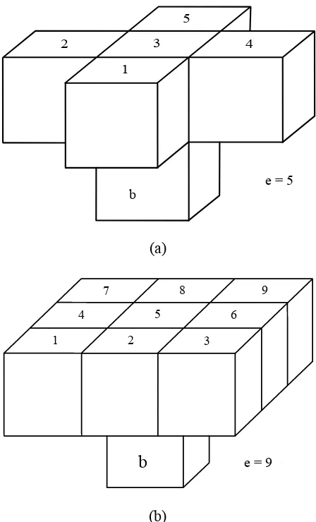
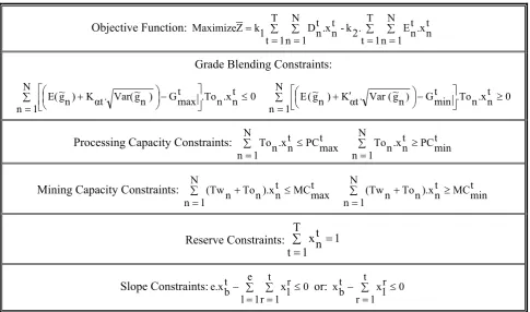
that all blocks which directly restrict the mining of a given block b must be completely mined out before the mining of block b starts. To represent the restricting blocks a cone template can be made either contains 5 (Figure 1a) or 9 blocks (Figure 1b) above block b. In this study a cone template with 9 blocks will be used. There are two methods for implementing these constraints [18]:
Using one constraint for each block per period:
∑
= ∑= ≤ − e
1
l 0
t
1 r
r l x t
b e.x
For t = 1,2,…,T, b = 1,2,…,N (10) Using e constraints for each block per period:
0 t
1 r
r l x t
b
x ∑ ≤
= −
For t = 1,2,…,T,
b = 1,2,…,N, l = 1,2,...,e (11) Ramazan and Dimitrakopoulos showed that in large size models it may be better to use Equation 11 [19]. Although using Equation 14 will increase the size of the model, but in some cases it may significantly decrease the computing time by decreasing the search space.
4.2. Stochastic Formulation of the
Multi-Period Long-term Production Planning
Model
As mentioned before, ore block’s gradei
1
2 3 4
5
b
e=5
(a)
i
1 2 3
4 5 6
7 8 9
b
e=9
(b)
Figure 1. Two types of cone templates to model the slope constraints.
There are several approaches to handle uncertainty of this problem. The two most common approaches are; Two stage stochastic programming method and Chance-constrained stochastic programming method. In the first apprroach, decision maker takes some action in the first place, after which a random event occurs affecting the outcome of the first stage decisions. A recourse decision can then be made in the second stage that would compensates for any adverse outcome that might have been experienced as a result of the first-stage decision. Constraints violation caused by unexpected random effects, can be balanced afterwards, by some compensating decisions in second stage. As long as the costs of compensating
decisions are known, these may be considered as a penalization for constraint violation. In this method the stochastic constraints have to be surely held, i.e., they are to be satisfied with probability of one [21]. In many applications, however, compensations simply do not exist or can not be modeled as costs in any reasonable way. In such circumstances, one would rather insist on decisions guaranteeing feasibility “as much as” possible. This loose term refers once more to the fact that constraints violations, can almost never be avoided because of the extreme events, i.e., a low percentage realization of the random parameters, leads to constraints violation under this fixed decisions. This approach is called chance constrained programming.
Chance-constrainted programming was formulated originally by Charnes, et al [22,23] and then developed and applied by Charnes, et al [24]. In this section the chance constrained programming approach is exploited to handle block grade uncertainty for the proposed binary integer model.
As stated before, among the model constraints only constraints 3 and 4 contain random parameters. The generic way to express such constraints is:
t
α
t max G N
1 n
t n .x n To N
1 n
t n .x n .To n g~
Pr ≥
⎥ ⎥ ⎦ ⎤ ⎢
⎢ ⎣ ⎡
≤ ∑
= ∑
=
For t = 1,2,…,T (12)
t
α
t min G N
1 n
t n .x n To N
1 n
t n .x n .To n g~
Pr ≥
⎥ ⎥ ⎦ ⎤ ⎢
⎢ ⎣ ⎡
≥ ∑
= ∑
=
For t = 1,2,…,T (13)
The value of αt ∈ [0,1]is called the probability level, and it is chosen by the decision maker in order to model the safety requirements. It should be noted that higher values of αt results in fewer feasible solutions xit in constraints 17 and 18, hence yields optimal solution at lower NPV. Henrion stated that usually αt can be increased over quite a wide range without affecting too much the optimal value of some problem, until it closely approaches 1 and then a strong decrease of NPV becomes evident [25].
e = 5 b
With regard to the stochastic nature of the objective function and also constraints 12 and 13, above problem is not well defined; consequently, a revision of modeling process is necessary, leading to so-called deterministic equivalents for stochastic programming model, i.e. one which does not contain any probabilistic element any more.
4.3. Deterministic Equivalent of Chance
Constrained Binary Integer Programming
Model
In this section the chance constrainedbinary integer programming model of long-term production planning problem is reduced to its deterministic equivalent.
4.3.1.
Objective function As is clear fromequation 2 due to stochastic nature of Ctn, Z is also a random variable with the expected value and variance of: ⎭ ⎬ ⎫ ⎥⎦ ⎤ − − ∑ = ∑= ⎩⎨ ⎧ ⎢⎣ ⎡ − − + = t n .x ) t cw .M n (Tw n ].To t co M t c P T 1 t N 1 n R . ) n g~ E( . ) t SP t [(P t d) (1 1 (Z) E (14) m n ) m g~ , n g~ .Cov( t m .x t n .x m .R.To t SP t P T 1 t N 1 n N 1 m n .R.To t SP t P ) n g~ .Var( T 1 t N 1 n 2 t n .x n .R.To t SP t P 2t d) (1 1 Var(Z) ≠ ⎭ ⎬ ⎫ ⎥⎦ ⎤ ⎢⎣ ⎡ ⎟ ⎠ ⎞ ⎜ ⎝ ⎛ − ∑ = ∑= ∑= ⎥⎦× ⎤ ⎢⎣ ⎡ ⎟ ⎠ ⎞ ⎜ ⎝ ⎛ − + ⎪⎩ ⎪ ⎨ ⎧ ∑ = ∑= ⎥⎦ ⎤ ⎢⎣ ⎡ ⎟ ⎠ ⎞ ⎜ ⎝ ⎛ − + = (15) Several classes of objective function can be
identified which result in different solutions. These include [24]:
• Expected value optimization objective • A minimum variance objective • A maximum probability model
We setup our objective to maximization of expected value of net present value and minimization of standard deviation simultaneously; as a result, the objective function of open pit
long-term production planning can be written as:
) Z ( Var . k ) Z ( E . k Z
Maximize = 1 − 2 (16)
Where k1 and k2 are nonnegative coefficients and reflect the relative importance of maximization of expected value and minimization of standard deviation of net present value. If k1 = k2 then these two objectives are of the same importance for the decision maker. Thus the objective function can be re-written as follows:
m n 2 1 )} m g~ , n g~ .Cov( t m .x t n .x m R.To . ) t SP t (P T 1 t N 1 n N 1
m ).R.Ton
t SP t (P ) n g~ .Var( T 1 t N 1 n 2 t n .x n ).R.To t SP t (P { 2t d) (1 1 2 k t n )).x t cw .M n (Tw n ].To t co M t c P ).R n g~ .E( T 1 t N 1 n ) t SP t (P ([ t d) (1 1 . 1 k Z Maximize ≠ ⎥⎦ ⎤ ⎥⎦ ⎤ ⎢⎣ ⎡ − ∑ = ∑= ∑= ⎥⎦× ⎤ ⎢⎣ ⎡ − + ⎢ ⎢ ⎣ ⎡ ∑ = ∑= ⎥⎦ ⎤ ⎢⎣ ⎡ − + − ⎭ ⎬ ⎫ ⎥⎦ ⎤ − − − ∑ = ⎪⎩ ⎪ ⎨ ⎧ ∑ = ⎢⎣ ⎡ − + = (17) In zero-one integer programming we have
t i x 2 t i x ⎟ =
⎠ ⎞ ⎜ ⎝
⎛ ; because of this, the final shape of objective function has a form of:
m n 2 1 )} m g~ , n g~ .Cov( t m .x t n .x m .R.To t SP t P T 1 t N 1 n N 1
m .R.Ton
t SP t P ) n g~ .Var( t n .x T 1 t N 1 n 2 n .R.To t SP t P { 2t d) (1 1 2 k t n )).x t cw .M n (Tw n ].To t co M t c P ).R n g~ .E( T 1 t N 1 n ) t SP t (P [ ( t d) (1 1 . 1 k Z Maximize ≠ ⎥⎦ ⎤ ⎥⎦ ⎤ ⎢⎣ ⎡ ⎟ ⎠ ⎞ ⎜ ⎝ ⎛ − ∑ = ∑= ∑= ⎥⎦× ⎤ ⎢⎣ ⎡ ⎟ ⎠ ⎞ ⎜ ⎝ ⎛ − + ⎢ ⎢ ⎣ ⎡ ∑ = ∑= ⎥⎦ ⎤ ⎢⎣ ⎡ ⎟ ⎠ ⎞ ⎜ ⎝ ⎛ − + − ⎭ ⎬ ⎫ ⎥⎦ ⎤ − − − ∑ = ⎪⎩ ⎪ ⎨ ⎧ ∑ = ⎢⎣ ⎡ − + = (18)
will obtain the deterministic equivalents of stochastic constraints. In Equation 12 and 13 let us define:
∑ = ∑ = = N 1 n t n .x n To N 1 n t n .x n .To n g~ t
d (19)
Thus, Equation 12 can be re-written as:
t α t max G t d Pr ≥ ⎥⎦ ⎤ ⎢⎣ ⎡ ≤
For t = 1,2,…,T (20)
As mentioned before,
d
tis the average grade of blocks to be scheduled in period t which is a random variable. According to the Central Limit Theorem, the distribution of dt can be approximated by a normal distribution function with the following mean and variance:∑ = ∑ = = N 1 n t n .x n To N 1 n t n .x n ).To n g~ E( ) t
E(d (21)
2 N 1 n t n .x n To N 1 n N 1 m ) m g~ , n g~ Cov( . ) t m .x m To ( ) t n .x n To ( N 1 n t n ).x n g~ ( .Var 2 n To ) t Var(d ⎥ ⎥ ⎦ ⎤ ⎢ ⎢ ⎣ ⎡ ∑ = ∑ = ∑= + ∑ = = (22)
if we minus E(dt) from both side of Equation 20, and then divide by var(dt), it can be re-written as:
t α ) t Var(d ) t E(d t max G ) t Var(d ) t E(d t d Pr ≥ ⎥ ⎥ ⎥ ⎦ ⎤ ⎢ ⎢ ⎢ ⎣ ⎡ − ≤ − (23) By defining ) t Var(d ) t E(d t d t
D = − , then Dt has a standard normal distribution function which has a zero mean and unit standard deviation. A value of Kat can then be determined from the area under normal curve such that:
t α dx ) 2 2 x .exp( αt K 2π 1 ) αt K t
Pr(D ∫ − =
∞ − =
≤ (24)
Thus, combining Equations 23 and 24 yields:
t max G ) t Var(d αt K ) t (d E αt K ) t Var(d ) t E(d t max G ≤ + ⇒ ≥ − (25)
With the combination of Equations 21, 22 and 25 the deterministic equivalent form of constraints 12 can be stated as follows:
0 N 1 n N 1 m ) m g~ , n g~ Cov( . ) t m x . m To ( ) t n .x n To ( N 1
n .Var(g~n)
t n x . 2 ) n (To . αt K N 1 n t n x . n To . ) t max G ) n g~ ( E ( ≤ ∑ = ∑= ∑ = + ∑ = − + (26) Similarly, the deterministic equivalent of Equation
13 is of the form:
0 N 1 n N 1 m ) m g~ , n g~ .Cov( ) t m .x m To ( ) t n .x n To ( N 1 n ) n g~ .Var( t n .x 2 ) n (To N 1
n Kαt.
t n .x n .To ) t min G ) n g~ E( ( ≥ ∑ = ∑= ∑ = + ∑ = − + ′ (27) Where: t α -1 dx ) 2 2 x ( exp . αt K 2π 1 ) αt K t D (
Pr ∫ − =
′
∞ − = ′
≤ (28)
it is clear from the above relations, the deterministic equivalents of probabilistic constraints are nonlinear. However, other constraints are themselves deterministic and remain unchanged.
4.4. Linearization of the Nonlinear Model
for Long Term Production Planning
Aprogramming is the need for a nonlinear algorithm. In this section linear approximation method is used for solving the nonlinearity of the problem; therefore, the objective will be, to linearize the functions and constraints so that linear programming algorithms can be used.
Suppose that xi and xj are two dependent random variables. The definition of the correlation between variables xi and xj is:
) j Var(x ) i Var(x ) j x , i Cov(x ij ρ ×
= (29)
Since −1≤ρij≤1,
1 ) j Var(x ) i Var(x ) j x , i Cov(x 1 ≤ × ≤
− (30)
Therefore: ) j Var(x ) i Var(x ) j x , i Cov(x ) j Var(x ) i Var(x × ≤ ≤ × − (31)
This means that the maximum amount of the covariance of two variables would be the product of standard deviation of each. Hence replacing cov(xi,xj) with Var(xi)× Var(xj) in Equation 18 and considering x12+x22+...+x2n ≤
n x ... 2 x 1
x + + + (where x1,x2,...,xn are positive variables) the linear equivalent of the objective function can be written as:
m n T 1 t N 1
n ). Var(g~n)
t n .x n To ( R. . ) t SP t P ( 2t d) (1 1 . 2 k t n )).x t cw .M n (Tw n ].To t co M t c P ).R n g~ ( E . T 1 t N 1 n ) t SP t P ( [ ( t d) (1 1 . 1 k Z Maximize ≠ ⎪⎭ ⎪ ⎬ ⎫ ⎪⎩ ⎪ ⎨ ⎧ ∑ = ⎟ ⎟ ⎠ ⎞ ⎜ ⎜ ⎝ ⎛ ∑ = ⎥⎦ ⎤ ⎢⎣ ⎡ − + − ⎭ ⎬ ⎫ ⎥⎦ ⎤ − − − ∑ = ⎪⎩ ⎪ ⎨ ⎧ ∑ = ⎢⎣ ⎡ − + = (32) Let define: n To . .R ) n g~ ( Var . ) t SP t P ( . t d) (1 1 t n E ) t cw M . n Tw ( n To . t co M t c P R . ) n g~ ( E . ) t SP t P ( t d) (1 1 t n D ⎥⎦ ⎤ ⎢⎣ ⎡ − + = ⎟ ⎠ ⎞ − ⎜ ⎝ ⎛ ⎥⎦ ⎤ ⎢⎣ ⎡ − − − + = (33) Thus the objective function can be simplified as:
∑ = ∑= ∑ = ∑= − = T 1 t N 1 n t n .x t n E . 2 k T 1 t N 1 n t n .x t n D 1 k Z Maximize (34)
As can be seen from the Equation 34 the final shape of objective function has a linear form. Similarly, the upper bound of Var(dt) can be achieved by replacing cov(xi,xj) with Var(xi)× Var(xj) in Equation 22:
2 N 1 n t n .x n To 2 N 1 n t n .x ) n g~ Var( . n To 2 N 1 n t n .x n To N 1 n N 1
m ).Var(g~n).Var(g~m)
t m .x m (To ) t n .x n To ( N 1 n t n ).x n g~ .Var( 2 n To 2 N 1 n t n .x n To N 1 n N 1
m ).Cov(g~n,g~m)
t m .x m (To ) t n .x n To ( N 1 n t n ).x 9n g~ .Var( 2 n To ) t Var(d ⎥ ⎥ ⎦ ⎤ ⎢ ⎢ ⎣ ⎡ ∑ = ⎥ ⎥ ⎦ ⎤ ⎢ ⎢ ⎣ ⎡ ∑ = = ⎥ ⎥ ⎦ ⎤ ⎢ ⎢ ⎣ ⎡ ∑ = ∑ = ∑= + ∑ = ≤ ⎥ ⎥ ⎦ ⎤ ⎢ ⎢ ⎣ ⎡ ∑ = ∑ = ∑= + ∑ = = (35) by combining relations 21, 25 and 35 the upper
bound grade blending constraints can be written as:
TABLE 1. The Final Form of Long-Term Production Planning Problem in a Stochastic Environment.
Objective Function: ∑
= ∑= ∑
= ∑=
= T
1 t
N
1 n
t n .x t n E .
2 k T
1 t
N
1 n
-t n .x t n D 1
k Z Maximize
Grade Blending Constraints:
0 N
1 n
t n .x n .To t max G ) n g~ Var( .
αt
K ) n g~
E( ≤
∑
= ⎥⎦
⎤ ⎢⎣
⎡ −
⎟ ⎠ ⎞ ⎜
⎝
⎛ + N 0
1 n
t n .x n .To t min G ) n g~ ( Var .
αt
K ) n g~ (
E ≥
∑
= ⎥⎦
⎤ ⎢⎣
⎡ ⎟−
⎠ ⎞ ⎜
⎝
⎛ + ′
Processing Capacity Constraints: N PCtmax 1
n
t n .x n
To ≤
∑
=
t min PC N
1 n
t n .x n
To ≥
∑ =
Mining Capacity Constraints: N MCtmax 1
n
t n ).x n To n
(Tw ≤
∑
= +
t min MC N
1 n
t n ).x n To n
(Tw ≥
∑
= +
Reserve Constraints: ∑
= =
T 1 t
1 t n x
Slope Constraints: ∑
= ∑= ≤
− e
1
l 0
t
1 r
r l x t
b
e.x or: t 0
1 r
r l x t
b
x ∑ ≤
= − or
0 N
1 n
t n .x n .To t
max G ) n g~ Var( .
αt
K ) n g~
E( ≤
∑
= ⎥⎦
⎤ ⎢⎣
⎡ ⎟−
⎠ ⎞ ⎜
⎝
⎛ +
(37) Similarly, the lower bound grade blending
constraints is converted to the following inequality:
0 N
1 n
t n .x n .To t min G ) n g~ ( Var . αt K ) n g~
E( ≥
∑
= ⎥⎦
⎤ ⎢⎣
⎡ −
⎟ ⎠ ⎞ ⎜
⎝
⎛ + ′
(38) Hence using this approximation, objective function
and grade blending constraints are linearized. It should be noted that this linear approximation would involve less error if positive covariance existed, because in this case cov(xi,xj) is nearer to
) j Var(x )
i
Var(x × . Clearly, the error would be greater in the case of negative covariance. Also linear approximation in constraints 37 and 38 are
tighter than their nonlinear form; consequently, linear approximation is more conservative than that of nonlinear original.
The final form of long-term production planning problem in a stochastic environment is summarized in Table 1.
Therefore, the final shape of long term production planning with regard to grade uncertainty has a linear form with zero-one variables. Now this model can be solved by Branch and Bound, Cutting Plane and Branch and Cut techniques.
5. CONCLUSION
production and also schedules' to meet the required targets, with a high level of confidence and low risk. At first, a probabilistic form of the long term production planning model was developed, which containd a stochastic objective function and a series of deterministic and stochastic constraints. The stochastic objective function and also constraints could not be handled directly in the optimization process; consequently, using chance constraints, a deterministic form of the model was obtained. This process led to converting stochastic linear equations to deterministic nonlinear equivalents. In this model objective function and grade blending constraints are nonlinear. Because of the difficulties in solving large scale nonlinear models, a linearization process was applied and nonlinear functions are approximated by linear ones. The resultant linear model can be solved by using popular linear zero-one programming algorithms; therefore, this model can be applied in large size open pit mines. The results obtained from this model seems to be more economical in the long run, than those obtained from the previous models, because the objective function will force the model to derive the mining sequence through zones, where the risk of not achieving the production targets, is minimized; therefore, the resultant schedule is feasible in terms of meeting the production targets with a high level of confidence.
6. REFFERNCES
1. Rovenscroft, P. J., “Risk Analysis for Mine Planning by Conditional Simulation”, Trans. Instn Min. Metall., (Sec. A: Min. Industry), The Institution of Mining and Metallurgy, Vol. 101, (May-August 1992), A82-A88.
2. Dowd, P. A., “Risk Assessment in Reserve Estimation and Open Pit Planning”, Trans. Instn Min. Metall., (Sec. A: Min. Industry), The Institution of Mining and Metallurgy, Vol. 103, (September-November 1994), A148-A154.
3. Denby, B. and Schofield, D., “Inclusion of Risk Assessment in Open Pit Design and Planning”, Trans. Instn. Min. Metall., (Sec. A: Min. Industry), The Institution of Mining and Metallurgy, Vol. 104, (January-April 1995), A67-A71.
4. Dimitrakopoulos, R. and Ramazan, S., “Uncertainty based production scheduling in open pit mining”, SME Annual Meeting and Exhibit, Cincinnati Ohio, U.S.A., Vol. 316, (February 24-26, 2003), 106-112.
5. Godoy, M. and Dimitrakopoulos, R., “Managing Risk and Waste Mining in Long-Term Production Planning of Open Pit Mine”, SME Annual Meeting and Exhibit, Cincinnati Ohio, U.S.A., Vol. 316, (February 24-26, 2003), 43-50.
6. Ramazan, S. and Dimitrakopoulos, R., “Traditional and New MIP Models for Production Planning with in-Situ Grade Variabulity”, International Journal of Surface Mining, Reclamation and Environment, Vol. 18, No. 2, (2003), 85-98.
7. Gholamnejad, J., Osanloo, M. and Karimi, B., “A Chance-Constrained Programming Approach for Open Pit Long-Term Production Scheduling in Stochastic Environments”, The Journal of the South African Institute of Mining and Metallurgy, Vol. 106, (2006), 105-114.
8. Vallee, M., “Mineral Resource + Engineering, Economic and Legal Feasibility = Ore Reserve”, CIM Bulletin, Vol. 90, (2000), 53-61.
9. Smith, M. L., “Integrating Conditional Simulation and Stochastic Programming: an Application in Production Planning”, Proceeding of Application of Computers
and Operations Research in the Mineral Industry,
(2001), 230-207.
10. David, M. A., “Hand Book of Applied Advanced Geostatistical Ore Reserve Estimation”, Elsevier Scientific Publisher, Nehterland, (1988).
11. Journel, A. G. and Huijbregts, C., “Mining Geostatistics”, Academic Press, New York, U.S.A., (1978), 600.
12. Dowd, P. A., “A Review of Recent Developments in Geostatstics”, Computers and Geostatistics, Vol. 17, No. 10, (1992), 1481-1500.
13. Dowd, P. A., “Risk In Minerals Projects: Analysis, Perception and Management”, Trans. Instn Min. Metall., (Sec. A: Min. Industry), The Institution of Mining and Metallurgy, Vol. 106, (January-April 1997), A9-A18.
14. Lerchs, H. and Grossman, F., “Optimum Design of Open-Pit Mines”, Transaction CIM, Vol. 58, No. 633, (1965), 47-54.
15. Zhao, H. and Kim, Y. C., “A New Optimum Pit Limit Design Algorithm”, 23rd International Symposium on The Application of Computers and Operations Research in the Mineral Industries, AIME, Littleton, Co, (1992), 423-434.
16. Johnson, T. B. and Barnes, J., “Application of Maximal flow Algorithm to Ultimate Pit Design”, Engineering Design: Better Results through Operations Research Methods. North Holland, (1988), 518-531.
17. Yegulalp, T. M. and Arias, J. A., “A Fast Algorithm to Solve Ultimate Pit Limit Problem”, 23rd International Symposium on the Application of Computers and Operations Research in the Mineral Industries, AIME, Littleton, Co, (1992), 391-398.
19. Ramazan, S. and Dimitrakopoulos, R., “Recent Applications of Operations Research in Open Pit Mining”, SME Annual Meeting and Exhibit, Cincinnati Ohio, U.S.A., Vol. 316, (February 24-26, 2003), 73-78. 20. Gangwar, A., “Using Geostatistical Ore Block Variance
in Production Planning by Integer Programming”, 17th
APCOM Symposium, (1982), 443-460.
21. Kall, P. and Wallace, S. W., “Stochastic Programming”, First Edition, John Wiley and Sons, Chichester, England, (1994), 50-95.
22. Charnes, A., Cooper, W. W. and Symonds, G. H., “Cost Horizons and Uncertainty Equivalents: an Approach to Stochastic Programming of Heating Oil”, Management Science, Vol. 4, No. 3, (April 1958), 235-263.
23. Charnes, A. Cooper, W. W., “Chance-Constrained Programming”, Management Science, Vol. 6, (1959), 73-79.
24. Charnes, A. and Coper, W. W., “Deterministic Equivalents for Optimizing and Satisficing under Chance-Constraints”, Operation Research, Vol. 11, (1963), 18-39.
25. Henrion, R., “Introduction to Chance-Constrained Programming”, Http://Stoprog.Org/Spintro/INTRO2CCP. HTML, (September 15, 2005).