International Journal of Engineering
J o u r n a l H o m e p a g e : w w w . i j e . i r
Simulation of Store Separation using Low-cost CFD with Dynamic Meshing
M. Jafari a, A. Toloei* a, S. Ghasemlu b, H. Parhizkar b
a Department of New Technologies Engineering, Shahid Beheshti University, Tehran, Iran b Department of Aerospace Engineering, Amirkabir University, Tehran, Iran
P A P E R I N F O
Paper history: Received 26 January 2013
Received in revised form 06 October 2013 Accepted 07 November 2013
Keywords: Store Separation Automatic Coupling Dynamic Mesh Quasi Static
Time Dependent Solution Low-cost CFD
A B S T R A C T
The simulation of the store separation using the automatic coupling of dynamic equations with flow aerodynamics is addressed. The precision and cost (calculation time) were considered as comparators. The method used in the present research decreased the calculation cost while limiting the solution error within a specific and tolerable interval. The methods applied to model the aerodynamic forces are time-dependent dynamic meshes and quasi-static methods. In the time-time-dependent method, a dynamic unstructured tetrahedral mesh approach using combination of spring-based smoothing and local remeshing is employed in respect of bodies motion with an implicit, second-order upwind accurate 3-D Euler solver. In this method, a 6dof dynamic code is coupled with the flow solver to update the store trajectory information. In the quasi-static method, a 3-D implicit, steady state Euler solver is automatically integrated with a grid generation software and a 6dof dynamic code. Although the time-dependent method is more precise and reliable, it is not proper and appropriate for the initial design of the separation system due to its high cost. The quasi-static solution is very fast, but unable to simulate realistically because of not satisfying the problem conditions due to solution divergence as the store speed increases. The method used in the present research decreased the calculation cost while limiting the solution error within a specific and tolerable interval. In this way, the time step can be enlarged, the solution can be carried out with a few calculation points, and the solution can have considerably more speed with a limited error magnitude. Simulation of the store separation using the automatic coupling of dynamic equations with flow aerodynamics with the new Low-Cost method is the innovative aspect of this paper. To validate the solution method, the transonic store separation was simulated that agreed well with the wind tunnel test outcomes.
doi:10.5829/idosi.ije.2014.27.05b.14
1. INTRODUCTION1
Gaining knowledge about how to release a store from an airplane, with sufficient immunity and precision in striking the target has significant importance. In addition to the wind tunnel and flight test, the computerized simulation has been recently used to reduce simulating costs [1]. Several analyses have been carried out to properly simulate separation from the airplane body. A separation analysis was performed by Parikh et al. [2] and Meakin [3] on a wing-pylon-store. The Euler’s and Navier-Stokes solutions for the thin layer were in good accordance with the wind tunnel outcomes. Additional analyses were also performed for the same problem using Overflow [4] and Fastran [5]
*Corresponding Author Email: [email protected] (Alireza Toloei)
softwares. Recent analyses have also been executed based on the Cartesian method [6]. Approximate quasi-static methods have also been applied in addition to the exact time dependent procedure [6-8]. Due to fine meshing and small time steps to reach the needing precision, the solution cost, i.e. time, is rather high in numerical methods [9]. The viscosity of the flow has minor effect on the cold separation analysis, specifically with the absence of gas dynamic effects. Therefore, the calculation time can be considerably reduced by neglecting viscosity [9].
parameters including the separating force, the safe separation altitude and velocity, etc. are unknown in newly designed separating systems, so scanning through the designing tables increases the solution time. In the present method, the so-called parameters can be estimated and exactly obtained after the solution procedure.
2. PROBLEM DESCRIPTION
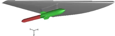
As stated above, the present research aims at approxi-mating the trajectory of a separated store from the airplane in the wing- pylon-store model, as shown in Figure 1. The indicated model is similar to the experimental test specimen in literature. [10].
The coordinate origin before separation is located in the mass center. The wing in the present model is a clip-ped delta, and it has an NACA64A010 airfoil section. The store has four NACA008 bulks (with constant widths) in its tail, with a total length of 9.9 ft. In order to assimilate the model with the experimental specimen, a 0.12 ft is provided between the store body and the pylon before separation. Finally, like the experimental specimen, a 1.17 ft sting is added to the end of the store [1].
3. SOLUTION METHOD
The solution method consisted of three stages: the flow solution, the trajectory calculation, and the meshing algorithm. The flow solver is used to solve the governing fluid dynamic equations in each and every time step. The aerodynamic forces and moments on the adjoining store are calculated by integrating the surface pressure. By knowing the aerodynamic and other exter-nal forces, the displacement of the store will be obtained with six degrees of freedom. Ultimately, the mesh will be modified according to the store displacement using the meshing algorithm.
4. FLOW SOLVER
The solution of the flow field is carried out using Euler equations based on the finite volume method [11, 12].
Figure 1. The outline of the wing- pylon- adjunct model
As stated earlier, the flow viscosity has been neglected for the sake of having less calculation time. The outline of the solution algorithm is shown in Figure 2. This figure indicates that the calculation program yields the aerodynamic forces and moments in each and every time step by having the store locality. Using the obtained forces and moments, together with other external forces, the linear and angular velocities are updated and the mesh will be modified accordingly.
5. CALCULATION OF THE TRAJECTORY
The aerodynamic forces and moments are calculated by integrating into the surface pressure while the flow viscosity, and thus the corresponding stresses, are neglected in Euler’s solution. These data will be obtained from the flow solver in the inertial system and are used for simulation with 6 degrees of freedom. The governing equation system for the translation of the mass center is [1]:
G
vr& =m
å
fGr (1)The moments can be transferred into the body system from the inertial system using the translation matrix R:
B G
Mr =RMr (2)
In order to get rid of time, the angular motion must be solved in the body system:
1( )
B B B
L M L
wr&= -
å
r -wr ´ wr(3)
However, in order to be used in the dynamic meshing algorithm, ωB must be retransferred into the inertial
system to obtain ωG:
G B
ωr =Rωr (4)
6. FIELD MESHING
Figure 2. Solution algorithm
Figure 3. Surface meshing of the store
TABLE 1. Free flow properties at a 38000 ft altitude.
T 21.65 k
P 20649 Pa
ρ Idael gas
A 345 m/s
αw 0 deg
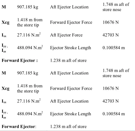
TABLE 2. Properties of the adjoining projectile and the separation mechanism.
M 907.185 kg Aft Ejector Location 1.748 m aft of store nose
Xcg 1.418 m from the store tip Forward Ejector Force 10676 N
Ixx 27.116 N.m2 Aft Ejector Force 42703 N
Iyy ,
Izz 488.094 N.m
2 Ejector Stroke Length 0.100584 m
Forward Ejector : 1.238 m aft of store
M 907.185 kg Aft Ejector Location 1.748 m aft of store nose
Xcg 1.418 m from the store tip Forward Ejector Force 10676 N
Ixx 27.116 N.m2 Aft Ejector Location 42703 N
Iyy ,
Izz 488.094 N.m
2 Ejector Stroke Length 0.100584 m
ForwardEjector: 1.238 m aft of store
After moving of boundary nodes as defined by the 6DOF trajectory, the secondary location of nodes will be obtained. In case the motion of the store is large, i.e. larger than that of adjacent cells, the smoothing method will be no longer valid. Therefore, the low-quality cells will be combined and locally remeshed based on the allowable skewness of the cells.
Due to the fact that an implicit algorithm has been used in the flow analysis, stability of the flow solver does not limit the duration of the time step Dt. However,
Dt in the time-dependent method is determined on the basis of precision and stability of the dynamic meshing algorithm, and thus it is limited to a certain value. Owing to complete adapting of the volume mesh, the so-called limit does not exist in the quasi-static method. Hence, the quasi-static method is preferable in this aspect. In this method, the program automatically uses the Gambit software for mesh generation in every time step, and modifies the volume mesh around the store after placing it in the new location.
7. VALIDATION AND CONTRAST
The separation simulation according to the wind tunnel test was performed in a Mach number of 1.2 in a 38000 ft altitude and a zero invasion angle. All other initial conditions are included in Table 1. Also, Table 2 includes the mass data as well as the separation force magnitudes and exertion points.
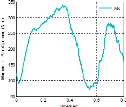
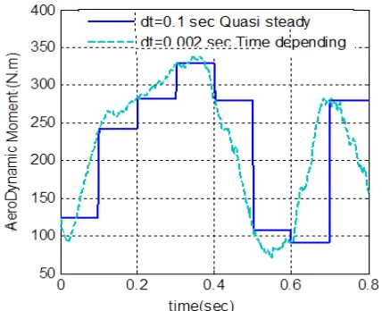
state of the store, using the time-dependent method, are shown in Figures 4 and 5. It can be observed that the graphs are in very good agreement with the wind tunnel test outcomes. Minor differences can be caused by neglecting viscosity or approximation in the separation mechanism modeling method. Figures 6 and 7 indicate the aerodynamic forces and moments exerted on the store’s mass center. Amid all, the moment around the longitudinal axis is more complicated due to its small magnitude and, at the same time, its large fluctuations with time, as more obviously observed in Figure 8. The mesh adapting method and pressure distribution in the symmetry plane before separation and after the 0.8 sec separation duration are shown in Figures 9 and 10, respectively. This reveals that the simulation works correctly. The alteration induced in the mesh around the store can also be noticed.
Figure 4. Center of gravity location (in the time-dependent method)
Figure 5. Angular orientation (in the time-dependent method)
Figure 6. Aerodynamic forces of the store vs. time
Figure 7. Aerodynamic moment in the store vs. time
Figure 9. Flow field meshing before separation and after the 0.8 sec duration in the symmetry plane (using the dynamic mesh method)
Figure 10. Center of gravity location, in the quasi-static method compared to the time-dependent method.
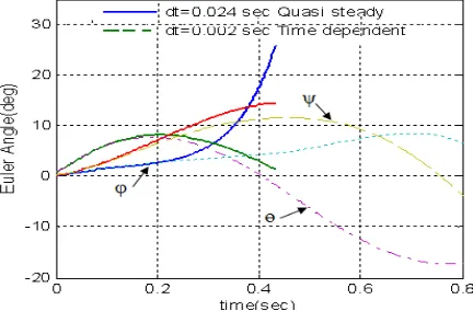
Figure 11. Angular orientation in the quasi-static method compared to the time-dependent method.
7. 2. The Quasi-static Method The quasi-static assumption is valid only in the first few instants of the separation procedure, i.e. until when the velocity of the store is not much larger than that of the flow velocity and the store is still close to the separation wing [4]. The variation in the position and state of the store using the quasi-static method are shown in Figures 10 and 11, respectively as compared to those obtained from the time-dependent method. It can be observed that the quasi-static solution diverges after 0.25 sec. Figure 9 demonstrates that the displacement has fewer errors, lying in the fact that other external forces, including gravity and separation mechanism, are more prevalent than aerodynamic forces.
7. 3. Reduction of the Solution Cost (Time) Two determinative factors, precision and cost (solution time) have been regarded in the present separation method. While the time-dependent method is more precise and reliable, it entails much calculation time, i.e. cost. Hence, it is not appropriate and proper for the separation system initial design. Although the quasi-static solution is very fast, it is unable to simulate realistically for not satisfying the problem conditions due to solution divergence as the store speed increases. Thus, the present research mainly aims at presenting a method to decrease the calculation cost while limiting the solution error within a specific range. The time step in this way can be enlarged, the solution can be carried out with fewer intermediate points, and the solution can be significantly faster with a limited error magnitude.
The traditional way to exert the aerodynamic forces is establishing a table of aerodynamic parameters based on the main factors of influence including the Mach number, invasion angle, relative positions or angles, etc., and using these parameters in the dynamic solution in the proper time intervals. Actually, due to the large number of data and parameters, it takes rather a long time to provide and update these tables, espcially for systems without a specified final geometry. Therefore, both time-dependent and quasi-static methods have been used automatically in the present research in the way that the mesh is refined in each time step based on the position change, and new aerodynamic forces will be obtained accordingly.
On the other hand, by enlarging the time step interval to the extent that the solution error remains in the prescribed limit, e.g. smaller than 30%, the solution speed will significantly increase. Owing to the fact that the implicit algorithm is used in the time-dependent method, stability of the solver does not constrain the time stepDt. Rather, Dt is determined based on the precision and stability of the dynamic meshing algorithm, and thus it is limited to a specified value [1]. However, the quasi-static method is independent of time step, and enlarging the time step will increase the error because of refining the volumetric mesh.
Thus, the quasi-static method is only useful for initial design calculations and will diverge soon after the beginning of separation. For instance, according to Figures 13-15, the rolling moment, and thus the angular velocity and the rate of the angular velocity are diverged after 0.2 seconds, and are hence no longer valid.
Figure 12. Aerodynamic roll moment exerted on the store
Figure 13. aerodynamic roll moment of the store.
Figure 14. Angular roll rate of the store
Figure 15. Variation of the roll angle of the store
8. RESULTS AND DISCUSSION
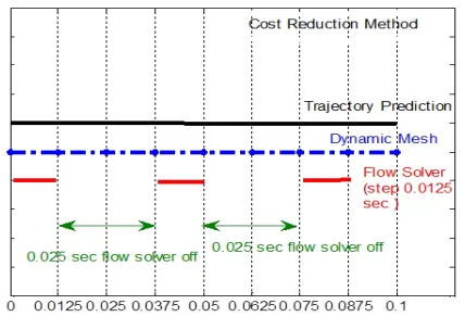
8. 1. Presentation of the Cost Reduction Scheme Using Dynamic Meshing in the Time-dependent Method As previously pointed out, the time step, in both the time-dependent and the quasi-static methods, cannot be enlarged due to divergence, even in the case of allowing the simulation error. Following is the presented method, intending to reduce the calculation time while allowing a specific solution error magnitude. In this way, the solution will be performed with far more rapidity. As stated earlier, the simulation procedure in each time increment consists of the flow solving, the 6-DOF trajectory, and meshing the field. Therefore, the total solution time needed for solution can be determined as:
Total Cost= Cost_ flow solving + Cost_ mesh update
+ Cost_ 6dof dynamic trajectory (5)
Total Cost= Cost_ flow solving + Cost_ mesh update (6)
As the only constraining factor limiting the time step in the time-dependent method is the remeshing algorithm rather than the flow solver, and since these two factors act independently, it will be convenient to refine the mesh in a time step without solving the flow. Namely, the program can freeze an intermediate time step and skip one solution round.
For instance, assuming that the total simulation duration is 0.8 sec and the time step is considered 0.0125 sec (the maximum allowable), then 64 solution steps (rounds) will be needed. If, in this case, the calculation of the flow is skipped in every other round, then 32 time steps will be skipped without divergence in the solution.
Therefore, if, the time for every solution round is supposedly 3.5 minutes, the 320-minute total time will be reduced by 112 minutes. Moreover, the total time can be further reduced by, for example, freezing every two other steps. Obviously, this will increase the error magnitude.
Figure 17, similar to Figure 15, indicates the variation in the rolling angle in both time-dependent and quasi-static methods. It can be easily observed that the solution will no more diverge, whereas the quasi-static method diverges after 0.3 seconds. Figure 18 shows the variation in the rolling angle vs. time, solved by skipping steps.
The same diagram for the moments 0.1, 0.2, and 0.3 sec, is shown in Figure 19. Figure 19 shows the total time reduction against the error magnitude. For instance, in the case that the time step is 0.0125 sec, this method reduces the total time by 38% and produces only 7.9% error. Finally, Figure 20 depicts the total solution time vs. the error magnitude for each method. In this figure, 0.0125 sec and 0.025 sec time steps have been basically used and the solution has been performed in every other step.
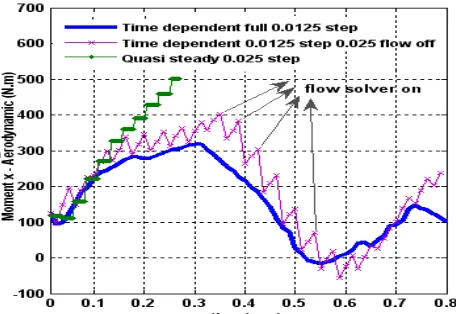
This figure reveals that the 0.025 sec time step with every other step solution skip, with a total solution time of 130 minutes, can prove efficacious to calculate the aerodynamic forces and moments since it entails only 17% error. Larger time steps can lead to greater errors (as 80% for a 0.05 sec time step) or unstable solutions. The variation of the aerodynamic moment around the x axis for the three methods including the direct time-dependent, the lower-cost time-time-dependent, and the quasi-static method is shown in Figure 21. It demonstrates that the low-cost time-dependent diagram satisfactorily agrees with the direct time-dependent diagram while the quasi-static diagram diverges quickly.
Figure 16. The cost reduction method proposed in the present research.
Figure 17. Variation of the rolling angle in the three solution methods.
Figure 19. The cost (time) reduction vs. error percentage.
Figure 20. The total solution time against the error percentage in each method
Figure 21. Aerodynamic moment exerted on the store around the x axis in the three methods.
Figure 22. Pressure distribution before and after the 0.8 sec separation duration
The reason behind convergence in the low-cost method is using dynamic meshing. Stated another way, when the flow solver calculates the values of compressive and shear stresses existing in mesh cells in each time step and skips solution in some following time steps, the dynamic meshing updates these stresses (by interpolating) simultaneously with mesh refinement. In this way, the properties of the present mesh are properly in accordance with the motion physical status, transferred into the following updated mesh. Meanwhile, effects due to velocity increase and disorder in the quasi-static state are resolved.
9. CONCLUSION
separation system due to its high cost. Because of not satisfying the problem conditions due to solution divergence with velocity, the quasi-static solution was, however, unable to simulate correctly even though it is very fast. The method presented in this work was able to reduce the calculation time while limiting the solution error within a specific allowable interval. Thus, the time step can be enlarged, the solution can be carried out with fewer points, and carried out far more rapidity within a limited error magnitude. As declared in the paper (Figure 20), the present method, can reduces the simulation time (cost) about 60% (210 min of 340 min), with acceptance of a 16% calculation error.
10. REFERENCES
1. Snyder, D. O., Koutsavdis, E. K. and Anttonen, J. S., "Transonic store separation using unstructured CFD with dynamic meshing", AIAA Paper, Vol. 3919, (2003).
2. PARESH PARIKH, V., SHAHYAR PIRZADEH, V. and NEAL, F., "Unstructured grid solutions to a wing/pylon/store configuration using VGRID3D/USM3D", (1992).
3. Meakin, R. L., "Computations of the unsteady flow about a generic wing/pylon/finned-store configuration", AIAA Paper, Vol. 4568, (1992).
4. Buning, P. G., Wong, T.-C., Dilley, A. D. and Pao, J. L., "Computational fluid dynamics prediction of hyper-x stage separation aerodynamics", Journal of Spacecraft and Rockets, Vol. 38, No. 6, (2001), 820-827.
5. Demir, H. o., "Computational fluid dynamics analysis of store separation", The Middle East Technical Univercity, Turkey, MSC Thesis, (2004),
6. Murman, S. M., Aftosmis, M. J. and Berger, M. J., "Simulations of 6-DOF motion with a Cartesian method", AIAA Paper, Vol. 1246, (2003), 2003.
7. Benmeddour, A., Fortin, F. and Jones, D., "Validation of a Quasi-Steady Euler Approach for Store Separation Using Unstructured Tetrahedral Meshes", in Proceedings of the CASI 7th Aerodynamics Symposium. (1999), 2-5.
8. Fortin, F., Benmeddour, A. and Tahi, A., "IAR stores clearance CFD approach: From development to automated engineering tool", ICAS 2002, (2002).
9. Ko, S.-H. and Kim, C., "Separation Motion of Strap-On Boosters with Base Flow and Turbulence Effects", Journal of Spacecraft and Rockets, Vol. 45, No. 3, (2008), 485-494. 10. Heim, E., "CFD wing/pylon/finned store mutual interference
wind tunnel experiment"., DTIC Document. (1991)
11. LOTH, E., Kailasanath, K. and Löhner, R., "Supersonic flow over an axisymmetric backward-facing step", Journal of Spacecraft and Rockets, Vol. 29, No. 3, (1992), 352-359. 12. Kirn, S., Mathur, S., Murthy, J., Choudhury, D. and Lebanon,
N., "A Reynolds-averaged Navier-Stokes solver using unstructured mesh-based finite-volume scheme", (1997).
Simulation of Store Separation using Low-cost CFD with Dynamic Meshing
M. Jafari a, A. Toloeia, S. Ghasemlu b, H. Parhizkar b
a Department of New Technologies Engineering, Shahid Beheshti University, Tehran, Iran b Department of Aerospace Engineering, Amirkabir University, Tehran, Iran
P A P E R I N F O
Paper history: Received 26 January 2013
Received in revised form 06 October 2013 Accepted 07 November 2013
Keywords: Store Separation Automatic Coupling Dynamic Mesh Quasi Static
Time Dependent Solution Low-cost CFD
هﺪﯿﮑﭼ
ﻪﯿﺒﺷ،ﻪﻟﺎﻘﻣﻦﯾارد زاهدﺎﻔﺘﺳاﺎﺑ،ﺎﻤﯿﭘاﻮﻫﮏﯾزاﺐﻤﺑﺶﯾاﺪﺟيزﺎﺳ
نﺎﯾﺮﺟﮏﯿﻣﺎﻨﯾدوﺮﯾآﺎﺑﮏﯿﻣﺎﻨﯾدتﻻدﺎﻌﻣﮏﯿﺗﺎﻣﻮﺗاﻞﭘﻮﮐ
ﻪﺘﻓﺮﮔراﺮﻗﯽﺳرﺮﺑدرﻮﻣﻢﺴﺟلﻮﺣ ﺖﺳا
.
لﺪﻣياﺮﺑ ﻪﺘﺴﺑاوشورودزاﮏﯿﻣﺎﻨﯾدوﺮﯾآيﺎﻫوﺮﯿﻧيزﺎﺳ ﻪﺑ
ﻪﮑﺒﺷﮏﻤﮐﻪﺑنﺎﻣز
ﻪﺒﺷﻞﺣوكﺮﺤﺘﻣ هﺪﺷهدﺎﻔﺘﺳاﺎﺘﺴﯾا
ﺖﺳا
.
ﻪﯿﺒﺷﻦﯾارد ﻪﻨﯾﺰﻫوﺖﻗدﻞﻣﺎﻋوديزﺎﺳ
)
نﺎﻣز
(
ﻪﺘﻓﺮﮔراﺮﻗﻪﺟﻮﺗدرﻮﻣﻞﺣ ﺪﻧا
.
دﺎﻤﺘﻋاﻞﺑﺎﻗوﻖﯿﻗدﯽﺷورنﺎﻣزﻪﺑﻪﺘﺴﺑاوﻞﺣﻪﮐﯽﻟﺎﺣرد ،ﺖﺳا
ًﺎﺘﺒﺴﻧﻪﻨﯾﺰﻫونﺎﻣزﯽﻟو ﯽﻣيدﺎﯾز
ﻞﯿﻟدﻦﯿﻤﻫﻪﺑوﺪﺒﻠﻃ
ﺳﺎﻨﻣﺶﯾاﺪﺟﻢﺘﺴﯿﺳﻪﯿﻟواﯽﺣاﺮﻃياﺮﺑ ﺖﺴﯿﻧﺐ
.
ﻪﺒﺷﻞﺣ ﺎﺘﺴﯾا ا ًﺎﺘﺒﺴﻧﺖﻋﺮﺳﻪﭼﺮﮔ درادﯽﯾﻻﺎﺑ
، ﻞﯿﻟدﻪﺑﯽﻟو ندﻮﺒﻧﺖﺳرد
ﻪﯿﺒﺷﻪﺑردﺎﻗ،ﻞﺣنﺪﺷاﺮﮔاووهﺪﺷاﺪﺟﺐﻤﺑﻦﺘﻓﺮﮔﺖﻋﺮﺳﺎﺑنآﻂﯾاﺮﺷ ﯽﻤﻧﻪﻠﺌﺴﻣيزﺎﺳ
ﺪﺷﺎﺑ
.
ﻪﯿﺒﺷرد يزﺎﺳ ،ﺮﺿﺎﺣ
ﻪﺘﺴﺑاوﻞﺣﻪﻨﯾﺰﻫونﺎﻣزﺶﻫﺎﮐياﺮﺑﯽﺷور ﻪﺑ
هﺪﺷﻪﺋارانﺎﻣز ﺖﺳا
ﻗﺶﻫﺎﮐﻦﯿﻋ ردﻪﮐ يﺎﻄﺧ،ﻞﺣنﺎﻣز ﻪﺟﻮﺗﻞﺑﺎ
هدوﺪﺤﻣردارتﺎﺒﺳﺎﺤﻣ ﮕﻧﯽﻗﺎﺑهﺪﺷﻦﯿﯿﻌﺗولﻮﺒﻗﻞﺑﺎﻗي
ﺎه ﯽﻣ دراد
.
ﯽﻣرﺎﮐﻦﯾاﺎﺑ ردﺎﻬﻨﺗ،ﯽﻧﺎﻣزمﺎﮔراﺪﻘﻣﺶﯾاﺰﻓاﺎﺑ ناﻮﺗ
راﺪﻘﻣلﻮﺒﻗﺎﺑوﺖﺧادﺮﭘنﺎﯾﺮﺟﻞﺣﻪﺑ،دوﺪﺤﻣﻪﻄﻘﻧﺪﻨﭼ ارﻞﺣﺖﻋﺮﺳ،ﺎﻄﺧﯽﺼﺨﺸﻣ
ﻪﺑ ﺑﺪﻨﭼ ﺮا ﺑ ﺮ ﺶﯾاﺰﻓا داد . ﻦﯾارد
ﻪﺑ ﻪﻟﺎﻘﻣ ﯽﺘﺳاررﻮﻈﻨﻣ مﺮﻧﯽﯾﺎﻣزآ
ﺮﻓ،رﻮﮐﺬﻣراﺰﻓا ا
ﻢﺴﺟﺶﯾاﺪﺟﺪﻨﯾ هﺮﮑﯿﭘﮏﯾزاﯽﻗﺎﺤﻟا
لﺎﺑيﺪﻨﺑ -نﻮﻠﯾﺎﭘ -ﻢﺴﺟ ردﯽﻗﺎﺤﻟا
نﺎﯿﻣيزاوﺮﭘﻂﯾاﺮﺷ ﻪﯿﺒﺷﯽﺗﻮﺻ
هﺪﺷيزﺎﺳ ﺖﺳا ﺖﻗدﺮﮕﻧﺎﯿﺑ،دﺎﺑﻞﻧﻮﺗﺖﺴﺗﺞﯾﺎﺘﻧﺎﺑنآﺞﯾﺎﺘﻧﻪﺴﯾﺎﻘﻣﻪﮐ ﯽﻣنآﺐﺳﺎﻨﻣ