Optimization of Heat Transfer Enhancement of a Domestic Gas Burner Based on Pareto Genetic Algorithm: Experimental and Numerical Approach

International Journal of Engineering

J o u r n a l H o m e p a g e : w w w . i j e . i r

Optimization of Heat Transfer Enhancement of a Domestic Gas Burner Based on

Pareto Genetic Algorithm: Experimental and Numerical Approach

G. Ghassabi*, M. Kahrom

Department of Mechanical Engineering, Ferdowsi University of Mashhad, Mashhad, Iran

P A P E R I N F O

Paper history: Received 30 August 2012

Received in revised form 2 November 2012 Accepted 15 November 2012

Keywords: Pareto Front

Heat Transfer Efficiency Skin Friction Reynolds Analogy Probability Density Function

A B S T R A C T

The present study attempts to improve heat transfer efficiency of a domestic gas burner by enhancing heat transfer from flue gases. Heat transfer can be augmented using the obstacles that are inserted into the flow field near the the heated wall of the domsetic gas burner. First, to achive the maximum efficiency, the insert geometry is optimized by the multi-objective genetic algorithm, so that heat transfer is maximized while minimizing the skin frication. Then, the heating unit is modeled as a three dimensional physical domain. The conservation equations of mass, momentum, energy and species are discretized over the meshing system of control volumes in the domain. The experimental set-up is equally established to measure and validate the numerical results. The effect of the inserts on heat transfer enhancement is studied both numerically and experimentally. The results show that the optimal insert is a triangle with the scaled area of 12.4 mm2_{. Also, the results indicate that the}

optimal inserts led to the improvement of heat transfer efficiency by 2.7% compared with the case of similar environment with no insert.

doi:10.5829/idosi.ije.2013.26.01a.09

NOMENCLATURE

f Mixture fraction Greek Symbols

Gk Generation of turbulent kinetic energy due to the average velocity gradient ak,e Inverse effective prandtl number

Gb Generation of turbulent kinetic energy due to the buoyant forces gj Mass of the jth mass fraction component

hc Heat transfer coefficient meff Effective viscosity

H Total enthalpy _t Stress tensor

I Unit tensor Q Flow rate

1. INTRODUCTION1

Domestic burners share a significant amount of nonindustrial energy consumption. Most burners have a thermal efficiency of less than 30% [1]. Improving the heat transfer efficiency of a domestic gas burner is the main task of the present work. Exhausting hot gases are one of the most important reasons that reduce heat

* _{Corresponding Author Email: [email protected] (G.}

Ghassabi)

increases by increasing heat transfer. In the combustion chamber, augmentation of the skin friction avoids to exhaust combustion products. Therefore, in this situation, combustion is incomplete and decreases heat transfer efficiency. Other means of heat transfer enhancement is to insert an object into the turbulent boundary layer of the flow field, [4, 5]. By doing so, a stagnation point forms over the frontal area of the insert geometry, providing a driving force to push the flow stream from the gap between the obstacle and the wall. The jet passing through the gap is a cause of vortex generation at downstream to the obstacle which in turn, makes considerable contribution to the heat transfer enhancement as is experienced by Kahrom, et al. [6]. Inaoka, et al. [7] placed an insert into the turbulent boundary layer and measured both the heat and skin friction coefficients along the affected area. Amazingly, the results violated the Reynolds Analogy between heat and momentum transfer in that the insert was a cause of heat transfer enhancement (HTE), while the skin friction also happened to be reduced simultaneously. More studies by Teraguchi, et al. [8], Kahrom, et al. [9] and Kong, et al. [10] also reported the same type of violation of the Reynolds Analogy. Hence, placing an insert in the flow field is a good idea to improve heat transfer of a domestic gas burner and to decrease skin friction. Nonetheless, blockage effect by an insert decreases efficiency, since this effect avoids to exhaust combustion products and therefore combustion is incomplete. To access the maximum efficiency, this paper insists on finding a particular insert geometry which can provide the maximum heat transfer while minimizing skin friction and blockage effect by an obstacle. Thus, the problem is one of three objectives optimization. The optimization of multi-objective functions that are in conflict with each other is best handled by the multi-objective genetic algorithm. MacCormack, et al. [11] employed the Genetic algorithm (GA) to optimize suction distribution over a flat plate in order to delay transition and therefore reducing the friction drag. Leng, et al. [12] used GA to optimize the design of a small flying object and so achieved optimized lift and drag forces on the body. Amanifard, et al. [13] employed multi-objective GA and a neural network to optimize heat flux from a rectangular cylinder at Red=1400. The cylinder was placed at different distances from a flat plate and the effect of distances on the strouhal number and lift was studied. More application of GA on optimization of heat transfer devices are reported by Xie, et al. [14], Gholap, et al. [15], Amanifard, et al. [16] and Hilbert, et al. [17]. This paper aims to achieve two goals. First, as a new work, insert geometry is optimized by the multi-objective genetic algorithm; so that heat transfer is maximized while minimizing the skin friction and blockage effect. Second, the effect of optimal insert on heat transfer augmentation and, consequently, on heat

transfer efficiency of a domestic gas burner are investigated both numerically and experimentally.

2. NUMERICAL TECHNIQUE AND GOVERNING EQUATIONS

The turbulent mixing flow of air and burning gases, the combustion process and natural convection throughout the computational domain is simulated by solving the continuity, momentum and energy equations over the physical domain. The general form of continuity equation: (1) m S ) v .( t +Ñ =

¶

¶r _rr

Sm is the mass added to the air phase from a secondary phase change and is ignored for gaseous type of fuels. The momentum equation reads as:

(2) g ) .( p ) v v .( ) v ( t r r r

r _{r t r}

r +Ñ =-Ñ +Ñ +

¶ ¶

In which the stress tensor,t, is defined as:

(3) ]

I . )

[( n nT n

m

t = Ñr+Ñr - Ñ r

3 2

To replace the components of stress tensor, we apply RNG k-e turbulence model. In which the transport equations for the k and

e

(4)

( ) ( i) ( k eff ) k b

i j j

k

k k u G G

t r x r x a m x re

¶ ₊ ¶ ₌ ¶ ¶ _{+ +} -¶ ¶ ¶ ¶ (5) 1 3 2 2

( ) ( i) ( eff ) ( k b)

i j j

u C G C G

t x x x k

C R

k

e e e

e e

e e

re re a m

e r

¶ ₊ ¶ ₌ ¶ ¶ _{+ +}

¶ ¶ ¶ ¶

-

-In Equation (5), C_1e and C_2eare equal 1.42 and 1.68, respectively. Gk, the generation of turbulent kinetic energy due to the average velocity gradient and Gb, the generation of turbulence kinetic energy due to buoyant forces, m_eff, effective viscosity, a_k and a_e, inverse effective prandtl numbers are replaced by:

(6) i j j i k x u u u G ¶ ¶ ¢ ¢ -= r (7) i t t i b x T Pr g G ¶ ¶

=b m

(8) eff . . . . . . m m a a a a ₌ + + -- 6321 0 6321

0 23929

3929 2 3929 1 3929 1

In which, a₀ is 1.0. By assuming non adiabatic combustion, the partial mixture implementation is impressed as terms of enthalpy in the energy equation:

(9)

h p

t _{H) S}

c k .( ) H v .( ) H (

t +Ñ =Ñ Ñ +

¶

In which Kt presents the turbulent conduction heat transfer. Here, the enthalpy is defined as:

(10)

j jh

H=

å

where, g_j is the mass of the jth mass fraction component in the total mass of flue gases for which the enthalpy is defined as:

(11) ) T ( h dT c

H ref,j

T T j j , p j ref

ò

The h_j0(T_ref,j) is the enthalpy of the jth portion of the

gas at a reference temperature of T_ref,j. The source term in Equation (9) for a chemical reaction is explained as: (12) j i j j h R M h S =-

å

0

In the energy equation, the enthalpy, states the energy devoted to the formation of each type of combustion products. The combustion is assumed to perform in atmospheric pressure and the situation involves high density fluctuation in the flow stream. The combustion also involves the intermediate combustion products such as H2 and CO and the temperature distribution and chemical reactions consider together. Thus, the probability density function, namely the PDF approximation is employed. The PDF method has the advantage of predicting many of intermediate reaction products. Such as we did in present work, the concentration for 7 probable combustion products including the CH4, O2, CO2, CO, H2O, H2 and N2 are assumed and calculated. Transport equations for mixture fraction (f ), its variance (_f¢2_{) and (h) are} solved. In systems with heat transfer, in which the change in enthalpy affects the mixing process, the thermo-chemical situation of mixture is not assumed to be a temporal enthalpy. However, the calculation of the temporal enthalpy in engineering applications is uneconomical and here is ignored. The reason is that the fluctuation encounters with enthalpy is independent of enthalpy itself. Putting these all together, the effect of fluctuation on thermo-chemical reaction, considering the specific function is:

(13) df ) f ( P ) H , f ( i i=

ò

1

0 f f

A function, P(f ), is employed to relate the time averaged of mass fraction of species to the temperature and fluctuation of mixture fraction. The density distribution function as a function of averaged fraction of mixture and its variance is defined as:

(14) 1 0 1 1 1 1 0 1 1 1 < < -= -ò f , df ) f ( f ) f ( f ) f ( P b a b a In which: (15) 1] f ) f (1 f [ f α 2 -¢ -= 1] f ) f (1 f [ f) ( 2 -¢ -=1 b

Using averaging [18], the two variables fand _f¢2_in

each computational zone is calculated from conservation equations: (16) ) x f ( x ) f u (

x t i

t i i i ¶ ¶ ¶ ¶ = ¶ ¶ s m r (17) 2 2 2 2

( ) ( t )

i g t

i j t j i

d

f f

u f C

x x x x

C f k m r m s e r æ ö ¢ ¶ _{¢ =} ¶ ¶ ₊ ¶ ç ÷

¶ ¶ ¶ _è¶ _ø

¢

-The constants s_t, Cg(=2/st) and Cdare 0.7, 2.86 and 2.0, respectively.

3. OPTIMIZATION OF INSERT GEOMETRY BY GA

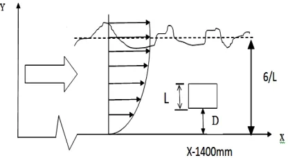
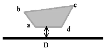
3. 1. Problem Deinition As shown in Figure 1, air flows at 20 O C parallel to a flat plate which is at a constant surface temperature of 70 O C. At x=1400 mm from the leading edge, at which Re=1.63E6, a quad is inserted into the turbulent boundary layer. Depending on the quad shape and its distance from the flat plate, the deformation of the boundary layer is specified, thus creating a specific distribution of the heat and friction coefficients over the flat plate for each configuration. A sample shape of a quad at the vicinity of a flat plate is presented in Figure 2. By optimization, the coordinates of four corners a, b, c and d of the quad are changed until the optimal group of shapes and their distances (D) from the flat plate is reached. To facilitate the comparison between many different cases of studies, an affected areais defined as the area of the flat plate on which the local heat transfer coefficient is stimulated by

±

Figure 2. A sample quad located in a turbulent boundary layer of a flat plate

3. 2. Multi-Objective Genetic Algorithm GA is based on an analogy with the evolution theory, i.e. the inevitable course of nature. Alike in nature, an original population of individuals is manually created and represents a primitive generation of parents. Each individual's fitness is first determined by how well that individual adapts to a given environment and then evaluated by how well that individual survives. Fit individuals go through a process of survival solution, crossover and mutation which results in the creation of the next generation of individuals, indeed the children individuals.

Who are formed from a selection of optimum individuals that is parents and children. Since solution algorithms are relatively different for GAs, it is important to distinguish between single-objective and multi-objective GAs. In multi-objective GAs, as is in this study, the aim is to find many non-dominated solutions, whose performance spreads over the objective functions domain, known as the Paretofront. According to Pareto's rule, the individual A dominates the individual B if, for at least one of the objectives, A is clearly better adapted than B and if, for all other objectives, A is no worse than B. An objective is considered optimal if it is non-dominated in the sense of this rule. To each of the individuals, a rank number is devoted that is equal to the number of individuals dominating it. If an individual is not dominated by any other, it is given the top ranking number, the numeral one. An individual i which is dominated by j individuals receives the rank i=j+1. Non-dominated individuals always have a rank of one. At the end, the best individuals are all the non-dominated individuals throughout all generations, leading to what is called the Pareto front. This rule classifies the individuals of the population to calculate the corresponding fitness values [17]. In each step of the solution, the objective vector y

is called the Pareto-optimal if and only if there is no feasible solution that dominates this solution vector. These Pareto-optionalsolutions form the Pareto front.

3. 3. Multi-Objective Variables To formulate the problem, a vector variable x is considered as genes in:.

X ) x ,... x , x (

x= _{1 2 n} Î (18)

When applying the vector function f

) f , f , f (

f = _{1 2 3} (19)

X maps onto an objective vector Y as:

Y ) y ,... y , y (

y= 1 2 n Î (20)

More specifically for the present case, the elements of vector x are coordinates of four varying vertices of the quad, namely vertices a, b, c and d of the quad as are shown in the Figure 2.

1 8

(x ,...,xi...x )=(xa,ya,xb,yb,xc,yc,xd,yd) (21)

To calculate the local heat transfer coefficients there is:

.)]} y )( T T /[( ) T T {( k h y ) T T ( k A Q ) T T ( h A Q i W i W cx i i W W cx 0 0 2 2 2 2 -= -= -= = ¥ = = = ¥ (22)

in which, y i is the distance of the second grid from the wall of the quad or the flat plate, and similarly so for the friction coefficient 2 2 2 [ ] / ( ) 0 2 i

w f x w

i

u U

C y

r

t m = t ¥

=

= ® =

- (23)

Finally, the averaged heat and friction coefficients over the affected area are:

) x ( f

h_c= ₁ ,

_ò

D = 2 1 1 l l cx

c h dx

x h (24) And: ) x ( f

C_f = ₂ ,

_ò

D = 2 1 1 l l fx

f C dx

x

C (25)

The area of the quad is responsible for the flow blockage and has to be minimized in this optimization:

)]} y y ( x ) y y ( x ) y y ( x [ { )]} y y ( x ) y y ( x ) y y ( x [ { A ) x ( f A c a d a d c d c a b a c a c b c b a -+ -+ -+ -+ -+ -= = 2 1 2 1 3 (26)

Values of hc, Cf and A are components of the objective vector, y=(y1,y2,y3). Constraint must be exercised to keep variables within reasonable ranges.

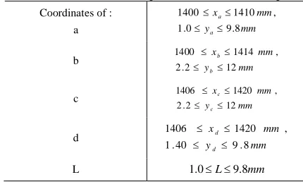
defined ranges. Table 1 shows limitations to keep the quad inside the boundary layer and in a position where

Rex remains constant as specified before. Here, coordinates of four vertices are the basic elements of the constraint vector. Numerically, these are specified in Table 2. Other variables, ui=2 and Ti=2, are consequences of solutions of flow equations around the newly formed quad.

By imposing these constraints, quad edges remain within agreed physical ranges:

In all cases of examination, the whole body of the quad remains inside the boundary layer. One of the edges of the quad is always kept parallel to the flat plate. None of edges is eliminated in optimization. GA, in its first step, assumes a primitive population (NPOP), which is formed by using arbitrary design variables in the permitted range of values. Each set of adopted variables defines a member of a generation. In the next step, based on the results for the first generation's objective vector, the same technique is employed to assign populations for the next generation. The following are parameters defining the decision making: Population size, Generation, Crossover probability, Mutation probability, Selection strategy.

TABLE 1. Limitations imposed on vertices of the quad

Coordinates of :

a y mm

mm x

a a

8 . 9 0 . 1

, 1410 1400

£ £

£ £

b

mm y

mm x

b b

12 2 . 2

, 1414 1400

£ £

£ £

c

mm y

mm x

c c

12 2 . 2

, 1420 1406

£ £

£ £

d

mm y

mm x

d d

8 . 9 40

. 1

, 1420 1406

£ £

£ £

L 1.0£L£9.8mm

TABLE 2. Constraints imposed to quad coordinates

1 xapxd

2 xbpxc

3 y_apy_b, y_apy_c

4 ya=yd

In crossover, genes are selected from either one of the parents or are mixed randomly in a crossover process. In this way, randomly selected genes from both parents will be kept for the future generations. By

averaging or crossover, mutation operator then modifies individual genes to obtain the next generation individuals. Once a population is initiated, it is sorted based on domination reasoning; the first front is completely non-dominated in the current population and the second front (the next generation) is dominating individuals of the first front, and so on. An algorithm decides how to choose transcendence members from the present generation to motivate the next generation. The odds assigned to each member to advance to next generation are:

å

=

popsize

i i

i i

f f p

1

(27)

where, fi is the transcendence of the ith member in the generation. The production of each member of a generation is assumed to be a function of the crossover probability PC and the mutation probability function Pm. The size of the population must be large enough to achieve a better selection in shorter sequences. However, by increasing the number of the population, the amount of calculation increases and so lowers the rate of convergence. Since the selection strategy is based on probability, there is no guarantee of arriving at a better combination of population in the next generation. There is also a chance of diverging from the optimized target [19].

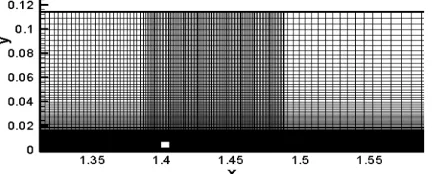
3. 5. Grid Generation and Code Verification Grid point distribution in a computational domain is non-uniform. Unlike a single flow field examination that is the subject of much research work, the present work is comprised of 1,600 different compositions of a quad and a flat plate boundary layer that must be re-meshed and resolved sequentially. It is difficult to address a precise mesh organization. Here, to achieve the best use of turbulence models, the laminar sublayer must be touched by the model in other words, at least one grid point must be located inside the sub-layer. Therefore, the strategy in each remeshing is to locate the first grid point on the solid walls, along with the flat plate and surfaces of the quad. Then, the next grid point is located at a distance of not more than y2+ - y1+

f

on the flat plate and surfaces of the quad. The height of flow over the flat plate is chosen so that it is large enough to minimize the influence of flow blockage due to growth and disturbances imposed by the boundary layer.

To assure the validity of the present numerical code, hot wire anemometry is performed in a wind tunnel. A similar flow condition, as described in section 3-1, is imposed. A square rod, with a cross section of 8 mm*8 mm, is placed at a distance D = 8 mm from the flat plate, inside the turbulent boundary layer of the flat plate where Re=1.63E06. The average velocity profile at downstream to the rod is measured by hotwire [20]. The comparison between the solution of the present code and measurements at a distance of x/c=5/8 is presented in Figure 4. X is the distance from the rear stagnation point and c is the length of the quad. As the figure shows, strong agreement exists between the experimental and numerical solutions. The figure compares solutions for three cases of mesh generations with a stretching factor of s=1.08 (grids 410*167), s = 1.1 (grids 390*155), and s = 1.12 (grids 370*140). Optimum agreement at s=1.08 is reached and the meshing strategy accepted being employed throughout the present study.

Figure 3. Sample meshing for a rectangular near a flat plate

Figure 4. Comparison of mean velocity profiles with measured data

3. 6.Results The process of optimization is initiated by random creation of the first twenty individuals making up for the first generation. Each individual represents a quad shape and its distance from the flat plate is as explained in section 3.4. For each individual, the meshing strategy is applied, then the flow equations are solved and the variation of the local heat transfer coefficient and skin friction is met. Beginning with random creation of the initial population of the first generation, in the range of design variables of Table 1, the algorithm iteratively produces a sequence of new generations until the criterion for halting this sequence, the 80th generation, is encountered. During the process, the selection of parents is based on their fitness; children (or the population of the next generation) are created by making random changes to a single parent (mutation) or by combining the vector entries of a pair of parents (crossover) and then replacing the current population with the next generation. The algorithm selects the most fit to form the next generation. This technique guarantees the algorithm's approach to choosing the best individuals for the last generation. Twenty individuals from the last generation are considered the best quads when compared to all individuals of previous generations. This results in

optimum heat transfer enhancement while

Figure 5.Three-dimensional presentation of objective vector components plotted as the Paretocurve

Figure 6. Averaged flow field around the triangular geometry of the pareto front

4. THE EFFECT OF OPTIMAL INSERT ON HEAT TRANSFER ENHANCEMENT OF A DOMESTIC GAS BURNER

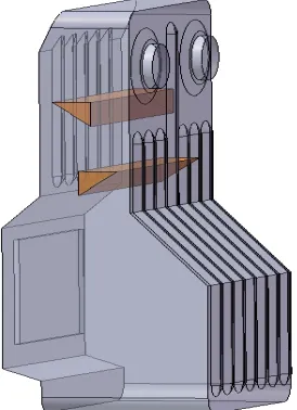
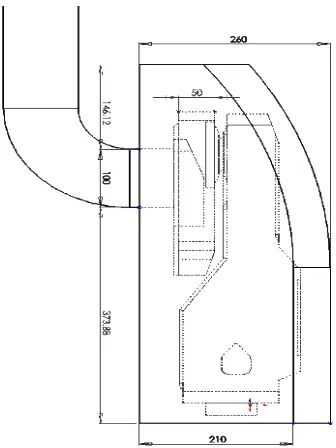
Considering the results of the previous section, to examine the effect of optimal insert on heat transfer enhancement of a domestic gas burner and its efficiency, two triangular bars were imposed on the flow field near the heated wall at the entry and midway of the upper chamber. By experience, the placement of inserts was chosen to result in less flow pressure losses as well as total flow rate. In Figure 7, placement of both triangular bars, as inserts, are shown. Figure 8 shows the internal body and placement position of inserts. Figures 9 and 10 show dimensional details of heating system.

Figure 7. Right triangular bars are located inside the heating unit

(a)befor assembling (b)after assembling

Figure 8. The internal body and placement position of inserts

Figure 10. Details of configurations and dimensional details

TABLE 3. Specifications of testo 325M

Accuracy Range of

measurement case

±0.4°C 0- 200°C

Temperature (0C)

±1.0°C 200- 900°C

0.2%± 0-25%

O2 (%)

10 ppm± 0-10000 ppm

CO (ppm)

8 ppm± 0-3000 ppm

NO(ppm)

0.1% ---

Excess air (%)

4. 1. The Experimental Setup One of the widely used commercial domestic heating units with 6000 kcal/hr gas burning capacity was selected for experimental measurements. The combustion chamber and settling chamber were connected by a 96 mm pipe. Methane gas was entered through a nozzle into the burner while dragging some of the surrounding air. The air was mixed with the methane before reaching the burning point. As a result of burning, the temperature of the flowing gases was raised and the resulting buoyant force drove the combustion products towards the exhaust. As the air and the methane entered into the combustion chamber and burning process was completed, hot gases moved through the two pipes into the settlement zone. By entering the combustion products into the chimney entrance, the buoyant force helped to extract gases to the free air. Depending on the value of the imposed buoyant force, extra air was

sucked into the furnace in which it was later mixed by the combustion products and was lifted towards the chimney. A domestic gas burner was borrowed from the manufacturer. The gas meter, an in-touch thermometer probe (testo 925) and (testo 325M) a gas analyzer were used as the measurement devices. These devices were first calibrated according to the standard probe suggested by the provider. The temperature of the external surfaces and accessible points of the combustion chamber were specified by testo 925. Temperature of the chimney and concentration of combustion products were measured at burner exhaust using testo 325M. The standard probe of testo 325M can measure temperatures up to 1000°C by a k type thermocouple. This device directly estimates the concentration of O2, CO and NO. However, concentration of CO2 was measured using percentage of the measured concentration of O2. In Table 3, the calibrated sensor specifications of testo 325M is represented. Recurrent point-by-point measurements were performed every 15 minutes at each point until reaching less than about 5% difference in the change of two successive measurements at each point compared with its previously measured value. Then, the state was assumed to be stable. The experiments were performed for Qgas =7 liters/min of methane gas flow rate.

4. 2. Mesh Generation and Boundary Conditions

rest of the coming air was entered from the opening in the back side of furnace. For such boundaries, exhausting gases to chimney and upper plane of the combustion chamber, the pressure outlet boundary condition was used. The mass fraction of oxygen and nitrogen for these boundaries were assumed 0.23 and 0.77, respectively. Figure 11 shows meshing in physical domain and boundary conditions for the domestic heating unit. The laboratory's air temperature was 25 0C during the experiment. The outer body was exposed to the free room air flow and provided heat transfer by free convection to the outside air. For the calculation of this heat transfer coefficient, average outer wall temperature of heating unit was considered 100 0C. For the calculation of Rayleigh number, the film temperature was 335.5 K and the heat transfer surface height was 62 cm.

At the end of numerical calculation and also temperature measurements over the heating device, the following measures were concluded:

8 10 9

3 ´

= .

Ra_body (28)

Which means the external body heat transfer is of laminar nature. The Nusselt number reads [21]:

(Pr) g Gr Nu

/ L L

4 1

4 3 4

÷ ø ö ç è æ

= (29)

in which:

4 1 2

1 2 1

238 1 221 1 609 0

75 0

/ /

/

Pr) . Pr . . (

Pr . (Pr)

g

+ +

= ₍₃₀₎

The physical properties were counted at film temperature ending with g(Pr)=0.5 and NuL=89.94 which resulted in h =4.05W /m2K

Figure 11. Meshing in physical domain

4. 3. Results and Discussion In Table 4, a comparison is demonstrated between the numerical prediction of combustion products and experimental data for a case with no insert at the exhaust. It can be seen that the percentage of carbon monoxide is very low. Furthermore, unlike the obvious numerical error on CO products at the exhaust, other components are in agreement with the experiments. One may suggest that the premixing assumption for the air and fuel would be the cause of the encountered error.

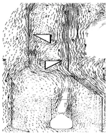
Figure 13 displays velocity vectors of exhaust gases in two planes of the heating unit, as shown in Figure 12. According to the figure, by inserts, the flow conducted towards the wall, providing a strong jet over the chamber walls. The numerical solution shows the flow disturbances and unveils the flow behavior near the wall.

TABLE 4. Comparison between the numerical prediction of combustion products and experimental data for a case with no insert at the exhaust

Numerical simulation Experimental

407 392

Temperature (K)

Less than 1.0 11

CO (ppm)

16.3 16.5

O2 (%)

2.59 2.6

CO2 (%)

Figure 12. Two planes of the heating unit

Plane 2

Figure 13. Velocity vectors of exhaust gases in tow planes of the heating unit (as shown in Figure 12)

Figure 14. Method of measuring wall temperature

To validate the numerical evaluation, temperature distribution over the external surface of the burner including the body, top surface of the combustion chamber and the passages between combustion chamber and settlement zone was measured and compared with the numerical results. Figure 14 presents the point and the method of measuring wall temperature using in-touch temperature probs. Figure 15 shows the experimental measurements of temperature on external surfaces of the combustion chamber. In the same figure, the numerics are the measured temperature and simultaneously the filled counter presents the numerical result. The results agree on the trend of temperature variation. However, the most deviation from the experiment is limited to about 6% in error. Figure 16 compares the same numerical and experimental case on the top wall and the joining pipes of the chamber. It observed that the numerical result has good agreement with the experimental data.

X

0 0.2 0.4 0.6

Y

-0.1 0

0.1 _-0.2 0Z

0.2

Temp. (K) 430 420 410 400 390 380 370 360 350 340 330 320 310

381 404

405 380

346.6

413 449

456 393

356.5

393 422

419 374

347

Figure 15. Comparison of numerical simulation results with the experimental data on external surfaces of the combustion chamber (the numerics are the measured temperature and the filled counters are the numerical results)

s

Temp. (K) 520 500 490 480 460 450 440 420 400 380 360 340 320

455 467 461

478 490 479

553 543

488 515 523

517 497

Figure 16. The comparison numerical simulation results with the experimental data on the top wall of the chamber

TABLE 5. Comparison between the numerical prediction of combustion products and experimental data for a case with insert at the exhaust

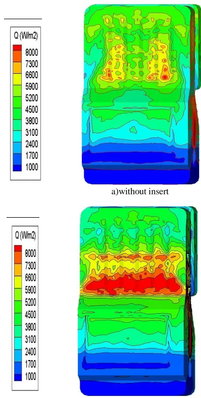
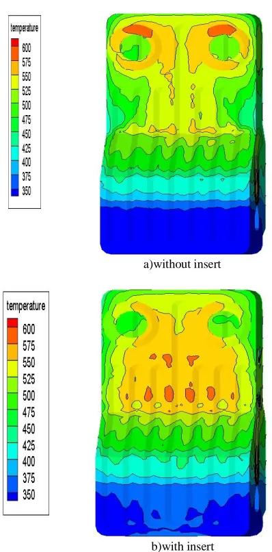
In Figure 17, temperature distribution over the chamber wall is compared for the two cases of with and without insert. The average wall temperature increases when the inserts are implemented. Figure 18 demonstrates the effect of inserts on the rate of heat release over the chamber wall. The heat is released to the wall in which the installed inserts clearly enhances by 16.24% and heat loss from chimney decreases by 7.8% (as shown by the measurements). Numerical evaluation shows 2.7% increase in heat transfer efficiency of the heating system. Here, efficiency defined as the heat released to the surrounding air divided by Lower Heat Value (LHV) of the burning gas. In Figure 19, temperature distribution over the wall behind the chamber is represented for the two cases of with and without insert. It can be seen that the temperature of the joining piping wall of the chamber decreases when the insert is implemented. This is due to the improvement in the rate of heat release over the wall chamber.

a)without insert

b)with insert

Figure 17. The effect of insert on the temperature distribution over the chamber wall

a)without insert

b)with insert

Figure 18. The effect of insert on the rate of heat release over the chamber wall

Numerical simulation Experimental

397 384

Temperature (K)

Less than 1.0 22

CO (ppm)

16.2 16.4

O2 (%)

2.65 2.54

a)without insert

b)with insert

Figure 19. The effect of insert on the temperature distribution over the wall behind the chamber

5. CONCLUSION

In this paper, the enhancement of heat transfer efficiency of a domestic gas burner was studied, both numerically and experimentally. For the enhancement of efficiency, the two inserts, optimized by GA, were placed into the flow field near the heated wall of the combustion chamber. The results were compared in the two cases of with and without insert. The following conclusions are reached from the analysis of results: 1. Based on pareto curve, the optimum insert was a

triangular obstacle with the scaled cross sectional area of 12.4 mm2.

2. When the optimum insert was implemented, high heat transfer rate to the chamber walls increased wall temperature and, in turn, caused 16.24% more heat transfer to the ambient air.

3. Heat transfer efficiency of a domestic gas burner increased by 2.7%.

4. The comparison showed that the numerical results were strongly in agreement with the experiments.

6. REFERENCES

1. Tajwar, S., Saleemi, A.R., Ramzan, N. and Naveed, S., “Improving thermal and combustion efficiency of gas water heater”, Applied Thermal Engineering, Vol. 31, (2011), 1305-1312.

2. Perry, L.Y., “Surface roughness effects on heat transfer in micro scale single phase”, Proceedings of the Sixth International ASME Conference on Nano channels,Micro channels and Mini channels, Darmstadt,Germany, 2008.

3. Suzue, Y., Morimoto, K., Shikazono, N., Suzuki, Y. and Kasagi, N., “High performance heat exchanger with oblique wavy walls”, 13th international Heat Transfer Conference, Sydney,Australia, 2006.

4. Shuja, S.Z., Yilbas, B.S., Iqbal, M.O. and Budair, M.O., “Flow through a protruding bluff body–heat and irreversibility analysis”, exergy, Vol. 1, (2001), 209–215.

5. Zhdanov, V.L. and Papenfuss, H.D., “Bluff body drag control by boundary layer disturbances”, Experiments in Fluids, Vol. 34, (2003), 460–466.

6. Kahrom, M., Farievar, S. and Haidarie, A., “The effect of square splittered and unsplittered rods in flat plate heat tansfer enhancement”, International Journal of Engineering, Vol. 20, (2007), 83-94.

7. Inaoka, J., Yamamoto, J. and Suzuki, K., “Dissimilarity between heat transfer and momentum transfer in a disturbed boundary layer with insertion of a rod modeling and numerical simulation”, International Journal of Heat and Fluid Flow, Vol. 20, (1999), 290-301.

8. Teraguchi, K., Katoh, K. and Azuma, T., “Dissimilarity between turbulent momentum and heat transfer by excitation of transverse vortex”, Journal of The Japan Society of Mechanical Engineers, Vol. 80, (2005).

9. Kahrom, M., Haghparast, P. and Javadi, S.M., “Optimization of heat transfer enhancement of a flat plate based on pareto genetic algorithm ”, International Journal of Engineering, Vol. 23, (2010), 177-190.

10. Kong, H., Choi, H. and Lee, J.S., “Dissimilarity between the velocity and temperature fields in a perturbed turbulent thermal boundary layer”, Physics Of Fluids, Vol. 13, (2001), 1466. 11. MacCormack, W., Tutty, O.R., Rogers, E. and Nelson, P.A.,

“Stochastic optimization based control of boundary layer transition”, Control Engineering Practice, Vol. 10, (2002), 243-260.

12. Leng, G.S.B. and Ng, T.T.H., “Application of genetic algorithms to conceptual design of a micro-air vehicle”, Engineering Applications of Artificial Intelligence, Vol. 15, (2002), 439– 445.

13. Amanifard, A., Nariman-Zadeh, N., Borji, M., Khlkhali, A. and Habibdoust, A., “Modeling and Pareto optimization of heat transfer and flow coefficients in micro channels using GMDH type neutral networks and genetic algorithms”, Journal of Energy Conversion and Management, Vol. 49, (2008), 311-325.

15. Gholap, A.K. and Khan, J.A., “Design and multi-objective optimization of heat exchangers for refrigerators”, Journal of Applied Energy, Vol. 84, (2007), 1226– 1239.

16. Amanifard, N., Hajiloo, A. and Tohidi, N., “Using neural networks and genetic algorithms for modeling and multi-objective optimal heat exchange through a tube bank ”,

International Journal of Engineering, Vol. 25, (2012), 323-332.

17. Hilbert, R., Jaiga, G., Barn, R. and Thevenin, D., “Multi-objective shape optimization of a heat exchanger using parallel genetic algorithms”, International Journal of Heat and Mass Transfer, Vol. 49, (2006), 2567-2577.

18. Yakhot, V. and Orszag, S., “Renormalization group and local order in strong turbulence ”, Nuclear Physics B- Proceedings Supplements, Vol. 2, (1986), 417-440.

19. Gosselin, L., Gingras, M.T. and Potvin, F.M., “Review of utilization of genetic algorithms in heat transfer problems”,

International Journal of Heat and Mass Transfer, Vol. 52, (2009), 2169–2188.

20. Kahrom, M., Khoshnewis, A.B. and Bani Hashemi, H., “Hot Wire Anemometry in the Wake of Trapezoidals in the Vicinity of a Falt Plate”, Repot No. 40258, Faculty of Engineering, Ferdowsi University of Mashhad, (2009).

21. Incropera, F.P. and DeWitt, D.P., “Fundamentals of Heat and Mass Transfer”, 5th _{ed., Wiley and Sons, (2001).}

Optimization of Heat Transfer Enhancement of a Domestic Gas Burner Based on

Pareto Genetic Algorithm: Experimental and Numerical Approach

G. Ghassabi, M. Kahrom

Department of Mechanical Engineering, Ferdowsi University of Mashhad, Mashhad, Iran

P A P E R I N F O

Paper history: Received 30 August 2012

Received in revised form 2 November 2012 Accepted 15 November 2012

Keywords: Pareto Front

Heat Transfer Efficiency Skin Friction Reynolds Analogy Probability Density Function

هﺪﯿﮑﭼ

اﺰﻓاﺮﺿﺎﺣﻪﻌﻟﺎﻄﻣرد ﯾ

ﯽﺗراﺮﺣنﺎﻣﺪﻧارﺶ ﯾ

ﺳﻮﺑﯽﮕﻧﺎﺧزﻮﺳزﺎﮔيرﺎﺨﺑﮏ ﯿ

اﺰﻓاﻪﻠ ﯾ ﺶﮐدوديﺎﻫزﺎﮔزاتراﺮﺣلﺎﻘﺘﻧاﺶ

ﮔﯽﻣراﺮﻗﯽﺳرﺮﺑ درﻮﻣ ﯿ

دﺮ . ﻘﺘﻧا ﺳﻮﺑﺪﻧاﻮﺗﯽﻣتراﺮﺣلﺎ ﯿ

ﺴﻣرد ﯽﻌﻧاﻮﻣندادراﺮﻗﻪﻠ ﯿ

ﺮﺟﺮ ﯾ دﺰﻧرد ونﺎ ﯾ

مﺮﮔهراﺪﺟﯽﮑ

اﺰﻓاقاﺮﺘﺣاﻪﻈﻔﺤﻣ ﯾ

ﺶ ﯾ ﺪﺑﺎ . ﺘﺳدياﺮﺑاﺪﺘﺑا ﯿ

ﺰﮐﺎﻣﻪﺑﯽﺑﺎ ﯾ رﻮﮕﻟازاهدﺎﻔﺘﺳاﺎﺑﻊﻧﺎﻣﻪﺳﺪﻨﻫ،ﯽﺗراﺮﺣنﺎﻣﺪﻧارﻢﻤ ﯾ

ﺘﻧژﻢﺘ ﯿ ﺪﻨﭼﮏ

ﻬﺑﻪﻓﺪﻫ ﯿ ﺰﮐﺎﻣتاﺮﺣلﺎﻘﺘﻧاﻪﮐياﻪﻧﻮﮔﻪﺑدﻮﺷﯽﻣيزﺎﺳﻪﻨ ﯾ

ﮑﻄﺻاوﻢﻤ ﻣﯽﺤﻄﺳكﺎ ﯿﻨﯿ

ﺪﺷﺎﺑﻢﻤ . يﺪﻌﺑﻪﺳﻪﻧﻮﻤﻧﺲﭙﺳ

ددﺮﮔﯽﻣﻞﺣدوﺪﺤﻣﻢﺠﺣشورﻪﺑﺎﻫﻪﻧﻮﮔويژﺮﻧا،مﻮﺘﻨﻤﻣ،مﺮﺟيﺎﻘﺑتﻻدﺎﻌﻣوهﺪﺷيزﺎﺳلﺪﻣ،يرﺎﺨﺑ .

ﻨﭽﻤﻫ ﯿ ﻦ

ﺎﺘﻧﺖﺤﺻ ﯾ ﺎﺘﻧﺎﺑيدﺪﻋﺞ ﯾ

ﺎﻣزآﺞ ﯾ اﺰﻓايورﺮﺑﻊﻧﺎﻣﺮﺛاوﻪﺘﻓﺮﮔراﺮﻗﯽﺳرﺮﺑدرﻮﻣﯽﻫﺎﮕﺸ ﯾ

ويدﺪﻋرﻮﻃﻪﺑتراﺮﺣلﺎﻘﺘﻧاﺶ

ﺎﻣزآ ﯾ ﻫﺎﮕﺸ دﻮﺷﯽﻣﻪﻌﻟﺎﻄﻣﯽ .

ﺎﺘﻧ ﯾ ﻬﺑﻊﻧﺎﻣﺪﻫدﯽﻣنﺎﺸﻧﺞ ﯿ

،ﻪﻨ ﯾ ﯽﺒﺴﻧﺖﺣﺎﺴﻣﻪﺑﺚﻠﺜﻣﮏ 4/

12 ﻣﯿ ﻠﯿ ﻊﺑﺮﻣﺮﺘﻤ ﺪﺷﺎﺑﯽﻣ .

ﻨﭽﻤﻫ ﯿ ﺎﺘﻧﻦ ﯾ ﻬﺑﻊﻧاﻮﻣﺪﻫدﯽﻣنﺎﺸﻧﺞ ﯿ

اﺰﻓاﺐﺒﺳ،ﻪﻨ ﯾ

ﻣﻪﺑﯽﺗراﺮﺣنﺎﻣﺪﻧارﺶ ﯿ

ناﺰ 7/ 2 % دﻮﺷﯽﻣﻊﻧﺎﻣنوﺪﺑﺖﻟﺎﺣﻪﺑﺖﺒﺴﻧ .