Please cite this article as: M. Setak, M. Sadeghi-Dastaki, H. Karimi, Investigating Zone Pricing in A Location-Routing Problem Using A Variable Neighborhood Search Algorithm, International Journal of Engineering (IJE), TRANSACTIONS B: Applications Vol. 28, No. 11, (November 2015) 1624-1633
International Journal of Engineering
J o u r n a l H o m e p a g e : w w w . i j e . i rInvestigating Zone Pricing in a Location-Routing Problem Using a Variable
Neighborhood Search Algorithm
M. Setak*a, M. Sadeghi-Dastakia, H. Karimi b
a Department of Industrial Engineering, K.N.Toosi University of Technology b Department of Industrial Engineering, University of Bojnord
P A P E R I N F O
Paper history:
Received 25 April 2015
Received in revised form 04 October 2015 Accepted 16 October 2015
Keywords: Pricing, Zone Pricing Location-Routing Problem Variable Neighborhood Search
A B S T R A C T
In this paper, we assume a firm tries to determine the optimal price, vehicle route and location of the depot in each zone to maximise its profit. Therefore, in this paper zone pricing is studied which contributes to the literature of location-routing problems (LRP). Zone pricing is one of the most important pricing policies that are prevalently used by many companies. The proposed problem is very applicable in the product distribution, such as fruit. The problem is formulated by two models consisting of a node and flow based model. The resulting nonlinear mixed integer models are approximated by a piecewise linearization method and the performance of them is compared. To cope with real-world cases, a variable neighborhood search (VNS) algorithm is developed and implemented in some instances. Three different combinations of local search are defined and the performance of them is compared with each other and two proposed models. The results of the computational study confirm that the suggested algorithm solves large instances efficiently compared to the proposed mathematical models. Moreover, the results show that the flow based model uses less computational time in comparison with the node based model.
doi: 10.5829/idosi.ije.2015.28.11b.10
1. INTRODUCTION1
Nowadays, not only the quality of supplying demands and services is a key factor for customers, but, the price of products is also another factor which affects the customer satisfaction. Companies always pursue a strategy that helps them to have an efficient movement of goods or workers. This issue helps them to receive more profit in their market. Christian [1] stated that the distribution costs account for approximately 10% of the firms’ incomes and for more than 45% of the total logistics expenses.
Firms in spatial markets may implement a wide verity of pricing policies. Aras et al. [2] have used the pricing issue in the VRP. They integrated the concept of uniform delivered pricing and the selective multi-depot VRP. As another example, Lederer and Thisse [3] proposed a competitive situation in which, two firms try to optimize the location of their facilities and price of their products in order to maximize their profit.
*Corresponding Author’s Email:
[email protected] (M. Setak)
The market environment allows the firm to implement a wide variety of pricing policies, depending on the shipping costs passed to the customers such as delivery, milling, discriminatory and zone pricing. The first one implies that the same price is charged at the firm’s door to all customers, regardless of their location; thus, the customers are incurred full of shipping costs. The second one means that the firm bears some or all of the shipping costs and the same delivered price is charged to all clients. A prevalent pricing policy, named zone pricing, is examined in this article. Taking into account this policy, simultaneously, several delivered prices for some predetermined zones should be determined. An important situation arises in which zones are given a priori corresponding to countries, natural areas or the economic regions. In U.K., the London Brick Company uses this pricing policy to determine identical prices within zones placed at the center of the plant. Another application of zone pricing is found in the domestic fuel and cement industries [4, 5] .
the gain; it would be made under perfect discriminatory pricing. Last, zone pricing can be a good pricing policy in the competitive environment. Incumbents tend to deter entry of competitors to the extent. They can react by decreasing prices in the zones of encroachment without changing prices in the other zones.
LRP is used frequently in many industries such as bill delivery [6] and Telecom network design [7] and so on. Readers in the field of LRP, can follow a valuable paper by Setak et al. [8, 9]. Decisions made in the LRPs influence on the price of products, so, this issue stimulated us to study about integrating pricing decisions and LRP. This issue is prevalently used in the companies that dispense vegetables, fruit, woolen garments, textile products, leather and shoes. When firms try to optimize the location of facilities, vehicle routing and product price simultaneously, they can improve the level of their profit and customer satisfaction in the market. In this problem, there is a firm that distributes goods to customers and needs to establish some depots in its vast market. The firm divided the market into some zones according to its policies. In the other hand, it decides to have a depot in each zone. Then, it should send goods with a vehicle to depots and after that, the firm should determine the route of the vehicle. Besides the depot location and routing, the price should be adopted in each zone separately. It is required to optimize its profit by applying a single depot vehicle routing problem in each zone. We assume a quadratic demand function in each zone. We suggest two models based on nodes and commodity flow. The objective function of them is mixed integer nonlinear programming, then we approximate and linearize it with the piecewise linearization method. If the price of products in each zone is equal to zero, the problem will clearly reduce to the LRP, which was proven to be NP-hard [10]. To handle the real-world cases, a heuristic VNS algorithm is proposed with four operators in its local search for solving the problem.
The remainder of the paper is structured as follows. The literature of pricing problems with the location, routing and LRPs is provided in section 2. Section 3 describes the model formulations and provides two formulations consisting of a node based and flow based model. Section 4 extends a VNS algorithm for our problem in solving large-scale problems and presents the description of the proposed heuristic solution procedure. Computational studies are reported in section 5. Section 6 presents some concluding remarks and directions for further research.
2. LITERATURE REVIEW
In this section, first, we concisely narrate the literature of pricing policies in location and VRP area. Then, we state how much researchers attend to integrate pricing decision and LRP.
In the location area, many researchers pursue the optimizing of the network by making decisions about prices of products and location of facilities simultaneously. Beckmann and Ingene [11] studied spatial monopoly and oligopoly market that had been overlooked in the literature on delivered pricing in
location. Hansen et al. [12] worked on determining the uniform delivered pricing for a geographical system of demand functions, in order to maximize the firm profit. Beckmann and Ingene [11] studied spatial monopoly and oligopoly market that seems to be overlooked in the literature on delivered pricing in location. Hansen et al. [12] worked on determining the uniform delivered pricing for a geographical system of demand functions. Another pricing policy that entered to the location theory is discriminatory pricing. Hurter and Lederer [13] established a model that each firm has a production function. It sets discriminatory prices and locates in the plane. Afterwards, Kats [14] coped with a problem of finding location-price equilibrium in a market with a constraint on the number of various discriminatory prices. Hansen et al. [15] proposed a location problem under discriminatory pricing to maximize the firm profits.
One of the notable pricing policy is mill pricing that excludes the cost of transporting the commodities from the point of sale. In this area, Beckmann and Ingene [11] and Hansen et al. [15] discussed the situation with mill pricing in the cited article. In a geographical space, Dasci and Laporte [16] analysed a monopolist location and pricing decisions, willing to open several stores. Moreover, Diakova and Kochetov [17] addressed the problem of determining the optimal facility location and price that facilities can charge the different mill prices. In addition, Luer-Villagra and Marianov [18] have formulated a hub location and pricing problem and proposed a genetic algorithm. Zone pricing has formed another part of the literature of pricing policies for location problems. It consists of simultaneous decision making about several delivered prices, along with the zones in which, the prices should be applied. As a remarkable work, Hansen et al. [19] studied another situation with zone pricing in the cited article. Then, Hansen et al. [5] proposed a model and algorithm to determine optimal facility locations, tariff-zones, market areas and prices to maximize the profit of the firm under zone pricing.
Finally, in the VRP, Aras et al. [2] investigated the reverse logistics problem in which, a firm wishes to collect cores from its dealers. They proposed two flow-based and node-based models for their problem.
We reviewed the relative literature of pricing decisions in the above mentioned areas. To the best of our knowledge, researchers in the LRP have paid little attention to the integration of pricing decisions (specially zone pricing) into the LRP. So, we work on integrating zone pricing into the LRP. Moreover, interested readers in pricing issues are referred to an applicable paper by Tofigh and Mahmoudi [20]. In the next section, we propose two mathematical models.
3. MATHEMATICAL MODELS
wishes to have a depot in each zone. Then, it should send goods with a vehicle to depots and after that, the firm should decide on the vehicle route. Besides the depot location and routing, the price of products should be determined in each zone separately. It needs to optimize its profit by applying a single depot VRP in each zone. We assume a quadratic demand function in each zone. Moreover, we propose a flow-based and node-flow-based model for the problem in the following.
Before we present two formulations of the problem, we list the same sets, parameters and variables utilized in both models. We have K zones and we follow a strategy to assign customer ikto depots in each zone. We have Mk potential
location for constructing a depot in each zonek. So the sets, parameters and variables in these models are defined as follows:
Sets: (set of zones), (set of customers),
(set of potential locations). Parameters:
k kj
i
C (travel cost between node ik and jk),Gmk
(initial cost for constructing depot at nod ik),C0mk(travel cost between firm and depot mk),fk( dk)(demand function at zonek), dk(represents all of independent variables such as price.)
Variables: (unit price of products in zone k), (the binary variable is used to show that the customer is visited after , if ), (the binary variable is used to show that the potential location is selected as depot for zone k, if .).
3. 1. Node-Based Model This model (LRP with zone pricing (LRPZP1)) contains a special variable Uik in
addition to previous. The variable Uik helps us in
constructing subtour elimination constraint according to the well-known MTZ constraint [21]. The first is given as follows: (1) k k k k k k k k k k k m m m m j i j i j i j i k k k k Y C G X C W ) (d f
) ( max 0 , , (2) k j 1
j i j i k k k X (3) k i 1
j i j i k k k X (4) k i
k k k k k k k k i j i j i j j i X X (5) k m 1
k k m m Y (6) 1 j k ij k
i U N X N
U k k k k ) ( 0 , i i ,
ik jk k jk k jk nodeofdepot
(7) 1 or 0 k kj i X (8) 0 U k i (9) 1 or 0 Y k m (10) 0 k W
The objective function is shown as (1). It gives the profit of the firm which should be maximized. Constraints (2) and (3) represent the concept of visiting a node only one time. Constraint (4) ensures that each node should be used with one input and output edges. Each zone should employ a depot, as demonstrated by constraint (5). Constraints (6) are subtour elimination constraints based on MTZ. Constraints (7)-(10) represent the types of variables.
The objective function includes two parts. The first represents the total income based on the demand function and the second one describes the total costs consisting of fixed and routing costs. There are different forms of non-negative demand function such as linear, quadratic and exponential. The above mentioned demand functions are given in (11)-(13). Moreover, Θ in exponential demand function, represents customers' sensitivity to price.
1
k k k k
k
k(d ) C AW ,A
f (11)
1
2
k k k k k
k( d ) C AW ,A
f (12) ) ΘW ( ) ( d
fk k exp k (13)
The demand function creates nonlinearity in the objective function. Therefore, the problem is mixed integer nonlinear programming. In the light of this nonlinearity, we try to approximate the objective function by a piecewise linearization method. Use of this method is required to add some sets, parameters, variables and constraints to model. New inputs are defined as follows.
Sets:qkQk(set for each interval ). Parameters:
k q
Coeffs
(coefficient for interval qk of zone k),
k q
Const
(constantvalue for interval qk of zone k),Lower qk(lower bound of the
interval qk of zone k),Upper qk (upper bound of the interval
k
q of zone k). Variables: Yqk
' (the binary variable is used to show that the intervalqkis selected at zone k, ifY'qk 1.) And we should substitute the variable Wk by
k kq
W .
In this method, we divide the domain of nonlinear function to some intervals. Each interval has an upper and a lower bound. In each interval, we calculate the slope and intercept of the related linear piece. By defining above
K
k ikIk k k M m k W k kj i X k j k
i 1
mentioned parameters, variables and assumptions, the new objective function and constraints are approximated by (14)-(18). (14) k k k k k k k k k k k k k k k m m m m j i i j j i q q kq k q q Y C G X C Y const W coeff
) ( )) ' ( ( max 0 (15) k 1 '
k k q q Y (16) k k,q kk k q
kq upperq Y
W ( ) '
(17) k
k,q
k
k k q
kq lowerq Y
W ( ) '
(18) 1 or 0 ' k q Y
3. 2. Flow-Based Model An alternative formulation can be developed for LRP with zone pricing (LRPZP2) used in writing commodity flow constraint that Wong [22] for the first time used ak (node of depot in each zone) to a node u in the zonek. The new formulation is given as follows:
(19) k k k k k k k k k k m m m m j i i j j i k k k k Y C G X C W ) (d f
) ( max 0(2), (3),(5), (7),(9), (10)
(20) k k k k k a u j , i ,j i k k k
k k k i j
u j
i f d X
F ( )
(21) k
a u k ,
1 a
a
k k
k k k k k k a j u j a j u j F F (22) u i a , u k , i
k k k 0 i
i
k k
k k k k k k i j u j i j u j F F (23) a u k , k 1
j u
u u j u j u uj k k k k F F (24) 0 k kj i F
The objective function (19) indicates the profit of the firm should be maximized. Constraint (20) shows maximum flow between any two nodes. Constraints (21)-(23) are the flow conservation constraints. Constraint (24) represents the types of variables that are available in the model.
It is quite clear, when we put the demand function, either linear or nonlinear, into the constraint (20), this constraint
converts to a nonlinear constraint. This nonlinearity can be approximated by changing the constraint (20) to two constraints (25) and (26). In the constraint (26), the value of
M is set at maximum possible demand in each zone.
(25)
k k
k k
k,j , i j , u a
i
) ( k k u j i f d
F k k (26) k k k k
k,j , i j , u a
i
k
k k
k i j
u j i MX
F
When we use the linear demand function of the above corrected model, constraint (20) will be the nonlinear demand function. Therefore, the previous approximation method is used.
To make a relation between selecting appropriate depot and price in each zone, we suppose the delivered price is related to shipping cost from the firm to depots. Therefore, the demand function is according to (27),
2 0 ) ) ( ( ) ( k k k m m m k k k k k
k d C A W C Y
f
1
k
A (27)
where, the coefficient k is used for distributing shipping
cost on all of the products. We assume that kis the inverse of maximum possible demand in each zone. Then, the delivered price in each zone is ( 0 ) k)
k
k m
m
k m
k C Y
W
.As we know, the first term of objective function in (1) and (19) is the multiplication of demand function and price. Constraint (28) demonstrates this multiplication.
2 ( ) )) ( 0 2 2 2 0 3 k k k k k k k m m k m k k m m k m k k k k k k k k k k Y C W A Y C W A W A W C W d f
(28)In (28), Y2mkis a quadratic term. We know Ymkis a binary
variable. Therefore, without any loss of generality, it is true
that we consider k
k m
m Y
Y 2 . Hence, constraint (29) is concluded.
2 ( ) )( ) ( 0 2 2 0 3 k k k k k k k m m k m k k m m k m k k k k k k k k k k Y C W A Y C W A W A W C W d f
(29)Proposition 1. Constraints (30)-(30) are the same as (29).
Proof. Without any loss of generality, we assume that
k m
m Y W
r
k
k . Subsequently,r mk YmkW k
2
2 . Now we can
rewrite constraint (29) as (30)-(33):
kk
k m
m MY
r ' mk (31)
) 1 ( ' k k m m
k r M Y
W k,mk (32)
0
k m
r mk (33)
The maximum possible value for price in each zone can be an appropriate value forM'. We know Ymk is a binary variable,
then, we have two cases.
Case 1: The coefficient of rmk and r mk
2 is negative in (30) and the objective function should be maximized. In this case,
when 1
k m
Y , constraint (31) changes to r M
k
m and
k m
k r
W is the result of constraint (32). Therefore, according to maximizing the profit, the variable
k m
r will beWk.
Case 2: When the variable 0
k m
Y , after simplification, the constraints (31) and (32) are equivalent to 0
k m
r and
k m
k M r
W ' , respectively. In conclusion, rmkwill be zero.
Proposition 2. Constraints (30)-(33) are approximated by
(34).
k m q q kq q q m k k k k k k k k kk Slope W Intercept Y
Y W d f ) ' ( ) ( k (34)
In this approximation the variables and Wk are changed to
k kq
W .
Proof. In the light of the previous proof, we also have two
cases.
Case 1:rmk Wk: In this case, Equation (34) is equivalent to
(35).
20 2 0 3 k ) ( 2 ) ( k m k m k k m k m k k k k k k k k k W C A W C A W A W C W d f k k k k
(35)Case 2: rmk 0: Here, Wk is zero. Therefore, constraint
(30) is the same as (32).
0
kk k k( d ) W
f
(36)
The results of the cases (i.e., (35) and (36)) show that we encounter with a Boolean space. Therefore, we need a variable to select the cases. The best variable to handle this situation isYmk . Now, the piecewise linearization method is
used rely on constraints (15) - (18) and (37).
k q q kq m q q m k k k k k k k k k kk coeff W const Y
Y W d f ) ' ( ) ( (37)
Proposition 3. Constraints (38) - (47) make correctly
linearize (37). )) ( ( ) ( , ,
k q m k m q q m m q m q k k k k k k k k k k k kk r const t
coeff W d f (38) k k k
kq q m
m Y Y
t '
2 mk,qk (39)
k k k k m q q m t 1 k (40) k kk mq
kq r
W k,mk,qk (41)
k k
kq q
m MY
r ' ' mk,qk (42)
k k
kq m
m MY
r ' mk,qk (43)
) ' 2 (
' k k
k k
k mq q m
kq r M Y Y
W mk,qk (44)
0
k kq m
r mk,qk (45)
1 or 0 k kq m
t mk,qk (46)
0
k kq
W k,qk (47)
Proof. Equation (37) is a nonlinear equation. We linearize it by
defining two variables
k kq m t and k kq m
r in which
k kq m
t is binary and equivalent to
k
k q
mY
Y ' and
k kq m
r is nonnegative and equal to
k k kq
mW
Y . In tmkqkfour cases can occur for eachmk,qk.
Case 1. 0, ' 0
k
k q
m Y
Y : In this case, according to constraint (39) and (46), tmkqkwill be zero.
Case 2. 0, ' 1
k
k q
m Y
Y : The same as case 1.
Case 3. 1, ' 0
k
k q
m Y
Y : The same as case 1and case 2.
Case 4. Ymk 1,Y'qk 1: In this case, according to constraints (39) and (46), tmkqkwill be one.
Same as previous, for rmkqkfour cases can occur for each
k
k q
m , .
Case 1. Ymk 0,Y'qk 0: In this case, the constraints (42) and (43) change to 0
k kq m
r and constraint (44) becomes ' 2M r W k k
k mq
kq , therefore, the variable rmkqkwill be
Case 2. 0, ' 1
k
k q
m Y
Y : Here, constraints (42) and (43)
convert to r M
k kq
m and rmkqk 0, respectively, and
constraints (44) becomes W r M'
k k
k mq
kq , therefore, the
variable rmkqkbecomes zero.
Case 3. 1, ' 0
k
k q
m Y
Y : In this case, constraints (42) and (43) change to 0
k kq m
r and r M
k kq
m , respectively and
constraints (44) also becomeW r M'
k k
k mq
kq , so, the
variable rmkqkbecomes zero.
Case 4. 1, ' 1
k
k q
m Y
Y : In this case, constraints (42) and
(43) change to r M
k kq
m and constraints (44) also become k
k
k mq
kq r
W , and according to constraint (41), the variable
k kq m
r becomes one.
In addition, in the constraint (20), we have the same nonlinearity that can be approximated like the objective function.
4. THE SOLUTION METHOD
Variable neighbourhood search (VNS) algorithm is a heuristic method for solving combinatorial and global optimization problems, which was primarily introduced by Mladenović and Hansen [23]. A variety of valuable applications of VNS can be found in Melián and Mladenovic [24].
4. 1. Initialization: Generating Initial Solution In the proposed algorithm, we need to generate initial solutions for the depot, route(s) and price in each zone. We apply a random permutation in determining preliminary depot. In our model, the potential locations for a depot in each zone are inputs. At this time, a random permutation of node
k , ...,N , 2
1 is generated and used one by one to compare with the vector of potential locations.
Afterward, the first element of this vector is chosen as an initial depot for the zone . Moreover, this algorithm generates initial route(s) for each zone by Clarke and Wright (C&W) method which is the most widely known heuristic for VRP [25]. Another important factor which should be determined isWk. Therefore, with regards to the total revenue
)
(R of the firm in both models which is
k k
k k(d ) W f
R
,we calculate the gradient of R for finding the bestWk. Hence, if R be zero, then, Wk* is obtained.
4. 2. Local Search We propose the local search of our algorithm based on four operators. These operators improve the vehicle route in each zone. On the other hand, we can reduce the route cost of vehicle in each zone. Consequently,
we improve the total firm profit by applying these operators. Four mentioned operators are 1-1 Move, 1-Exchange, 2-Echange and 2-Opt, which are defined in Table 1.
In this article, we consider three different types of orders, for the operators in the local search. In the first type (I), the algorithm generates a random number between 1 and 4. If the value of the random number is one, 1-1 Move should be operated. If the value of the random number is two, the algorithm operates 2-Opt. When the random number produced by the algorithm is three, 1-Exchange should be performed, and otherwise 2-Exchange should be operated. However, in the second type (II), the number and order of operators are given in generating random numbers. When the generated number is set at one, just 1-Exchange should be operated. For the other numbers, 1-1 Move, 2-Opt and 2- exchange are added, respectively. Finally the third one (III) is consisted of 1-1 Move, 2-Opt, 1-Exchange and 2-Exchange, respectively.
The VNS works to improve the objective function by finding optimal price and depot in each zone after passing from one of the procedures. Now, the algorithm selects the depot in each zone by generating a random number between 1 and the number of potential locations. The generated random number specifies which potential location should be chosen as a depot. Another part of the algorithm in the space of the objective function is finding the optimal price in each zone. The routes, prices, the cost of constructing depot and the shipment cost of products from the firm to the depot in each zone are determined. Then, the algorithm tries to reach the point that has more value in constraint (38). The price is selected as optimal price, if constraint (38) for this price has the highest value.
The objective function obtained by each iteration of the local search should be compared with the best known objective value. Therefore, if the objective function is improved, the solution should be updated. Moreover, the maximum number of iterations (we set it at 150) of the local search should be checked at the end of each iteration.
4. 3. Displaying The Solutions When the termination condition is satisfied in the previous step, the algorithm is finished and the solution should be displayed in this step.
5. COMPUTATIONAL STUDY
All experiments are conducted on a PC equipped with an Intel Core i7 processor paced at 2.1 GHz, 6 GB of RAM and Windows operating system. The mixed integer linear programs are solved using CPLEX 12.2 and MATLAB ver.2012a software. The computational experiments are carried out on a set of randomly generated instances of the LRP. We consider instances having 49 nodes (consumers). A node is related to the firm. We assume the coordinate of the firm is(0,0), and consumers are distributed in the plane. The
distances between the firm and other nodes are calculated by Euclidean distance. The demand function in each zone is different from others and each zone has a special demand function itself. The parameters of the problems are:
37 ,..., 32 , 31 , 20 ,..., 17 , 16 , 5 ,.., 2 , 1 , 19 , 15 , 15
, 3 , 2 ,
300 ,
200 ,
100
3 2
1 3 2 1
3 2 1 3 3 2 2 1 1
m m
m N N N
K A A A C
C
C
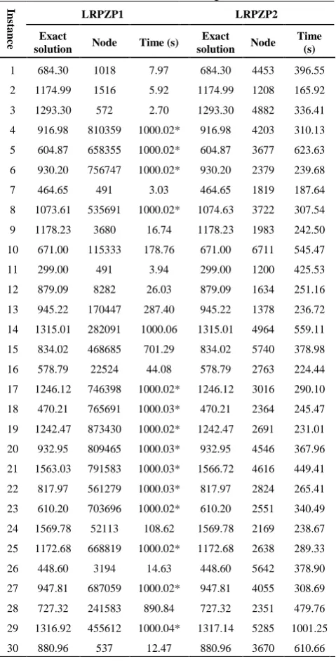
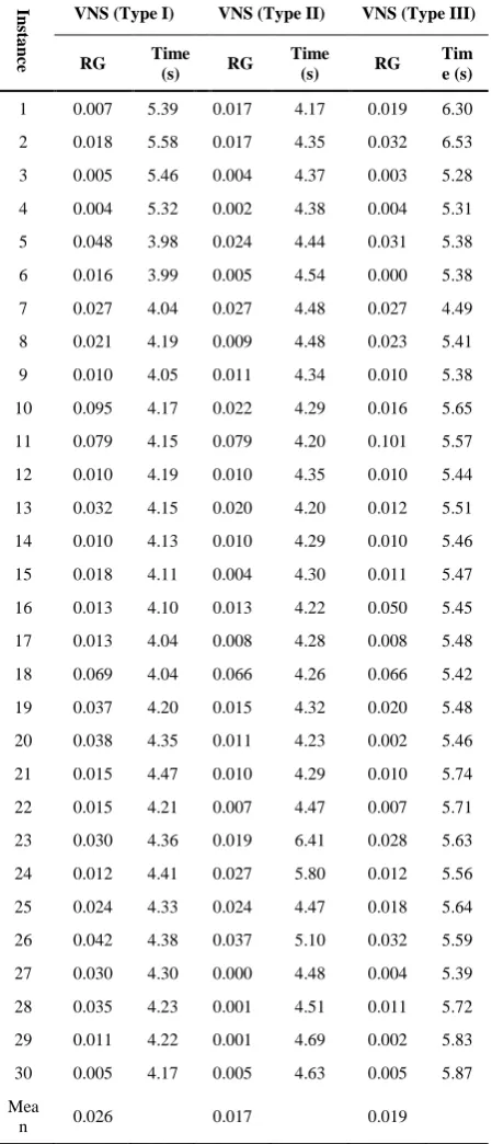
5. 1. Results In Table 2 and Table 3, we report the results to provide a basis for comparing the accuracy and efficiency of the two models and the proposed algorithm. The exact solutions of each model calculated by CPLEX are shown in columns "Exact solution". Number of used nodes in the branch and bound tree is available in column "Node". Columns "Time" represents the solution time of each approach. After running LRPZP1 in CPLEX software, CPLEX cannot find the exact solution for some instances. Moreover, CPLEX cannot find the exact solution in one hour (3600s). However, LRPZP2 finds the exact solution in all of the instances in a reasonable time. Objective function in all of the instances except the above mentioned instances, is the same. The column "RG" shows the relative gap between the exact solution and the solution of VNS algorithm. More analysis and some statistical tests are shown in the next subsection.
5. 2. Discussion and Statistical Analysis The statistic is widely employed in the field of research. In fact, it is almost impossible to come to an informed deduction in any part of the research without statistics. In this research, the results from statistical hypothesis tests (i.e., paired student's T-tests), show LRPZP2 uses less time for obtaining an exact solution versus LRPZP1 with a 0.05 significance level. The results of the hypothesis test are presented in Table 4. In addition, hypothesis test proves the used node for the branch and bound tree in LRPZP2 is less than LRPZP1. These results show the comparative superiority of LRPZP2 over LRPZP1 in performance. The proposed VNS algorithm shows a good performance in approximating the objective functions. The mean of RG for all instances in the VNS (type I), the VNS (type II) and the VNS (type III) are 0.02628, 0.01681 and 0.01935, respectively.
TABLE 1. Description of operators
Operator Definition
1-1 Move For two selected nodes, the first node is omitted from its current position and is placed after the second node.
1-Exchange For two selected nodes, they swap their positions.
2-Exchange
For two selected nodes, the first node and its successor exchange their positions with the second node and its successor.
2-Opt
For two selected nodes, the two arcs connecting them with their successors are omitted, the nodes are linked, their successors are linked, and finally the chain between the successor of the first node and the second node is reversed.
TABLE 2. Results of running two models
In
st
a
n
ce
LRPZP1 LRPZP2 Exact
solution Node Time (s)
Exact solution Node
Time (s)
1 684.30 1018 7.97 684.30 4453 396.55
2 1174.99 1516 5.92 1174.99 1208 165.92
3 1293.30 572 2.70 1293.30 4882 336.41
4 916.98 810359 1000.02* 916.98 4203 310.13
5 604.87 658355 1000.02* 604.87 3677 623.63
6 930.20 756747 1000.02* 930.20 2379 239.68
7 464.65 491 3.03 464.65 1819 187.64
8 1073.61 535691 1000.02* 1074.63 3722 307.54
9 1178.23 3680 16.74 1178.23 1983 242.50
10 671.00 115333 178.76 671.00 6711 545.47
11 299.00 491 3.94 299.00 1200 425.53
12 879.09 8282 26.03 879.09 1634 251.16
13 945.22 170447 287.40 945.22 1378 236.72
14 1315.01 282091 1000.06 1315.01 4964 559.11
15 834.02 468685 701.29 834.02 5740 378.98
16 578.79 22524 44.08 578.79 2763 224.44
17 1246.12 746398 1000.02* 1246.12 3016 290.10
18 470.21 765691 1000.03* 470.21 2364 245.47
19 1242.47 873430 1000.02* 1242.47 2691 231.01
20 932.95 809465 1000.03* 932.95 4546 367.96
21 1563.03 791583 1000.03* 1566.72 4616 449.41
22 817.97 561279 1000.03* 817.97 2824 265.41
23 610.20 703696 1000.02* 610.20 2551 340.49
24 1569.78 52113 108.62 1569.78 2169 238.67
25 1172.68 668819 1000.02* 1172.68 2638 289.33
26 448.60 3194 14.63 448.60 5642 378.90
27 947.81 687059 1000.02* 947.81 4055 308.69
28 727.32 241583 890.84 727.32 2351 479.76
29 1316.92 455612 1000.04* 1317.14 5285 1001.25
30 880.96 537 12.47 880.96 3670 610.66
* CPLEX cannot find exact solution for these instances and we run them for one hour (3600s)
TABLE 3. Results of running VNS
In
st
a
n
ce
VNS (Type I) VNS (Type II) VNS (Type III)
RG Time (s) RG
Time (s) RG
Tim e (s)
1 0.007 5.39 0.017 4.17 0.019 6.30
2 0.018 5.58 0.017 4.35 0.032 6.53
3 0.005 5.46 0.004 4.37 0.003 5.28
4 0.004 5.32 0.002 4.38 0.004 5.31
5 0.048 3.98 0.024 4.44 0.031 5.38
6 0.016 3.99 0.005 4.54 0.000 5.38
7 0.027 4.04 0.027 4.48 0.027 4.49
8 0.021 4.19 0.009 4.48 0.023 5.41
9 0.010 4.05 0.011 4.34 0.010 5.38
10 0.095 4.17 0.022 4.29 0.016 5.65
11 0.079 4.15 0.079 4.20 0.101 5.57
12 0.010 4.19 0.010 4.35 0.010 5.44
13 0.032 4.15 0.020 4.20 0.012 5.51
14 0.010 4.13 0.010 4.29 0.010 5.46
15 0.018 4.11 0.004 4.30 0.011 5.47
16 0.013 4.10 0.013 4.22 0.050 5.45
17 0.013 4.04 0.008 4.28 0.008 5.48
18 0.069 4.04 0.066 4.26 0.066 5.42
19 0.037 4.20 0.015 4.32 0.020 5.48
20 0.038 4.35 0.011 4.23 0.002 5.46
21 0.015 4.47 0.010 4.29 0.010 5.74
22 0.015 4.21 0.007 4.47 0.007 5.71
23 0.030 4.36 0.019 6.41 0.028 5.63
24 0.012 4.41 0.027 5.80 0.012 5.56
25 0.024 4.33 0.024 4.47 0.018 5.64
26 0.042 4.38 0.037 5.10 0.032 5.59
27 0.030 4.30 0.000 4.48 0.004 5.39
28 0.035 4.23 0.001 4.51 0.011 5.72
29 0.011 4.22 0.001 4.69 0.002 5.83
30 0.005 4.17 0.005 4.63 0.005 5.87
Mea
n 0.026 0.017 0.019
Moreover, the results confirmed when the solution time is the main factor for DM, the best alternatives are VNS (Type II) and VNS (Type I) between all proposed models and approaches. Another advantage of our algorithm is using less time compared to LRPZP1 and LRPZP2 and hypothesis tests accept this claim at the significance level 0.05.
TABLE 4. Results of hypothesis tests
Hypothesis test P-value
H0: Solution time of LRPZP2 is greater than or equal to
solution time of LRPZP1 0.019
H0: Used nodes for B&B in LRPZP2 is greater than or
equal to LRPZP1 0.000
H0: The solution time of the VNS (Type I) is less than or
equal to the solution time of LRPZP1 1.000
H0: The solution time of the VNS (Type I) is less than or
equal to the solution time of LRPZP2 1.000
H0: The solution time of the VNS (Type II) is less than
or equal to the solution time of LRPZP1 1.000
H0: The solution time of the VNS (Type II) is less than
or equal to the solution time of LRPZP2 1.000
H0: The solution time of the VNS (Type III) is less than
or equal to the solution time of LRPZP1 1.000
H0: The solution time of the VNS (Type III) is less than
or equal to the solution time of LRPZP2 1.000
H0: The solution time of the VNS (Type II) is equal to
the solution time of the VNS (Type I) 0.108
H0: The solution time of the VNS (Type II) is less than
or equal to the solution time of the VNS (Type III) 1.000
H0: The solution time of the VNS (Type I) is less than or
equal to the solution time of the VNS (Type III) 1.000
H0: The RG of the VNS (Type II) is less than or equal
the RG of the VNS (Type I) 0.998
H0: The RG of the VNS (Type II) is less than or equal
the RG of the VNS (Type III) 0.911
H0: The RG of the VNS (Type I) is less than or equal the
RG of the VNS (Type III) 0.031
6. CONCLUSION
algorithm over two models based on solution time. We suggest three types of combinations for the local search of the algorithm.
The second type gets the best performance between all of them. In this type, order of operators is indicated by generating random integer numbers between one and four.
If the generated number is set at one, 1-Exchange should be operated. In case of two, 1-1 Move is run after 1-Exchange. In the case of three, 2-Opt is also performed. Finally, in the case of four, 2-Exchange should be applied after the previous operators. The performance of this heuristic in terms of both accuracy and efficiency is considered to be quite promising, according to our computational results obtained on 30 randomly generated instances. As a future research direction, we intend to focus on LRPZP in a competitive situation. The firm can be considered as an entrant that wants to enter a big market in the presence of incumbents. It should make a decision about price, vehicle route and selecting depots. Another research direction is to examine our problem by taking into account the quality-dependent price of demands, since, another key factor for the customers is the level of feature and quality.
7. REFERENCES
1. Christian, R.C., "Physical distribution: Key to improved volume and profits", Journal of Marketing, Vol. 29, (1965), 65-70.
2. Aras, N., Aksen, D. and Tekin, M.T., "Selective multi-depot vehicle routing problem with pricing", Transportation Research Part C: Emerging Technologies, Vol. 19, No. 5, (2011), 866-884.
3. Lederer, P.J. and Thisse, J.-F., "Competitive location on networks under delivered pricing", Operations Research Letters, Vol. 9, No. 3, (1990), 147-153.
4. Phlips, L., "The economics of price discrimination, Cambridge University Press, (1983).
5. Hansen, P., Peeters, D. and Thisse, J.F., "Facility location under zone pricing", Journal of Regional Science, Vol. 37, No. 1, (1997), 1-22.
6. Lee, Y., Kim, S.-i., Lee, S. and Kang, K., "A location-routing problem in designing optical internet access with wdm systems",
Photonic Network Communications, Vol. 6, No. 2, (2003), 151-160.
7. Billionnet, A., Elloumi, S. and Djerbi, L.G., "Designing radio-mobile access networks based on synchronous digital hierarchy rings", Computers & operations research, Vol. 32, No. 2, (2005), 379-394.
8. Setak, M., Karimi, H. and Rastani, S., "Designing incomplete hub location-routing network in urban transportation problem",
International Journal of Engineering-Transactions C: Aspects, Vol. 26, No. 9, (2013), 997-1006.
9. Setak, M., Bolhassani, S.J. and Karimi, H., "A node-based mathematical model towards the location routing problem with intermediate replenishment facilities under capacity constraint",
International Journal of Engineering-Transactions C: Aspects, Vol. 27, No. 6, (2013), 911-920.
10. Tuzun, D. and Burke, L.I., "A two-phase tabu search approach to the location routing problem", European Journal of Operational Research, Vol. 116, No. 1, (1999), 87-99. 11. Beckmann, M.J. and Ingene, C.A., "The profit equivalence of
mill and uniform pricing policies", Regional Science and Urban Economics, Vol. 6, No. 3, (1976), 327-329.
12. Hansen, P., Thisse, J.-F. and Hanjoul, P., "Simple plant location under uniform delivered pricing", European Journal of Operational Research, Vol. 6, No. 2, (1981), 94-103.
13. Hurter, A.P. and Lederer, P.J., "Spatial duopoly with discriminatory pricing", Regional Science and Urban Economics, Vol. 15, No. 4, (1985), 541-553.
14. Kats, A., "Location-price equilibria in a spatial model of discriminatory pricing", Economics Letters, Vol. 25, No. 2, (1987), 105-109.
15. Hansen, P., Peeters, D. and Thisse, J.-F., "The profit-maximizing weber problem", Location Science, Vol. 3, No. 2, (1995), 67-85.
16. Dasci, A. and Laporte, G., "Location and pricing decisions of a multistore monopoly in a spatial market", Journal of Regional Science, Vol. 44, No. 3, (2004), 489-515.
17. Diakova, Z. and Kochetov, Y., "A double vns heuristic for the facility location and pricing problem", Electronic Notes in Discrete Mathematics, Vol. 39, (2012), 29-34.
18. Luer-Villagra, A. and Marianov, V., "A competitive hub location and pricing problem", European Journal of Operational Research, Vol. 231, No. 3, (2013), 734-744. 19. Hanjoul, P., Hansen, P., Peeters, D. and Thisse, J.-F.,
"Uncapacitated plant location under alternative spatial price policies", Management Science, Vol. 36, No. 1, (1990), 41-57. 20. Tofigh, A. and Mahmoudi, M., "Application of game theory in
dynamic competitive pricing with one price leader and n dependent followers", International Journal of Engineering-Transactions A: Basics, Vol. 25, No. 1, (2011), 35-44. 21. Miller, C.E., Tucker, A.W. and Zemlin, R.A., "Integer
programming formulation of traveling salesman problems",
Journal of the ACM (JACM), Vol. 7, No. 4, (1960), 326-329. 22. Wong, R.T., "Integer programming formulations of the traveling
salesman problem", in Proceedings of the IEEE international conference of circuits and computers, IEEE Press Piscataway, NJ., (1980), 149-152.
23. Mladenovic, N. and Hansen, P., "Variable neighborhood search", Computers & operations research, Vol. 24, No. 11, (1997), 1097-1100.
24. Melian, B. and Mladenovic, N., "Editorial", IMA Journal of Management Mathematics, Vol. 18, No. 2, (2007), 99-100. 25. Clarke, G.u. and Wright, J.W., "Scheduling of vehicles from a
Investigating Zone Pricing in a Location-Routing Problem Using a Variable
Neighborhood Search Algorithm
M. Setaka, M. Sadeghi-Dastakia, H. Karimi b
a Department of Industrial Engineering, K.N.Toosi University of Technology b Department of Industrial Engineering, University of Bojnord
P A P E R I N F O
Paper history:
Received 25 April 2015
Received in revised form 04 October 2015 Accepted 16 October 2015
Keywords: Pricing, Zone Pricing Location-Routing Problem Variable Neighborhood Search
ديكچ ه
رد یزاس هنیشیب فده اب ،هیحان ره رد وپد ناکم و هیلقن هلیسو ریسم ،تمیق هنیهب نییعت لابند هب هک هدش هتفرگ رظن رد یتکرش ،هلاقم نیا
یم دوس دشاب ؛ تمیق عوضوم ،هلاقم نیا نیاربانب هقطنم یراذگ
ناکم لئاسم تایبدا دراو ار یا یبای
-ریسم تمیق .تسا هدرک یبای یراذگ
هقطنم تسایس نیرتمهم زا یکی یا تمیق یاه
تکرش زا یرایسب طسوت هک تسا یراذگ یم رارق هدافتسا دروم اه
یداهنشیپ هلاسم .دریگ
لثم یتلاوصحم عیزوت رد م
نرب لدم .تسا هدش یدنبلومرف نایرج و هرگ رب ینتبم لدم ود طسوت هلاسم .دراد ناوارف دربراک هوی هما
یزیر
هعطق شور کی طسوت ،هدمآ تسدب یطخریغ حیحص ددع هعظق
هب .تسا هتفرگ رارق هسیاقم دروم اهنآ درکلمع و دش هدز بیرقت یطخ
یراگزاس روظنم اب
بیکرت هس .دیدرگ ارجا هلاسم یدادعت یارب و تفای هعسوت ریغتم یگیاسمه یوجتسج متیروگلا کی ،یعقاو یایند
رعم یلحم یوجتسج فلتخم تابساحم زا لصاح جیاتن .تفرگ رارق هسیاقم دروم یداهنشیپ لدم ود اب زین و مه اب اهنآ درکلمع و دش یف
لدم یاج هب گرزب لئاسم لح رد یداهنشیپ متیروگلا ییاراک یم دییات ار یداهنشیپ یاه
دیامن
.
یم ناشن جیاتن هولاع هب لدم هک دنهد
مک یتابساحم نامز نایرج رب ینتبم یم هدافتسا هرگ رب ینتبم لدم تبسن هب ار یرت
.دیامن