Fault Type Estimation in Power Systems
J. Beiza*, S. H. Hosseinian* and B. Vahidi*
Abstract: This paper presents a novel approach for fault type estimation in power systems. The Fault type estimation is the first step to estimate instantaneous voltage, voltage sag magnitude and duration in a three-phase system at fault duration. The approach is based on time-domain state estimation where redundant measurements are available. The current based model allows a linear mapping between the measured variable and the states to be estimated. This paper shows a possible for fault instance detection, fault location identification and fault type estimation utilizing residual analysis and topology error processing. The idea is that the fault status does not change measurement matrix dimensions but changes some elements of the measurement matrix. The paper addresses how to rebuilt measurement matrix for each type of faults. The proposed algorithm is shown that the method has high effectiveness and high performance for forecasting fault type and for estimating instantaneous bus voltage. The performance of the novel approach is tested on IEEE 14-bus test system and the results are shown.
Keywords: Fault type, Power system quality, State estimation, Residual analysis.
1 Introduction1
Fault is one of the reasons for voltage sag in power systems. Voltage sag is the most concern to electric utilities and consumers. According to the IEEE standard 1346 voltage sag is a decrease in root-mean-square (rms) voltage at the power frequency for durations of 0.5 cycles to 1 min. Typical voltage sag values are 0.1 to 0.9 pu [1]. In most of studies related to voltage sag analysis the power system is considered as a balanced system. Therefore, this assumption can allow the use of single-phase modeling for entire network. But most short circuits cause unbalanced condition in power systems.
Three-phase (symmetrical) faults lead to severe sags at a large number of buses over the wide geographical region (depending on the network topology). These faults fortunately, are very rare in the power system. Single phase-to-ground fault and other asymmetrical faults (phase-to-phase and double-phase-to-ground faults) typically cause sags with higher magnitudes (voltage sag magnitude being defined as the magnitude of the remaining voltage at the bus), however, they are much more common in power systems [2]. Probability of single ground fault is 80%, double
Iranian Journal of Electrical & Electronic Engineering, 2009. Paper first received 2 May 2009 and in revised form 7 Jun. 2009. * The Authors are with the Department of Electrical Engineering, Amirkabir University, Tehran, Iran.
E-mails: [email protected], [email protected] and
ground fault is 17%, phase-to-phase fault is 2%, and three-phase fault is 1% [3]. As a result, it is necessary to assess voltage sag in a three-phase system.
There are many researches about voltage sag stochastic assessment. Most of them are based on critical distance and fault positions where combines stochastic data concerning the fault likelihood with deterministic data regarding the residual voltages during the occurrence of faults. The probabilistic nature of stochastic methods makes them suitable for long term estimations, but in a specific year, the predicted number of voltage sags can differ substantially from the measurement. In addition, in some cases, historic data are not available when analyzing a part of the system recently introduced or modified [4]. Also, monitoring of voltage sag indices are needed to calibrate stochastic methods. In addition, dynamic performance of the power system is neglected in most of the stochastic assessments which is most effects on voltage sag indices. As a result, there is a gap to overcome the aforementioned shortcoming of stochastic procedures. In order to fill this gap, it is necessary to monitor Instantaneous voltage in time domain which is fulfilled on state estimation (SE).
In order to identify the current operating state of the system, state estimators facilitate accurate and efficient monitoring of the power system. State estimation is a fundamental tool for control and monitoring of electrical power systems. State estimation is required to produce a best estimation of state variables and to
detect, identify and surpass gross measurement errors and to product an estimate of non-metered or lost data points. Also, State estimation is one of the essential functions in energy management systems (EMS). Nowadays, in supervisory control and data acquisition (SCADA) control centers (C.C), EMS servers execute real time state estimation. Weighted Least Square (WLS) state estimation algorithm is used to solve the normal equation widely [5]. It is necessary to say that traditional SCADA monitoring system is not suitable for this application because the scanning of signal is very low.
In the voltage sag state estimation procedure, it is necessary to estimate instantaneous voltage at any time. When a fault is occurred, there is one topology error. At the first step, it is important to estimate type of fault. The estimation is used to forecast how to rebuild measurement matrix for next step of instantaneous voltage estimation after fault instance. Accordingly, the main application of the proposed method is to consider new algorithm for estimating type of fault in a three-phase system and for rebuilding measurement equations for time - domain voltage sag state estimation.
There are several researches for fault classification and fault location algorithm which are based on synchronized sampling of the voltage and current data from one end or multi ends of transmission line [7, 8].
Wide area monitoring (WAM) and clock synchronization were not feasible up to a few years ago. Communication technologies simply were not available to handle the demands imposed by the complexity of WAM requirements. But, nowadays, communication standards have been developed to be able to address many of these demands [6]. According to the above issues, there is not any concern about WAM, clock synchronization and real time implementation challenges. It is necessary to say that the goal of the power system voltage sag monitoring is not to determine preventive actions in order to maintain the system in the normal secure state. Therefore, real time implementation is unnecessary for this application. But clock synchronization signal must be available for synchronization. At this state, GPS (Globally Positioning System) time signal plays the best role for removing the challenges.
The remainder of the paper is organized as follows. In section 2, fundamental concepts of state estimation are described. Section 3 discusses the time domain state estimation. In section 4, fault detection and identification is described, which includes time domain measurement matrix and residual analysis. New algorithm for fault type estimation is illustrated in section 5. Numerical results are shown in section 6. Finally, conclusions are noted in section 7.
2 State Estimation
State Estimation (SE) was introduced by Gauss and Legendre in 18th century. The basic idea was to "fine-tune" state variables by minimizing the sum of the residual squares. This is the well-known least squares (LS) method. The other method is the Weighted Least Square (WLS). The method is used to minimize the weighted sum of the residual squares. WLS calculates the best estimation of states [9, 10]. In fact, the measurement errors are assumed to have a known probability density function. Most of time, Gaussian (normal) distribution probability density functions with zero mean value and known variance is used. Another objective of SE is detection, identification and suppression of gross measurement errors [11]. In this paper, the aforementioned subject is developed to detect fault location in order to voltage sag estimation.
Consider the set of measurements given by vector z [12]:
1 1 1 2 n 1
2 2 1 2 n 2
m m 1 2 n m
z h (x , x ,..., x ) e
z h (x , x ,..., x ) e
. . .
z h(x) e
. . .
. . .
z h (x , x ,..., x ) e
⎡ ⎤ ⎡ ⎤ ⎡ ⎤
⎢ ⎥ ⎢ ⎥ ⎢ ⎥
⎢ ⎥ ⎢ ⎥ ⎢ ⎥
⎢ ⎥ ⎢ ⎥ ⎢ ⎥
=⎢ ⎥ ⎢= ⎥ ⎢+ ⎥= +
⎢ ⎥ ⎢ ⎥ ⎢ ⎥
⎢ ⎥ ⎢ ⎥ ⎢ ⎥
⎢ ⎥ ⎢ ⎥ ⎢ ⎥
⎢ ⎥ ⎢ ⎥ ⎢ ⎥
⎣ ⎦ ⎣ ⎦ ⎣ ⎦
(1)
where, h (x)i is the nonlinear function relating i-th measurement to the states, xi is the state, m is the number of measurements and n is the number of states. Also,
x
is the system state vector and e is the measurement error vector. Equation (1) is named as measurement equation.Regarding the statistical properties of the measurement errors, the following assumptions are made:
i
E(e )=0, i=1, 2,..., m (2)
i j
E(e .e )=0, i=1, 2,..., m (3)
Equations (2) and (3) express that the mean values of measurements errors vectors are zero, and also the measurement errors are independent. Hence,
T 2 2 2
1 2 m
Cov(e)=E(e.e )= =R diag(σ σ, ,...,σ ) (4)
where,σi is the standard deviation for measurement i which is computed to reflect the expected accuracy of the corresponding meter used.
Now, objective function is defined as follows:
m
2
i i ii
i 1
T 1
J(x) (z h (x)) / R
[z h(x)] R [z h(x)]
= −
= −
= − −
∑
(5)
Finally, the weighted least squares state estimation leads to an iterative solution of the following equation namely Normal Equation (NE) [12]:
k 1 k T k
k) x H (x )R z
x (
G Δ = −Δ (6)
where, H is measurement Jacobian matrix of h(x), G is
gain matrix and is equal to H R HT −1 and k denotes the iteration index.
The residual index is as follows:
r= Δ = −z z H(x) (7)
In the conventional power system telemetry stations, both active power and reactive power are analogue measurements. If these parameters are chosen as set of measurements and bus voltages are chosen as states then measurement equation is nonlinear. Decoupled weighted least squares state estimation is introduced to have linear measurement equation [12]. Also, when line currents and some bus voltages are chosen as state variables, measurement equation becomes linear [13].
In linear measurement equation:
z=Hx+e (8)
In this case the objective function is:
T 1
J(x)= −[z Hx] R [z− −Hx] (9)
In order to have a unique solution, linear equation must be completely determined or over determined. At these conditions, the system state vector is estimated as follows [5], [9]:
z R H G
xestimated = −1 T −1 (10)
Network observability analysis must be checked prior to SE. This analysis will be determined if a unique estimate can be found for the system states [12, 14].
In this paper, according to [14] the network observability analysis is done to determine observability of the network.
3 Time Domain State Estimation
Time domain state estimation requires time domain modeling of power system components and some assumptions in power system. These assumptions allow the use of single phase circuit for modeling power system. If measurement sets are placed on the lines, main component for state estimation in power system is line or branch modeling. Therefore, the following issues are concentrated to develop line modeling for time domain state estimation.
The pi line model is used to show equivalent circuit for a line in power system. The standard differential voltage-current relationships for resistor, inductor and capacitor elements are given at [15]:
RL RL RL
RL
1 1
i (t) v (t) v (t t)
2L 2L
(1 )R (1 )R
t t
2L
(1 )R
t i (t t) 2L
(1 )R t
+α −α
= + −Δ
+ +α + +α
Δ Δ
− −α Δ
+ −Δ
+ +α Δ
(11)
C C C
C
2C 2C
i (t) v (t) v (t t) t(1 ) t(1 )
1
i (t t) 1
= − − Δ
Δ + α Δ + α
− α
− − Δ
+ α
(12)
where α is the compensating constant factor,
RL RL
v (t),i (t) are the voltage and current of the series
branch, respectively and v (t), i (t)C C are the voltage and current across shunt branch, respectively. Also, R,L, and C are the values of resistance, inductance and capacitance of the line, respectively.
Let Xt represents the vector of all bus voltages at time t. Then the measurement equation can be written as:
t m h t
Z =i (t) i (t)− =HX (13)
where, Xt,im(t) are the vector of all bus voltages and measurement current at t instance, respectively. Also, H and i (t)h are measurement matrix in time domain and history term of components at t instance, respectively. The mth row of corresponding to the mth branch between buses k and j is obtained as follows:
kj
kj
kj
2C 1
H(m, i)
2L
t(1 )
(1 )R
t
+ α
= +
Δ + α
+ + α Δ
(14)
kj
kj
1 H(m, j)
2L
(1 )R
t
+ α = −
+ + α Δ
(15)
where α is a constant referred as the compensating factor, which is zero for the trapezoidal approach.
Assuming there are Nm measurements and Ns
states (bus voltages), then im(t) is a vector of
measurements, H is the Nm×Ns measurement matrix,
Xt is a Nsvector of bus voltages, and i (t)h is an
Nmvector of history terms. Instantaneous bus voltages
are then calculated using (10).
4 Fault Detection and Identification Approach
SE has typically several functions. One of these functions is topology error processing. The topology error processing can be classified in two categories:
branch status error and configuration error. When a fault is occurred, there is one topology error. It is categorized as branch status error. In the fault status, the measurement matrix dimensions are not changed but some elements of the measurement matrix are changed. This subject is described in the following.
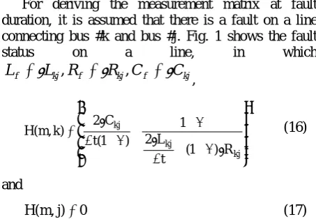
For deriving the measurement matrix at fault duration, it is assumed that there is a fault on a line connecting bus #k and bus #j. Fig. 1 shows the fault status on a line, in which
kj f kj f kj
f L R R C C
L =
γ
, =γ
, =γ
,
kj
kj
kj
2 C 1
H(m, k)
2 L t(1 )
(1 ) R t
⎛ ⎞
⎜ γ + α ⎟
⎜ ⎟
= +
γ Δ + α
⎜ + + α γ ⎟
⎜ Δ ⎟
⎝ ⎠
(16)
and
H(m, j)=0 (17)
where γ is fault distance and R , L , C
kj kj kj are values of
resistance, inductance and capacitance of the line. The proposed approach combines two test methods for fault detection and identification. The main idea is that when there is a fault, there is a single error on network topology at fault duration. The selected methods are the largest normalized residual test and residual analysis. They are based on residual value and residual mean value, respectively.
The largest normalized residual test can be used to devise a test for identifying and detecting a single error [12].
The test has the following steps: 1. Solve WLS to obtain residual vector. 2. Compute the normalized residuals as follows:
i N i
ii r
r = , i=1, 2,..., m
Ω (18)
where, m is the number of measurements and Ω is the
residual covariance matrix. Ifr N
k > δ, then there is a fault, δ is chosen as a threshold for fault detection.
Fig. 1. The fault status on a line
It is necessary to say that fault location must be determined to solve SE. In other words, measurement matrix at the steady state is different from measurement matrix at fault duration. In this case, a method is required to detect and identify on which line or branch the fault occurs. The proposed approach uses the residual analysis concept to determine fault location and to rebuild measurement matrix.
Basic point in fault status is the fact that measurement matrix dimensions are not changed. Therefore, the relation between measurement matrixes in two statues is described as [1, 16]:
fault steady
H =H +E (19)
where, E is the error measurement matrix. In fault duration SE equation is defined as:
fault steady
z=H x+ =e H x+Ex+e (20)
Before fault detection and identification, residual vector at fault duration is given as:
steadyˆ
r= −z H x (21)
Mean and covariance values for residual are expressed as:
E(r)= −(I K)Ex (22)
Cov(r)= −(I K)R (23)
where K is hat matrix as follows
1 T 1
steady steady
K=H G H− R− (24)
The following equation relates relationship between residuals and vector line error [17].
r=Tf (25)
where f is vector line error and T is given by:
T= −(I K)M (26)
where M is measurement - to - line incident matrix. According to the co linearity test which is described in [17] the dot product between T and r is as follows:
T j j
j T r cos
T r
θ = (27)
where T , rj are the largest singular value of
T ,rj ,respectively.
Line j has a short circuit fault if cos jθ is approximately equal to one. For other lines they are less than one. In this case, the two described methods with
power network topology at fault duration can be used to detect and identify fault as fault indices.
5 Fault Type Estimation Algorithm
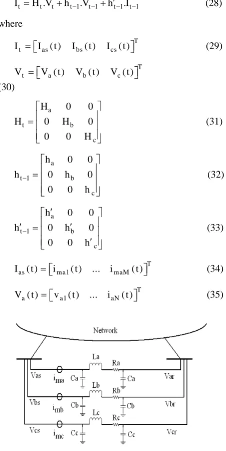
Time domain state estimation requires time domain modeling. At fault, power system network operates under unbalance condition for three-phase system. Therefore, it is necessary to develop measurement equation in the structure of three-phase system. In addition, the method can be used to estimate state variables under unbalance condition at steady state. Fig. 2 shows typical three-phase line of the network with current measurement connecting bus s and bus r. Measurement equation in a three-phase system at time domain is as follows:
t t t t 1 t 1 t 1 t 1
I =H .V +h−.V− +h′−.I− (28)
where
T
t as bs cs
I = ⎡⎣I (t ) I ( t ) I ( t )⎤⎦ (29)
T
t a b c
V = ⎡⎣V ( t ) V ( t ) V ( t )⎤⎦
(30)
a
t b
c
H 0 0
H 0 H 0
0 0 H
⎡ ⎤
⎢ ⎥
= ⎢ ⎥
⎢ ⎥
⎣ ⎦
(31)
a
t 1 b
c
h 0 0
h 0 h 0
0 0 h
−
⎡ ⎤
⎢ ⎥
= ⎢ ⎥
⎢ ⎥
⎣ ⎦
(32)
a
t 1 b
c
h 0 0
h 0 h 0
0 0 h
−
′
⎡ ⎤
⎢ ⎥
′ = ⎢ ′ ⎥
⎢ ′ ⎥
⎣ ⎦
(33)
T
as ma1 maM
I ( t )= ⎡⎣i (t ) ... i ( t )⎤⎦ (34)
T
a a1 aN
V (t )= ⎡⎣v ( t ) ... i ( t )⎤⎦ (35)
Fig. 2. Typical three-phase line of the network with measurement set
in which N is number of buses and M is number of measurements.
When a fault is occurred, fault zone is determined using fault detection and identification method which is described is section 4. Type of fault forecasting and measurement equation structure rebuilding are described in the following subsections.
5.1 Single-Phase-to-Ground Fault (SLG)
Assume there is a single-line-to-ground fault in phase A of line m. At this condition, the largest element of normalized residual vector can be compared against a statistical threshold to decide about the existence of a fault. This threshold can be chosen based on the desired level of detection sensitivity. The normalized residual vector related to phase A measurement will be increased at the fault. Also, theta cosine index vector related to phase A, for the line m, will be approximately equal to one. State estimation procedure detects and identifies line-to-ground fault type. The duration of estimation is one time step after fault instance. After this conduction, measurement matrix is rebuilt as follows:
fa rsa fa rsa fa rsa
C = γC , L = γL , R = γR (36)
fa a
fa
fa
2C 1
H (m, s)
2L
t(1 )
(1 )R
t
⎡ ⎤
⎢ + α ⎥
=⎢ + ⎥
Δ + α
⎢ + + α ⎥
⎢ Δ ⎥
⎣ ⎦
(37)
a
H (m, r)=0 (38)
fa a
fa
fa
2C 1
h (m, s)
2L
t(1 )
(1 )R
t
⎡ ⎤
⎢ − α ⎥
=⎢ + ⎥
Δ + α
⎢ + + α ⎥
⎢ Δ ⎥
⎣ ⎦
(39)
a
h (m, r)=0 (40)
where measurement m is located on line k. Measurement matrixes for other two phases do not change and assuming fault resistance is zero.
5.2 Two-Phase-to-Ground Fault (LLG)
When two-phase-to-ground fault is occurred, for example between phase A and phase B, fault indices for two phases are increased. But there is not any difference between this condition and phase-to-phase fault condition. The increscent for two condition are the same and unable to detect. The proposed solution is that state estimation is done based on two-phase-to-ground fault condition after that fault indices are calculated again. In that case, measurement matrix can be calculated as:
fq rsq fq rsq fq rsq
C = γC , L = γL , R = γR (41)
fq q
fq
fq
2C 1
H (m, s)
2L
t(1 )
(1 )R
t
⎡ ⎤
⎢ + α ⎥
⎢ ⎥
= +
Δ + α
⎢ + + α ⎥
⎢ Δ ⎥
⎣ ⎦
(42)
q
H (m, r)=0 (43)
fq q
fq
fq
2C 1
h (m, s)
2L
t(1 )
(1 )R
t
⎡ ⎤
⎢ − α ⎥
⎢ ⎥
= +
Δ + α
⎢ + + α ⎥
⎢ Δ ⎥
⎣ ⎦
(44)
q
h (m, r)=0 (45)
where q=a, b. In fact, equations are valid for phase A and phase B. If fault indices can be returned to steady state zones then the assumption is true. Otherwise, there is phase-to-phase fault. The mentioned determination is done at one step time duration.
5.3 Phase-to-Phase Fault (LL)
In steady state condition, current measurement at sending end for phase A depends on what happened at sending end voltage and receiving end voltage in phase A at same time and at one step time earlier. When LLG fault is occurred, the dependency at receiving end voltage in phase A and phase B is neglected. This subject is implemented using equations (46), (50).
In LL fault, current measurement at sending end for phase A, approximately, depends on what happened at sending end voltage in phase A and B at the same time and at one step time earlier. There is same condition for the current measurement at sending end for phase B.
Therefore, measurement matrixes are illustrated as follows:
a
H (m, r)=0 (46)
a
h (m, r)=0 (47)
ba a
H (m, s)= −H (m, s) (48)
ba a
h (m, s)= −h (m, s) (49)
b
H (m, r)=0 (50)
b
h (m, r)=0 (51)
ab b
H (m, s)= −H (m, s) (52)
ab b
h (m, s)= −h (m, s) (53)
where
a ba
t ab b
c
H H 0
H H H 0
0 0 H
⎡ ⎤
⎢ ⎥
= ⎢ ⎥
⎢ ⎥
⎣ ⎦
(54)
a ba
t 1 ab b
c
h h 0
h h h 0
0 0 h
−
⎡ ⎤
⎢ ⎥
= ⎢ ⎥
⎢ ⎥
⎣ ⎦
(55)
5.4 Three-Phase Symmetric Fault (LLL)
Three-phase fault and three-phase-to-ground fault cause to increase all the fault indices of the three phases. Therefore, measurement equation is constructed as the following:
fq rsq fq rsq fq rsq
C = γC , L = γL , R = γR (56)
fq q
fq
fq
2C 1
H (m, s)
2L
t(1 )
(1 )R
t
⎡ ⎤
⎢ + α ⎥
⎢ ⎥
= +
Δ + α
⎢ + + α ⎥
⎢ Δ ⎥
⎣ ⎦
(57)
q
H (m, r)=0 (58)
fq q
fq
fq
2C 1
h (m, s)
2L
t(1 )
(1 )R
t
⎡ ⎤
⎢ − α ⎥
⎢ ⎥
= +
Δ + α
⎢ + + α ⎥
⎢ Δ ⎥
⎣ ⎦
(59)
q
h (m, r)=0 (60)
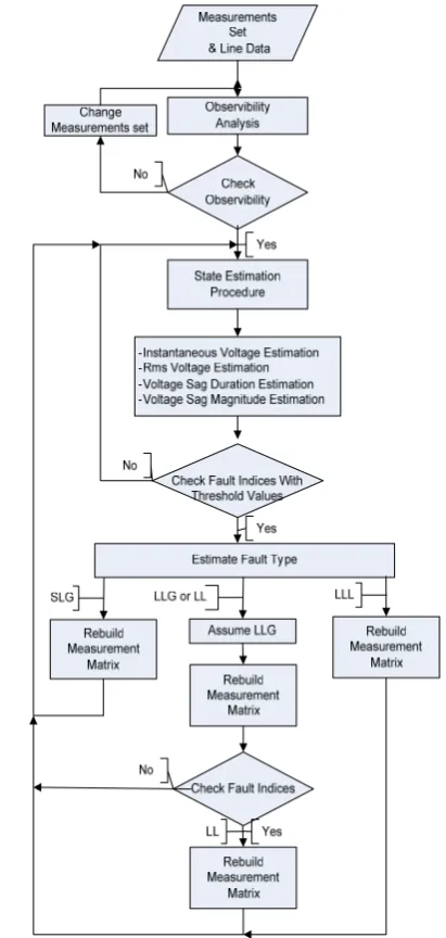
where q=a, b, c. In fact, equations are valid for phase A, phase B, and phase C. The algorithm for voltage sag estimation is summarized in Fig. 3.
6 Numerical Analysis
Since field data are not available, case studies based on simulated data are presented for demonstrating the effectiveness of the new algorithm. IEEE 14-bus test system is utilized to estimate state variable. The system with 15 lines, 3 transformers and 2 generators is used to simulate at the time domain [18]. The set of measurements are based on the method for observability analysis according to [14]. The method is used to guarantee fully observable network. The measurements placement description is illustrated in the appendix. The test system with measurement set is shown in Fig. 4.The system has 17 current measurements on lines and one voltage measurement on bus 1. The number of the measurements is relatively high compared to the number of the voltages to be estimated. It causes to guarantee the linear equation is over determined.
The power system is simulated in three-phase structure and in time domain. The Gaussian noise with zero mean and σ =0.1% is applied to all measured quantities. The simulation is done with 0.1 ms time step for 160 ms simulation time. Different fault types occur in the middle of line 4 at time 40 ms. Fault duration is assumed to be 4 cycles, assuming zero fault resistance.
Fig. 3. The novel algorithm in order to voltage sag estimation in a three-phase system
Fig. 4. IEEE 14-bus test system with measurement set
0 5 10 15 20 25 30 35 40 45 50 55 60
0 0.02 0.04 0.06 0.08 0.1 0.12 0.14
Measurement NO.
N
o
rm
al
iz
ed R
e
s
id
ual
I
n
d
e
x
(p.
u.
)
No Fault
Fig. 5. Normalized Residual Index for measurement set in three-phase at no fault
0 5 10 15 20 25 30 35 40 45 50 55 60
0 5 10 15 20 25 30
Measurement NO.
N
o
rm
a
liz
ed R
e
s
idual
I
n
d
e
x
(p.
u.
)
Three-Phase Fault
Phase A
Phase B Phase C
Fig. 6. Normalized Residual Index for measurement set at three-phase fault
Fig. 5 shows normalized residual values for all measurements in three-phase system at steady state condition. The measurements 1 to 18 are related to phase A, the measurements 19 to 36 are related to phase B and the measurements 37 to 54 are related to phase C. All of the values are under threshold condition so that there is not any fault. After LLL fault, these values are increased from threshold value. The aforementioned subject is depicted in Fig. 6. The figure shows that measurements number 17, 35 and 53 have quantity larger than other values. The measurements number 17, 35 and 53 are related to current measurement of phase A, B and C of line 4, respectively.
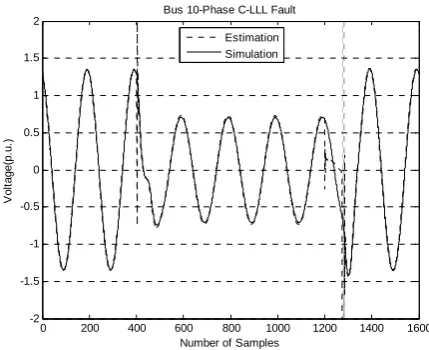
When fault is detected and identified, measurement equation must be rebuilt during the fault condition. This case requires fault type determination. The determination is based on fault index. It is clear that there is a LLL fault in Fig. 6. Therefore, measurement
matrix is rebuilt according to section 5. Instantaneous voltages (estimated and simulated) for bus 10 at both conditions (fault and steady state) are shown in Figs. 7, 8, and 9. These figures are for phase A, phase B and phase C, respectively.
For LLG fault analysis, a LLG fault was occurred in the middle of line 4 at time 40 ms. Fault duration is assumed to be 4 cycles. The comparisons between the instantaneous estimated voltages and the simulated voltages are illustrated in Figs. 10, 11, and 12. These figures are for bus 10 and for phase A, B and C, respectively. These figures demonstrate that instantaneous voltage estimation provided a good estimate of the system states and was capable of correctly detecting fault instance, identifying fault location, estimating fault type and rebuilding the measurement matrix.
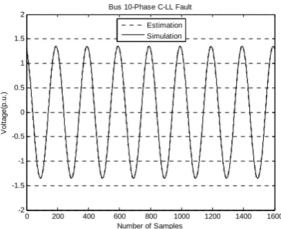
LL fault is considered in subsection 6.3. Figs. 13, 14 and 15 are for bus 10-phase A, bus 10-phase B and bus 10-phase C, respectively. Phase A and phase B are considered as faulted phases.
The estimated and simulated results are shown for SLG fault in Fig. 16 as dotted and solid lines, respectively. The figure includes phase A waveform, Phase B waveform and Phase C waveform. Phase A has fault status.
All plotted figures show that estimated voltages are coincided on the simulated voltages. In other word, both estimated and simulated results are indistinguishable due to similarity. Therefore, this lead to less error in estimated values so that these figures confirm the validation of the proposed algorithm.
7 Conclusion
In this paper, an efficient algorithm is applied to estimate fault type for instantaneous voltage estimation with more accurate estimation. Main application of the algorithm is considered for voltage sag estimation. It is clearly shown that different fault types can be detected and identified using the proposed fault indices. Threshold value for detecting fault depends on network parameters. In addition, it is shown that the largest normalized residual analysis and residual analysis can be used to estimate fault instance and to estimate fault location. Also, the results of estimated and simulated voltages emphasize the validation of the novel algorithm. With the proposed method, not only voltage sag magnitude but also voltage sag duration can be calculated. Generally, the proposed novel algorithm is suitable for other aspects of power quality monitoring as well as voltage sag.
6.1 Figures of Three-Phase Symmetric Fault (LLL)
0 200 400 600 800 1000 1200 1400 1600
-2 -1.5 -1 -0.5 0 0.5 1 1.5 2
V
o
lt
age(
p
.u.
)
Number of Samples Bus 10-Phase A-LLL Fault
Estimation Simulation
Fig. 7. Instantaneous voltage for phase A-bus #10 at LLL Fault (estimation and simulation)
0 200 400 600 800 1000 1200 1400 1600
-2 -1.5 -1 -0.5 0 0.5 1 1.5 2
V
o
lt
ag
e(
p.
u.
)
Number of Samples Bus 10-Phase B-LLL Fault
Estimation Simulation
Fig. 8. Instantaneous voltage for phase B-bus #10 at LLL Fault(estimation and simulation)
0 200 400 600 800 1000 1200 1400 1600
-2 -1.5 -1 -0.5 0 0.5 1 1.5 2
V
o
lt
ag
e(
p.
u.
)
Number of Samples Bus 10-Phase C-LLL Fault
Estimation Simulation
Fig. 9. Instantaneous voltage for phase C-bus #10 at LLL Fault(estimation and simulation)
6.2 Figures of Two-Phase-to-Ground Fault (LLG)
0 200 400 600 800 1000 1200 1400 1600
-2 -1.5 -1 -0.5 0 0.5 1 1.5 2
V
o
lt
a
ge(p.
u.
)
Number of Samples Bus 10-Phase A-LLG Fault
Estimation Simulation
Fig. 10. Instantaneous voltage for phase A-bus #10 at LLG Fault(estimation and simulation)
0 200 400 600 800 1000 1200 1400 1600
-2 -1.5 -1 -0.5 0 0.5 1 1.5 2
V
o
lt
a
ge(
p.
u.
)
Number of Samples Bus 10-Phase B-LLG Fault
Estimation Simulation
Fig. 11. Instantaneous voltage for phase B-bus #10 at LLG Fault (estimation and simulation)
0 200 400 600 800 1000 1200 1400 1600
-2 -1.5 -1 -0.5 0 0.5 1 1.5 2
V
o
lt
ag
e(
p.
u
.)
Number of Samples Bus 10-Phase C-LLG Fault
Estimation Simulation
Fig. 12. Instantaneous voltage for phase C-bus #10 at LLG Fault (estimation and simulation)
6.3 Figures of Phase-to-Phase Fault (LL)
0 200 400 600 800 1000 1200 1400 1600
-2 -1.5 -1 -0.5 0 0.5 1 1.5 2
V
o
lt
ag
e(
p
.u
.)
Number of Samples Bus 10-Phase A-LL Fault
Estimation Simulation
Fig. 13. Instantaneous voltage for phase A-bus #10 at LL Fault (estimation and simulation)
0 200 400 600 800 1000 1200 1400 1600
-2 -1.5 -1 -0.5 0 0.5 1 1.5 2
V
o
lt
ag
e(
p.
u.
)
Number of Samples Bus 10-Phase B-LL Fault
Estimation Simulation
Fig. 14. Instantaneous voltage for phase B-bus #10 at LL Fault (estimation and simulation)
0 200 400 600 800 1000 1200 1400 1600
-2 -1.5 -1 -0.5 0 0.5 1 1.5 2
Vo
lt
a
g
e
(p
.u
.)
Number of Samples Bus 10-Phase C-LL Fault
Estimation Simulation
Fig. 15. Instantaneous voltage for phase C-bus #10 at LL Fault (estimation and simulation)
6.4 Figure of Single-Phase-to-Ground Fault (SLG)
0 200 400 600 800 1000 1200 1400 1600
-2 -1.5 -1 -0.5 0 0.5 1 1.5 2 2.5 3
V
o
lt
a
ge(
p.
u.
)
Number of Samples Bus 10-Phase A,B,C-SLG Fault
Phase A PhaseB
Phase C
Fig. 16. Instantaneous voltage for phase A, B, C-bus #10 at SLG Fault (estimation and simulation)
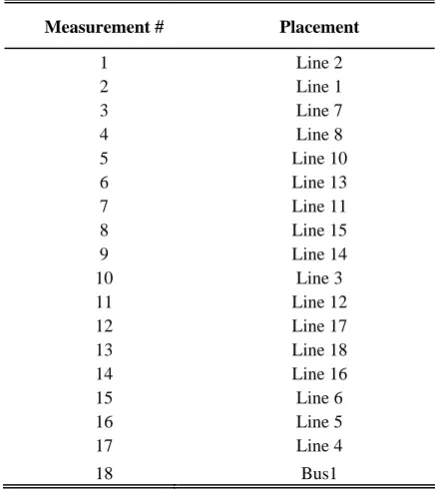
Table 1. Measurements Placement
Measurement # Placement
1 Line 2
2 Line 1
3 Line 7
4 Line 8
5 Line 10
6 Line 13
7 Line 11
8 Line 15
9 Line 14
10 Line 3
11 Line 12
12 Line 17
13 Line 18
14 Line 16
15 Line 6
16 Line 5
17 Line 4
18 Bus1
Appendix
The measurement placement for IEEE 14-bus is illustrated in Table 1.
References
[1] IEEE Recommended Practice for Evaluating Electric Power System Compatibility with Electronic Process Equipment, IEEE Standard 1346, 1998.
[2] Milanovic J. V., Aung M. T., and Gupta C. P., “The Influence of Fault Distribution on Stochastic Prediction of Voltage Sags”, IEEE
Transaction on power Delivery, Vol. 20, No. 1, pp. 278 – 285, January 2005.
[3] Martinez J., Martin-Arnedo J., “Voltage Sags Analysis Using an Electromagnetic Transient Program”.,IEEE Power Engineering Society Winter Meeting, Vol. 2, pp. 1135-1140, 2002. [4] Espinosa-Juarez E.and Hernandez A., “A Method
for Voltage Sag State Estimation in Power Systems”, IEEE Transaction on power delivery, Vol. 22, No. 4, pp. 2517-2526, Oct. 2007.
[5] Mazadi M., Hosseinian S. H., Rosehart W.and Westwick D. T., “Instantaneous Voltage Estimation for Assessment and Monitoring of Flicker Indices in Power Systems”, IEEE Transaction on power delivery, Vol. 22, No. 3, pp. 1841-1846, July 2007.
[6] Guidelines for Implementing Substation Automation Using IEC 61850, the International Power System Information Modeling Standard. Final Report, EPRI, Palo Alto, CA: 2004.1008688.
[7] Ha H., Zhang B. and Lv Z., “A Novel Principle of Single-Ended Fault Location Technique for EHV Transmission Lines”, IEEE Transaction on power delivery, Vol. 18, NO. 4, pp. 1147-1151, Oct. 2003.
[8] Khorashadi-Zadeh H. and Aghaebrahimi M. R., “A Novel Approach to Fault Classification and Fault Location for Medium Voltage Cables Based on Artificial Neural Network”, International Journal of Computational Intelligence Vol. 2, No. 2, pp. 90-93, 2006.
[9] Woods A. J. and Wollenberg B. F., “Power Generation, Operation and Control”, New York: Wiley, 1984.
[10] Qader M. R. A.,”Stochastic assessments of voltage sags due to short circuits in electrical networks”, Ph.D. dissertation, Dept. Elect. Power Eng., Manchester Centre for Electrical Energy, Univ. Manchester Inst. Sci. Technol, 1997. [11] Lugtu R. L., Hackett D. F., Liu K. C. and Might
D. D., “Power System State Estimation :Detection of Topological Errors”, IEEE Transaction on power Apparatus and systems, Vol. PASS-99, No. 6, pp. 2406-2412, Nov/Dec 1980.
[12] Abur A. and Exposito A. G., “Power System State Estimation: Theory and Implementation”,Marcel Dekker,inc, 2004.
[13] Arrillaga J. A., Watson N. R. and Chen S.,” Power System Quality Assessment”, New York: Wiley, 2000.
[14] Gou B., Abur A., “A Direct Numerical Method for Observability Analysis, IEEE Transaction on
power systems, Vol. 15, No. 2, pp. 625-630, May 2000.
[15] Hosseinian S. H., “Improvements in simulation methods for power system harmonic and transient studies”, Ph.D. dissertation, Upon Tyne University, Newcastle Upon Tyne, U.K., 1996. [16] Wu F.F., Liu W.E., “Detection of Topology
Errors By State Estimation”, IEEE Transaction on power systems, Vol. 4, No. 1, pp. 176-183, February, 1989.
[17] Clements K. A., Davis P. W., “Detection and Identification of Topology Errors in Electric Power Systems”, IEEE Transaction on power systems, Vol. 3, No. 4, pp. 1748-1753, Nov. 1988. [18] IEEE 14-Bus Test Case, [Online]. Available:
http://www.ee.washington.edu/research/pstca/pf1 4/ieee14cdf.txt.
Jamal Beiza received the M.S. degree in electrical engineering from Amirkabir University of Technology, Tehran, Iran, in 2003. He is currently working toward the Ph.D. degree at the Department of Electrical Engineering of Amirkabir University of Technology .His research interests are power system operation, state estimation, power quality, and identification of power system disturbances, power system simulation, and modeling.
Seyed Hossein Hosseinian was born in 1961 in Iran. He received both the B.Sc. and M.Sc. degrees from the Electrical Eng. Dept. of Amirkabir University of technology, Iran, in 1985, and 1988, respectively, and PhD degree in Electrical Engineering Dept, university of Newcastle England, 1995. At the present, he is the associate professor of electrical engineering department in Amirkabir university of technology (AUT). His especial fields of interest include transient in power systems, Power Quality, Restructuring and Deregulation in power systems. He is the author of four books in the field of power systems. He is also the author and the coauthor of over one hundred technical papers.
Behrooz Vahidi was born in Abadan, Iran, in 1953. He received the B.S. degree in electrical engineering from Sharif University of Technology, Tehran, Iran, in 1980, the M.S. degree in electrical engineering from Amirkabir University of Technology, Tehran, Iran, in 1989, and the Ph.D. degree in electrical engineering from the University of Manchester Institute of Science and Technology, Manchester, U. K., in 1997. From 1980 to 1986, he worked in the field of high voltage in industry as Chief Engineer. From 1989 to the present, he has been with the Department of Electrical Engineering of Amirkabir University of Technology, where he is now an Associate Professor. His main fields of research are high voltage, electrical insulation, power system transient, lightning protection, and pulse power technology. He has authored and coauthored more than 120 papers and five books on high-voltage engineering and power system.