Solving the Dynamic Job Shop Scheduling Problem using Bottleneck and Intelligent Agents based on Genetic Algorithm

Please cite this article as: N. Nahavandi, S.H. Zegordi, M. Abbasian, Solving the Dynamic Job Shop Scheduling Problem using Bottleneck and Intelligent Agents based on Genetic Algorithm, International Journal of Engineering (IJE), TRANSACTIONS C: Aspects Vol. 29, No. 3, (March 2016) 347-358

International Journal of Engineering

J o u r n a l H o m e p a g e : w w w . i j e . i r

Solving the Dynamic Job Shop Scheduling Problem using Bottleneck and Intelligent

Agents based on Genetic Algorithm

N. Nahavandi*, S.H. Zegordi, M. Abbasian

Faculty of Industrial and Systems Engineering, Tarbiat Modares University, Tehran, Iran

P A P E R I N F O

Paper history:

Received 27December 2015

Received in revised form 19February2016 Accepted 03March2016

Keywords: Dynamic Job Shop Genetic Algorithm Unmaturity Convergency Inteligent Agent Theory of Constraint

Bottleneck Resource(s) Detection

A B S T R A C T

The Dynamic Job Shop (DJS) scheduling problem is one of the most complex forms of machine scheduling. This problem is one of NP-Hard problems for solving which numerous heuristic and metaheuristic methods have so far been presented. Genetic Algorithms (GA) are one of these methods successfully applied to these problems. In these approaches, of course, avoiding premature convergence, better quality and robustness of solutions is still among the challenging arguments. The adapting of GA operators in amount and range of coverage can operate as an efficient approach in improving its effectiveness. In the proposed GA (GAIA), (1) the adapting in the amount of operators’ algorithm based on the solutions’ tangent rate for premature convergence is done. Then, (2) the adapting in the range of coverage of operators’ algorithm, in first step, happens by operators convergence on Bottleneck Recourses (BR) (which was detected initially) and, in the next step, occurs by operators convergence on the elite solutions so that the search process focuses on more probable areas than the whole space of solution. Comparing the problem results in the static state with the results of other available methods in the literature indicated high efficiency of the proposed method.

doi: 10.5829/idosi.ije.2016.29.03c.09

NOMENCLATURE

Number of machines, Parameters

Opaeration, great and positive number

Each job (e.g. the job ) enters the shop for process a nonzero time. Number of jobs,

If the job is performed on the machine prior to the job , the variable

value equals on; otherwise, the value equals zero. Variables

Index the job’s completion time on the machine

Job the operation process time from the job is on the

machine

Operation the scheduling scheme for machine

machine objective value

1. INTRODUCTION1

Combinational optimization covers a series of problems, which have special importance in different fields of engineering, management, and computer science. The studies carried out in this field, in order to develop effective techniques for finding minimum or maximum

11_{*Corresponding Author’s Email: [email protected] (N.}

Nahavandi)

2. THE DEFINITION OF RESEARCH PROBLEM

2.1. Dynamic Job Shop Scheduling Problem There are jobs, and processes, which performing each job requires a number of distinct operations. Each job enters the shop for processing a nonzero time. The job includes a chain of operations . The research aim is to minimize the in the supposed DJS problem, with other suppositions as: (1) Each machine only process one operation at each time and (2) Each job only be processed by one machine at each time [1].

2. 2. Bottleneck Detection Sub Problem Scheduling problems in genuine manufacturing systems generally have Bottleneck Resources (BR) [2]. In a classification by Hinckeldeyn et al. (2014), various types of BRs are capacity, parts, flexibility, layout, budget, information, and Know-How [3]. According to concepts of the theory of constraints (TOC), the throughput of the manufacturing systems is limited by the capacity of the BR. Hence, in order to improve system performance, we should identify and assess the importance of BR and improve the capacity of such resources to the greatest extent possible. Different major BR(s) may be classified in three distinct categories. These categories are: Simple BR, Multiple BRs, and Shifting BR(s) [4].

3. LITERATURE REVIEW

3.1. GA in Job Shop (JS) Scheduling Problems Studies about scheduling in dynamic environment are divided into two main groups. The first group is queue-based and the second group is rolling time horizon technique [5, 6]. Regarding to the complexity of the problem, the above analytical methods are often employed to solve single machine problems. However, for problems with more machines, metaheuristic methods are used. GA has better performance than other methods. Brandimat solved the problem of flexible process program and proposed two methods for solving namely, Dual-based and GA based [7]. Lee et al. presented a GA for solving similar problem with flexible JS in supply chain [8]. Tee and Ho utilized Genetic programming for solving their flexible JS problem [9]. Gao et al. used combination of GA with innovative method of transfer of neck bottle for solving flexible JS scheduling problem [10].

3.2. Devleop in GA Koliner employed Genetic Agents that using agents of two or more section points having priority to other agents [11]. Dagli and Sittisathanchai introduced premature convergence and fell them in to local optimal points trap as a one of the mast defects in classic GA [12]. Ghedjati presented a synthetic

approach from metaheuristic methods, GA-based for solving flexible JS problem [13]. Kurz and Askin presented RKGA metaheuristic algorithm for solving FS problem [14, 15]. Tay and Wibawo utilized a certain representation for their GA and solved scheduling problem of flexible JS [16]. Nahavandi and Abbasian

presented simple GA with two-dimensional

chromosomes for solving scheduling problem and they showed the priority of their method towards a similar method in literature [17, 18]. Cheng and Gen presented a GA for solving studied problem by Kacem et al. [19]. Ho et al. developed a methodology for solving flexible JS scheduling problem supposed to secondary rotation of jobs introduced inordinate counting on evolutionary algorithms [20]. Amiri et al. used a compound plan for simulation of chromosome behavior [21]. Merino et al. proposed binary representation of GEP chromosomes for search solutions [11]. Nahavandi and Abbasian presented GA with two dynamic dimensional chromosomes for solving their problem [22]. Versa et al. proposed a method so called calculation data- intensive technique and showed that this technique has basic role in scaling and estimating GA distribution [23]. Yusof et al. solved the JS scheduling problem by using a hybrid parallel micro GA [1]. Qing-dao-er-ji and Wang proposed a new hybrid GA for JS scheduling problem [1]. Asadzadeh proposed an agent-based local search GA for solving JS scheduling problem [1]. The literature indicate that for more complicated problems a GA needs to couple with problem-specific methods in order to make the approach really effective.

4. MATHEMATIC MODEL

4. 1. Bottleneck Definition Bottleneck is the machine whose scheduling scheme alteration has the greatest effect on the objective of the manufacturing system [24, 25].

Definition 1: The sensitivity of the objective value to the scheduling scheme alteration of machine is alternation of the objective value over alternation of scheduling scheme for the machine , that is:

(1)

Definition 2: The machine with the largest is the corresponding bottleneck (BR). Namely,

(2)

(3)

∑

(4)

,

(5)

(6)

(7)

,

(8) ,

, .

Equation (3) is main objective function. Constraint (4) guarantees that sequence of jobs operation set does not have time interference. Set of constraints (5) and (6) guarantee simultaneously that set of operation that employed on single machine, do not have time interference. The constraint (7) are mentioned so that the completion time of the first jobs operations be equal or greater than the process time of that operation, in addition to the waiting time of the mentioned job in the shop. The job’s entrance times to the shop for the jobs less than 30, the

uniform dispatching are used and for the jobs equal or greater than 30, the

uniform dispatching are used [9]. In order to measure validity of the proposed mathematical model for DJS problem, a solution approach for small size problems is implemented and tested by Lingo software. In the following, the proposed solution to the problems of BRD for DJS will be presented. This solution is the developed case of Zhai et al., method was proposed for BRD problem for static JS [24, 25].

5. PROPOSED SOLUTION METHOD

5.1. Hurestic Solution Method for BRD Subproblem in DJS (TA-DJS) In order to use the definitions (1) and (2), we need schedules at first. In this paper, these schedules are determined by using dispatching rules. Therefore, if the number of dispatching rules is , then the number of the combinations of dispatching rules is . If the number of dispatching rules increases, the computational times required for gaining schedules derived from them was greatly increase. In addition, in order to use the mentioned definitions, we need to calculate variations in denominator. However, it should be taken into

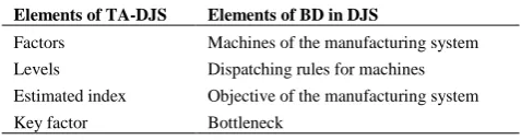
account that is not a quantitative parameter. Therefore, we cannot directly use the mentioned relation in the definitions (1) and (2) for BD. For this reason, in this study, an indirect method for BD using orthogonally and based on Taguchi Method (TA-DJS) has been applied. In this method, there is no need to calculate and . This method treats as a whole; therefore, we can obtain for each machine by using orthogonal experiment [24, 25]. The corresponding relations between the elements of Taguchi method based on orthogonal experiment (TA-DJS) and the element of BD in a DJS environment are shown in Table 1.

According to the principles of orthogonal experiment, the variation for each factors ( ) is computed by:

∑

(9) ( ) ( )

equals in Definition (1). corresponds in Definition (2). This method is an extended case of the proposed method which is extended for the studied problem in a dynamic environment and the results are brought in the following sections [24].

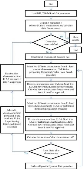
5.2. Genetic Algorithm Based on Bottleneck using Intelligent Agent (GAIA) In this section, a GA based on BR(s) is introduced by using intelligent agents for JSP which its structure and details will be discussed. 5.2.1. GAIA Structure According to Figure 1, each agent of the proposed model is developed for certain propose. The agents are:

 Adaptive Value Local Search Agent (AVLSA).  Bottleneck Local Search Agent (BLSA).  Local Search Agent (LSA).

 Elite Local Search Agent (ELSA).

5. 2. 2. GAIA Design

5. 2. 2. 1. Chromosomes Representation The first step in using GA is to represent the problem’s solutions in the form of a chromosome [26].

TABLE 1. Corresponding relations between TA-DJS and BD

Elements of BD in DJS Elements of TA-DJS

Machines of the manufacturing system Factors

Dispatching rules for machines Levels

Objective of the manufacturing system Estimated index

Considering criteria such as minimum space and time requirement is highly important due to complex computation of the problem and avoidance of creation of infeasible chromosomes in the design of the chromosomes [17, 27].

In the proposed GA, a two-dimensional

chromosome is utilized. This method is similar to Lee et al.[8]. For instance, the array (3 2 1 2 3 1 1 2) as shown in Figure 2 indicates a sample solution for the problem of Figure 3 in this representation, 1 represents job of , Figure 1. The framework of the genetic algorithm with intelligent agents

Start

Load DJS, TM-DJS and GA parameters

Construct population P (Greate N initial chromosomes and calculate

their fitness values)

Generation span satisfied

End Show results

Select two different chromosomes from P; Send selected chromosomes to DVLSA for performing DynamicallyValue Local Search

procedure

Receive chromosomes from DVLSA; Send it to LSA for performing Local Search procedure; Calculate new chromosomes fitness values and

insert it into P as approved

P has ‘Best’ elite chromosomes

Perform Operator Dynamic Rate procedure Select two different chromosomes from P; Send

selected chromosomes to BLSA for performing BottleneckLocalSearch procedure

Receive chromosomes from BLSA; Send it to LSA for performing LocalSearch procedure; Calculate new chromosomes fitness values and

insert it into P as approved

Calculate the number of elite chromosomes in P Select elit

chromosome from population P and

send it to ELSA for performing Elite Local Search

procedure Receive elite chromosome from ELSA and insert it into P as approved

Insert initial crosover and mutation rate

Yes

No

Yes

and so on. includes three operations, thus the number of repeating 1 in the chromosome is 3 times.

Layer Name

Sequence Layer

2 1 1 3 2 1 2 3

Assignment Layer

3 3 2 2 2 1 1 1

Figure 2. Chromosome Representation sample in proposed GA

The above figure is a sample solution for the following problem:

Operation Job

Figure 3. DJS with 3 job

5. 2. 2. 2. Initial Population In the proposed GA in order to avoid premature convergence, no heuristic method is used for generating initial population.

5. 2. 2. 3. Fitness Function In the GA, for evaluating the chromosomes, a certain index called fitness function is used.

Offspring 1 1 2 1 3 3 2 1 2 4 4

Parent 1 1 3 1 2 2 2 1 3 4 4

First subset{ و }Second subset{ و }

Parent 2 4 2 3 4 1 3 2 1 2 1

Offspring 2 1 2 3 1 1 3 2 4 2 4

Figure 4.POX Crossover1

Parent 1 1 2 2 1 2 3 3 1

Parent 2 3 2 1 1 1 2 2 3

Offspring 1 3 3 1 1 1 2 2 2

Offspring 2 2 1 2 1 2 3 3 1

Figure 5.Two Point Crossover1

5. 2. 2. 4. Genetic Operators

5. 2. 2. 4. 1. Crossover Operators

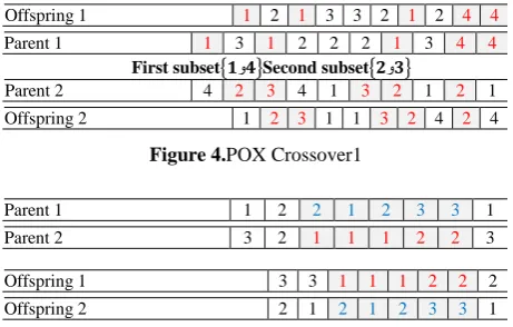
A) Crossover in Sequence Layer In the GAIA, two operators of POX and two-point operator in a combination form and with the rate of has been used. Crossover Type 1 In this crossover, two subsets of jobs are randomly selected. Then each gene from first parent belonging to the first subset is exactly transferred

to the first offspring and the other genes of the first offspring are selected from second parent belonging to the second subset (Figure 4).

Crossover Type 2 In this method, two numbers are randomly gained as cut points. Afterwards, the section between the two cut points for the two parents is swapped and then the sides for each of the offsprings are given values from parents in a way that no repetition occurs. After that, the machine’s assigned layer is also automatically adapted with the applied changes in the operation generation layer (Figure 5).

Crossover Type 3: (Two point crossover2) This crossover operator acts the same as the crossover operator in the sequence layer (TwoPoint Crossover1) differing in that by taking advantage of the chromosome’s assigned layer (in case of positive test result for the performed crossover), both selected genes for acting as two point crossover operator are the genes assigned to the bottleneck machine.

B) Crossover in Assignment Layer (Machin Crossover) After applying each of the crossover operators in the sequence layer, the crossover operator in the assignment layer is carried out in order to maintain the chromosome’s feasibility. It is in a way that in case of positive result for the test of applying crossover operator, first the crossover operator is applied on the sequence layer of the chromosome, and then the machine’s assignment layer is also automatically adapted with the applied changes in the operation generation layer.

5. 2. 2. 4. 2. Mutation Operators

Mutation Type 1 (Mutation1_1) This method is called Swap Mutation. Prior to run this method; first, mutation probability test is performed on the candidate chromosome. Then, in case of success in this test, the mentioned chromosome will undergo mutation and the values for its two selected genes (in the sequence layer) will be swapped. In this case, the machine’s assignment layer is also adapted automatically with the applied changes in the sequence layer.

Mutation Type 2 (Mutation1_2) This method is called Insert Mutation. Prior to run this method; first, mutation probability test is carried out on the candidate chromosome. If this test is successful, the mentioned chromosome will be mutated and the value for the selected gene (in the sequence layer) will be put in its place. In this case, the machine’s assigned layer is also adapted automatically with the applied changes in the sequence layer.

mutation probability test is first done for the candidate chromosome. If this test is successful, the mentioned chromosome will be mutated and the values for the two selected genes (in the sequence layer) will be inversed. In this case, the machine’s assignment layer is automatically adapted with the applied changes in the sequence layer, as well.

Mutation Type 4 through 9 Both two sets of these mutation operators act the same as the mutation operator set in the sequence layer (Mutation 1). The only difference is that by using chromosome assignment layer (in case of positive result for mutation application test) in Mutation 2 both selected genes for performing the mutation operation are genes assigned to the bottleneck machine. However, in Mutation 3 only one of the selected genes for performing mutation operation is the gene assigned to the bottleneck machine.

5. 2. 2. 5. Stop Criteria The algorithm stops after reaching to .

5. 3. Adaptability of Operators GAIA Adaptability of GA’s operators in the amount and their scope of coverage, can act as an efficient method for improving performance and effectiveness of these approaches. Whereas, adaptability in the amount of GA’s operators prevents premature convergence of the algorithm and adaptability in the scope of coverage of the algorithm results in maximum efficiency of important resources in the studied problem (such as bottleneck resources) and also improvement in the algorithm performance in each step of its run. In the proposed GA, in the first stage, adaptability for operators’ value based on premature convergence tangent rate of the algorithm’s solutions occurs. In the second stage, adaptability in the scope of coverage for the algorithm’s operators in the first step occurs with the convergence applied on the bottleneck resources (detected in pervious run) and in the next step occurs with the convergence applied on the algorithm elites. 5. 3. 1. Adaptability of Operators in the Amount- Adaptable Value Local Search Agent (DVLSA) In the GA, two operators of classic genetic with crossover and mutation rate, compete on the way of problem convergence. Whereas, incorporating mutation operator creates variety in the population, the crossover operator forces the population to converge. Considering this fact, in arranging the GA’s parameters, it is always tried to find on optimum arrangement for probabilities of applying crossover and mutation operators (using methods such as DOE, simulation, and so on). On the other hand, we know that determining and applying constant values for probability of occurring crossover the algorithm and cause premature convergence in the algorithm. For improving the GA and avoiding

premature convergence, the technique of “changing crossover and mutation rates while running the GA” has been proposed in this study (Figure 6). In GAIA, in order to avoid premature convergence (due to greater crossover rate) and also excessive variety (owing to greater mutation rate), the crossover and mutation rate adaptively changing. In this case, in GA design, the effort has been made that the amounts of mutation increase with IR and the amount of crossover decrease with DR. If this condition does not meet, the amounts of mutation and crossover will change again to the problem’s initial amounts.

5. 3. 2. Adaptability of Operators in the Scope of Coverage

A) Bottleneck Local Search Agent (BLSA)

This procedure performs bottleneck local search on the selective chromosomes of the population (Figure 7). B) Local Search Agent (LSA)

This procedure performs local search on the selected chromosomes of the population (Figure 8).

Figure 6. DynamicValue Local Search procedure Procedure DynamicValueLocalSearch

Begin

n = number of jobs; m = number of machines;

γ Crossover Proboblity;

γ Mutation Proboblity; IR = Increase Rate DR = Decrease Rate

for i = 1 to 𝑔𝑒𝑛 do Do

Get initial solutions & ;

α = random_integer_number [1,nm];

β = random_integer_number [1,nm] , β ≠ α;

Pc&PM = random_ number [0,1];

if (P_c γ) then ′ ′ = POXCrossover ( ) and MachineCrossover ( )

d = random_integer_number [1,2];

if (d > ) then ′ ′ = TwoPointCrossover1 ( ) and MachineCrossover ( )

End if End if

if (P_M γ ) then ′ ′ = Swap Mutation ( α β)

δ δ = random_integer_number [1,2];

if (δ > ) then ′ ′ = Insert Mutation ( α β)

else if (δ > ) then ′ ′ = Inverse Mutation ( α β)

End if

if (fitness( ′) fitness( )) then ′

elseif (fitness( ′) fitness( )) then ′

End if

if (“convergency test is ok”, count(elite solutions) = min(i,nm) then γ γ D &γ γ

End if

while γ 𝐶𝑟𝑜𝑠𝑠𝑜𝑣𝑒𝑟 𝑃𝑟𝑜𝑏𝑜𝑏𝑙𝑖𝑡𝑦

End while End for

disp (min(fitness( ))

Figure 7. Bottleneck Local Search procedure

Figure 9. Elite Local Search procedure

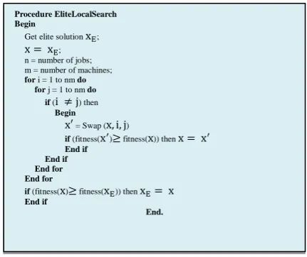
C) Elite Local Search Agent (ELSA)

This procedure performs elite local search on the elite chromosomes of the population (Figure 9).

6. DESIGN AND ADMINISTER OF NUMERICAL TESTS

6. 1. Method of Selection/ Production of Sample Problems In this section, the performance of the heuristic solving method for sub problem of bottleneck detection (TA-DJS) and GA with intelligent agents (GAIA) using different sample problems has been evaluated. These sample problems incorporate different classes of standard JSP problems such as FT test problems created by Fisher and Thompson (1963), LA test problems created by Lawrence (1984), and ORB test problems created by Applegate and Cook (1991). Simulation details for each sample (such as number of machines, jobs, operations, and process time for each operation as well as, process route) are placed in the following route:

http://people.brunel.ac.uk/~mastjjb/jeb/orlib/files/jobshop1.txt

In the first step in order to analyse TA-DJS performance, JS scheduling benchmark problems including different sizes of operation from 50, 75, 100, 150, 200, and 300. The estimation index includes . Dispatching rules for this index include FCFS, LPT, LOR, MWR, SPT, LWR, MOR, WINQ, and NINQ [28]. Furthermore, the selected orthogonal array based on 9 selected estimated indexes include (or _{). In the second step, in order to analyse GAIA} operation, all three sets of job shop scheduling benchmark problems is used. In addition, the values for GAIA parameters are as the Table 2.

Figure 8. Local Search procedure Procedure BottleneckLocalSearch

Begin

γ Crossover Proboblity;

γ Mutation Proboblity;

Get initial solutions _s & _s ;

s ;

s ; n = number of jobs; m = number of machines;

𝜗 = number of bottleneck machine;

α = random_integer_number [1,nm];

β = random_integer_number [1,nm] , β ≠ α;

Pc PM = random_ number [0,1];

if (P_c γ) then ′ ′ = POXCrossover ( ) and

MachineCrossover ( )

d = random_integer_number [1,2];

if (d > ) then ′ ′ = TwoPointCrossover2 ( 𝜗) and

MachineCrossover ( )

elseifthen ′ ′ _{= TwoPointCrossover1 ( ) and}

MachineCrossover ( )

End if End if

if (PM γ) then

δ δ,δ ,δ4,δ5,δ6 = random_integer_number [1,2];

if (δ > ) then ′ ′ = Swap Mutation2 ( α β 𝜗)

else if (δ > ) then ′ ′ = Insert Mutation2 ( α β 𝜗)

else if (δ > ) then ′ ′ = Inverse Mutation2 ( α β 𝜗)

else if (δ₄> ) then ′ ′ = Swap Mutation3 ( α β 𝜗)

else if (δ₅> ) then ′ ′ = Insert Mutation3 ( α β 𝜗)

else if (δ₆> ) then ′ ′ = Inverse Mutation3 ( α β 𝜗)

End if

if (fitness( ′) fitness( )) then ′

elseif (fitness( ′) fitness( )) then ′

End if

if (fitness( ) fitness(_s )) then _s

elseif (fitness( ) fitness( _s )) then _s

End if End.

Procedure LocalSearch Begin

Get solution S;

_S;

n = number of jobs; m = number of machines; for i = 1 to nm do

for j = 1 to nm do if ( ≠ ) then

Begin

′ = Swap ( )

if (fitness( ′) fitness( )) then ′ End if

End if End for End for

if (fitness( ) fitness( S)) then S

End if End.

Procedure EliteLocalSearch Begin

Get elite solution _E;

E; n = number of jobs; m = number of machines;

for i = 1 to nm do

for j = 1 to nm do

if ( ≠ ) then

Begin

′ = Swap ( )

if (fitness( ′) fitness( )) then ′

End if End if End for End for

if (fitness( ) fitness( _E)) then _E

End if

6. 2. The TA-DJS Results For performance analysis of BD methods, the SBD method has more reliability than the other common methods of BDP [5]. Apart from that, this method can present excellent result for DJSP [20]. Therefore, in this study, we compare the performance of the proposed TA-DJS method with the performance of MWL, BDOE, and SBD methods in the BDP. In the SBD method, we should calculate the optimal schedules before computing the machine active period. To compare the results, we suppose that the entrance time of the jobs to the shop is zero. All other parameters are similar to (1) and (11) references [7, 15]. In this section, the results from simulation are presented. For this reason, TA-DJS performance (in two-status dynamic and static) is compared to a prior-to- run BD called BD-OE and a posterior-prior-to-run BDcalled SBD and MWL methods. The results are shown in Tables 3, 4 and 5. According to the studies of Hinckeldeyn et al. (2014), there are various bottleneck

counter measures such as scheduling solution, targeted source increase, increase of resource flexibility, process important, reduce workload of BR, and bottleneck oriented counter pricing [3]. Among these, 75% of the investigated researches by Hinckeldeyn et al. (2014) are carried counter out using scheduling solution approach as the bottleneck counter measures are [3]. Accordingly, in this study, in order to analyse the results of differences for the 3 mentioned methods, the MODJS with the objective of makespan and based on the detected bottleneck, has been solved and the results are brought about in Table 6.

TABLE 2. The GAIA Parameters

γ_2 IR DR

100 100 0.95 0.10 0.001 0.001

TABLE 3. BD results for small scale problems

Problem’sNumber Problem’sSize(nm)

Bottleneck Resource(s) Computational Time(s)

DynamicTA-DJS

StaticTA-DJS

BD-OE

SBD MWL

DynamicTA-DJS

StaticTA-DJS

SBD

LA 01 105 5 5 5 5 5 0.30 0.30 7.50

LA 02* 105 5 1 1 4 4 0.30 0.30 43.70

LA 03 105 1 2 2 2 2 0.31 0.31 47.90

LA 04* 105 1 5 1,3,5 1,3 5 0.30 0.30 46.60

LA 06 155 1 1 1 1 1 0.55 0.55 56.20

LA 07 155 1 1 1 1 1 0.55 0.55 55.60

LA 08* 155 3 4 3 5 5 0.55 0.55 65.30

LA 09 155 2 2 2 2 2 0.54 0.55 47.40

Instances with * express that the bottlenecks detected by the three methods are different.

TABLE 4. BD results for median scale problems

Problem’sNumber Problem’sSize(nm)

Bottleneck Resource(s) Computational Time(s)

DynamicTA-DJS

StaticTA-DJS

BD-OE

SBD MWL

DynamicTA-DJS

StaticTA-DJS

SBD

LA 16* 1010 3 3 1,3 1,3 1 5.62 5.64 112.60

LA 17 1010 4 4 4 4 4 5.54 5.51 134.90

LA 18 1010 2 1 1 1 1 5.55 5.56 171.50

LA 19* 1010 3 10 2 7 7 10.14 9.88 263.60

LA 21 1510 10 10 10 10 1 9.81 9.96 240.60

LA 22 1510 5 5 5 5 8 9.85 9.98 208.10

LA 23 1510 7 7 7 7 7 9.86 9.96 251.60

LA 24* 1510 10 2 10 10 10 5.62 5.64 112.60

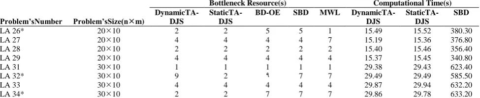
TABLE 5. BD results for large scale problems

Problem’sNumber Problem’sSize(nm)

Bottleneck Resource(s) Computational Time(s)

DynamicTA-DJS

StaticTA-DJS

BD-OE SBD MWL

DynamicTA-DJS

StaticTA-DJS

SBD

LA 26* 2010 2 2 5 5 1 15.49 15.52 380.30

LA 27 2010 4 4 4 4 7 15.19 15.36 376.80

LA 28 2010 2 2 2 2 2 15.40 15.46 356.40

LA 29 2010 4 4 4 4 4 15.37 15.45 340.80

LA 31 3010 1 1 1 1 1 29.38 29.43 623.40

LA 32* 3010 9 2 9 7 7 29.49 29.49 585.50

LA 33 3010 4 4 4 4 4 29.87 29.94 632.20

LA 34* 3010 2 2 7 7 7 29.86 29.78 633.20

TABLE 6.The scheduling results using the BD by the 3 methods

Problem’s Number Problem’s Size(nm)

Bottleneck Resource(s) Computational Time (second)

Static TA-DJS

BD-OE SBD Static

TA-DJS

BD-OE SBD

LA 02 105 1 1 4 821.8 821.8 870.0

LA 04 105 5 5 3 702.6 702.6 760.4

LA 08 105 4 3 5 902.0 1007.4 1137.9

LA 16 105 3 1 3 1088.0 1102.3 1088.0

LA 19* 155 10 2 7 962.0 951.0 1060.0

LA 24 155 2 10 10 1126.6 1354.0 1354.0

LA 26 155 2 5 5 1488.0 1716.3 1116.3

LA 32 155 2 9 7 1996.0 2593.8 2540.9

Instances with * express that the bottlenecks detected by the three methods are different.

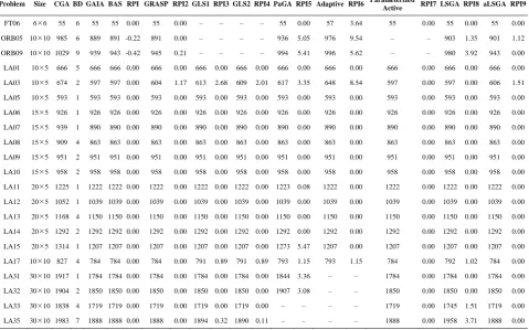
TABLE 7. Experimental results on FT, ORB and LA instances.

Problem Size CGA BD GAIA BAS RPI GRASP RPI2 GLS1 RPI3 GLS2 RPI4 PaGA RPI5 Adaptive RPI6 Parameterized

Active RPI7 LSGA RPI8 aLSGA RPI9

FT06 66 55 6 55 55 0.00 55 0.00 – – – – 55 0.00 57 3.64 55 0.00 55 0.00 55 0.00

ORB05 1010 985 6 889 891 -0.22 891 0.00 – – – – 936 5.05 976 9.54 – – 903 1.35 901 1.12

ORB09 1010 1029 9 939 943 -0.42 945 0.21 – – – – 994 5.41 996 5.62 – – 980 3.92 943 0.00

LA01 105 666 5 666 666 0.00 666 0.00 666 0.00 666 0.00 666 0.00 666 0.00 666 0.00 666 0.00 666 0.00

LA03 105 674 2 597 597 0.00 604 1.17 613 2.68 609 2.01 617 3.35 648 8.54 597 0.00 597 0.00 606 1.51

LA05 105 593 1 593 593 0.00 593 0.00 593 0.00 593 0.00 593 0.00 593 0.00 593 0.00 593 0.00 593 0.00

LA06 155 926 1 926 926 0.00 926 0.00 926 0.00 926 0.00 926 0.00 926 0.00 926 0.00 926 0.00 926 0.00

LA07 155 939 1 890 890 0.00 890 0.00 890 0.00 890 0.00 890 0.00 890 0.00 890 0.00 890 0.00 890 0.00

LA08 155 909 4 863 863 0.00 863 0.00 863 0.00 863 0.00 863 0.00 863 0.00 863 0.00 863 0.00 863 0.00

LA09 155 951 2 951 951 0.00 951 0.00 951 0.00 951 0.00 951 0.00 951 0.00 951 0.00 951 0.00 951 0.00

LA10 155 958 2 958 958 0.00 958 0.00 958 0.00 958 0.00 958 0.00 958 0.00 958 0.00 958 0.00 958 0.00

LA11 205 1225 1 1222 1222 0.00 1222 0.00 1222 0.00 1222 0.00 1223 0.08 1222 0.00 1222 0.00 1222 0.00 1222 0.00

LA12 205 1052 1 1039 1039 0.00 1039 0.00 1039 0.00 1039 0.00 1039 0.00 1039 0.00 1039 0.00 1039 0.00 1039 0.00

LA13 205 1168 4 1150 1150 0.00 1150 0.00 1150 0.00 1150 0.00 1150 0.00 1150 0.00 1150 0.00 1150 0.00 1150 0.00

LA14 205 1292 2 1292 1292 0.00 1292 0.00 1292 0.00 1292 0.00 1292 0.00 1292 0.00 1292 0.00 1292 0.00 1292 0.00

LA15 205 1314 1 1207 1207 0.00 1207 0.00 1207 0.00 1207 0.00 1273 5.47 1207 0.00 1207 0.00 1207 0.00 1207 0.00

LA17 1010 827 4 784 784 0.00 784 0.00 791 0.89 791 0.89 793 1.15 793 1.15 784 0.00 792 1.02 784 0.00

LA31 3010 1917 1 1784 1784 0.00 1784 0.00 1784 0.00 1784 0.00 1844 3.36 – – 1784 0.00 1784 0.00 1784 0.00

LA32 3010 1904 2 1850 1850 0.00 1850 0.00 1850 0.00 1850 0.00 1907 3.08 – – 1850 0.00 1850 0.00 1850 0.00

LA33 3010 1838 4 1719 1719 0.00 1719 0.00 1719 0.00 1719 0.00 – – – – 1719 0.00 1745 1.51 1719 0.00

LA35 3010 1983 7 1888 1888 0.00 1888 0.00 1894 0.32 1890 0.11 – – – – 1888 0.00 1958 3.71 1888 0.00

TABLE 8. Average RPI

Algorithm NIS

Mean RPI

OA GAIA Improvement

GAIA

GRASP 21 0.07 0.06 -0.01

GLS1 18 0.22 0.22 0.00

GLS2 18 0.17 0.17 0.00

PaGA 19 1.42 1.45 0.04

Parameterized

Active 19 1.68 1.72 0.04

Adaptive 17 0.00 0.00 0.00

LSGA 21 0.55 0.58 0.03

aLSGA 21 0.13 0.16 0.03

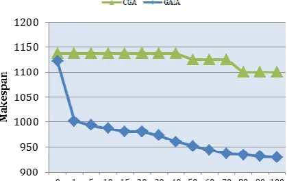
Figure 10. Makespan versus generation for CGA and GAIA

Figure 11. Makespan versus generation for CGA and GAIA for FT10 instance

6. 3. The GAIA Results In order to determine the performance of the GAIA, results are compared with other algorithms. A summary of experimental results is given in Tables 7–8. Tables list problem name, problem size, and GAIA in two stages of dynamic and static. In the section for comparing GAIA results in static state, the mentioned tables, as well as, incorporating GAIA results in static state and the Best Available Solution (BAS) from running the algorithms utilized for solving the research problem include as index called Relative Percentage of Improvement (RPI) by using the following equation:

P

(10)

A comparison between average RPI obtained by proposed approach and the other algorithms are given in Table 8. This table shows the number of instances solved (NIS), and the average relative percent improvement (RPI) for the GIAI, and for the other algorithms (OA) listed in the table. The column named improvement shows the reduction of RPI obtained by the GAIA with respect to each of the other algorithms. For showing the behavior of the convergence point, the GAIA is compared with simple GA. The algorithms applied on some problem instances during various generations and the average makespan of the best schedules obtained are shown in Figures 10 and 11.

7. SENSITIVITY ANALYSIS

7. 1. Analyzing the Performance of TA-DJS According to the results revealed in Tables 3, 4, 5 and 6, The bottleneck’s conforming rate:

 in the two methods of TA-DJS and SBD for different scale problems of DJS is up to 63%.  in the two methods of TA-DJS and BD-OE for

small, medium, and large scale problems of DJS is up to 88%, 63%, and 63% respectively. In addition,

the bottleneck’s conforming rate for in the two methods of TA-DJS and BD-OE for problems to different scales of DJS is generally up to 71%.  The results from solving scheduling problem based

on the detected bottleneck for variations indicate significant in 89% of problems.

7. 2. Analysis of GAIA Performance According to the inserted results in the Tables 2, 3 and 4, it is observed that:

 Improvement rate of the BAS for sample problems with different scales for DJS in the ORB class, with objective function is up to %78 (7 better samples among 9 samples).

 Improvement rate of the BAS for sample problems with different scales for DJS in the LA class, with objective function is up to %20.

According to Table 5, it is observed that the proposed algorithm has created a significant improvement in the quality of solutions, in comparison with almost all other algorithms (except Parameterized Active Algorithm). Diagrams (13) and (14) illustrate the effect of implementing GAIA and classic GA methods on the sample problems of LA29 and FT10. As illustrated in these diagrams, the convergence rate in GAIA is more than that of classic GA and solution resulted from GAIA in the number of different generation possess shorter lengths compared to those of classic GA. Hence, taking advantage of intelligent agents during running the GA increases convergence rate and improve in quality of these algorithms.

8. CONCLUSION REMARKS

environments are such available fields for further research.

9. REFERENCES

1. Asadzadeh, L., "A local search genetic algorithm for the job shop scheduling problem with intelligent agents", Computers & Industrial Engineering, Vol. 85, (2015), 376-383.

2. Zhang, R. and Wu, C., "Bottleneck machine identification method based on constraint transformation for job shop scheduling with genetic algorithm", Information Sciences, Vol. 188, (2012), 236-252.

3. Hinckeldeyn, J., Dekkers, R., Altfeld, N. and Kreutzfeldt, J., "Expanding bottleneck management from manufacturing to product design and engineering processes", Computers and Industrial Engineering, Vol. 76, (2014), 415-428.

4. Gupta, M., Ko, H.-J. and Min, H., "TOC-based performance measures and five focusing steps in a job-shop manufacturing environment", International Journal of Production Research, Vol. 40, No. 4, (2002), 907-930.

5. Bruker, P., Jurisch, B. and Sievers, B., "Discrete applied mathematics'', The Journal of Combinatorial Algorithms, Informatics and Computational Sciences, Vol. 49, (1994), 107-112.

6. Carlier, J. and Pinson, E., "An algorithm for solving the job-shop problem", Management Science, Vol. 35, No. 2, (1989), 164-176.

7. Brandimarte, P., "Exploiting process plan flexibility in production scheduling: A multi-objective approach", European Journal of Operational Research, Vol. 114, No. 1, (1999), 59-71.

8. Lee, Y.H., Jeong, C.S. and Moon, C., "Advanced planning and scheduling with outsourcing in manufacturing supply chain",

Computers & Industrial Engineering, Vol. 43, No. 1, (2002), 351-374.

9. Tay, J.C. and Ho, N.B., "Evolving dispatching rules using genetic programming for solving multi-objective flexible job-shop problems", Computers & Industrial Engineering, Vol. 54, No. 3, (2008), 453-473.

10. Gao, J., Gen, M. and Sun, L., "Scheduling jobs and maintenances in flexible job shop with a hybrid genetic algorithm", Journal of Intelligent Manufacturing, Vol. 17, No. 4, (2006), 493-507.

11. Moreno-Torres, J.G., Llora, X. and Goldberg, D.E., "Binary representation in gene expression programming: Towards a better scalability", in Intelligent Systems Design and Applications, ISDA'09. Ninth International Conference on, IEEE, (2009), 1441-1444.

12. Dagli, C. and Sittisathanchai, S., "Genetic neuro-scheduler: A new approach for job shop scheduling", International Journal of Production Economics, Vol. 41, No. 1, (1995), 135-145.

13. Ghedjati, F., "Genetic algorithms for the job-shop scheduling problem with unrelated parallel constraints: Heuristic mixing method machines and precedence", Computers & Industrial Engineering, Vol. 37, No. 1, (1999), 39-42.

14. Kurz, M.E. and Askin, R.G., "Scheduling flexible flow lines with sequence-dependent setup times", European Journal of Operational Research, Vol. 159, No. 1, (2004), 66-82. 15. Kurz, M.E. and Askin, R.G., "Comparing scheduling rules for

flexible flow lines", International Journal of Production Economics, Vol. 85, No. 3, (2003), 371-388.

16. Tay, J.C. and Wibowo, D., "An effective chromosome representation for evolving flexible job shop schedules", in Genetic and Evolutionary Computation–GECCO, Springer, (2004), 210-221.

17. Abbasian, M. and Nahavandi, N., "Minimization flow time in a flexible dynamic job shop with parallel machines", Journal of Sharif, in press, (2010).

18. Abbasian, M. and Nahavandi, N., "Minimization flow time in a flexible dynamic job shop with parallel machines", Tehran, Tarbiat Modares University, Engineering Department of Industrial Engineering, Master of Science Thesis, (2009). 19. Goldberg, D.E., "Genetic algorithms in search optimization and

machine learning, Addison-wesley Reading Menlo Park, Vol. 412, (1989).

20. Ho, N.B., Tay, J.C. and Lai, E.M.K., "An effective architecture for learning and evolving flexible job-shop schedules",

European Journal of Operational Research, Vol. 179, No. 2, (2007), 316-333.

21. Amiri, M., Falah, J.S. and Salehi, S.J., "A genetic algorithm approach for statistical multi-response models optimization: A case study", (2009).

22. Abbasian, M. and Nahavandi, N., "Solving multi-objective flexible dynamic job-shop scheduling problem with parallel machines", International Journal of Industrial Engineering of Production Research, Vol. 21, No. 3, (2011).

23. Verma, A., Llora, X., Venkataraman, S., Goldberg, D.E. and Campbell, R.H., "Scaling ecga model building via data-intensive computing", in Evolutionary Computation (CEC), IEEE Congress on, IEEE, (2010), 1-8.

24. Zhai, Y., Sun, S., Wang, J. and Niu, G., "Job shop bottleneck detection based on orthogonal experiment", Computers & Industrial Engineering, Vol. 61, No. 3, (2011), 872-880. 25. Zhai, Y., Sun, S., Wang, J. and Wang, M., "An effective

bottleneck detection method for job shop", International Conference on Computing, Control and Industrial Engineering, (2010), 198-201.

26. Park, B.J., Choi, H.R. and Kim, H.S., "A hybrid genetic algorithm for the job shop scheduling problems", Computers & Industrial Engineering, Vol. 45, No. 4, (2003), 597-613. 27. Abbasian, M., Nosratabadi, H. and Fazlollahtabar, H.,

Solving the Dynamic Job Shop Scheduling Problem using Bottleneck and Intelligent

Agents based on Genetic Algorithm

N. Nahavandi, S.H. Zegordi, M. Abbasian

Faculty of Industrial and Systems Engineering, Tarbiat Modares University, Tehran, Iran

P A P E R I N F O

Paper history:

Received 27December 2015

Received in revised form 19February 2016 Accepted 03March 2016

Keywords: Dynamic Job Shop Genetic Algorithm Unmaturity Convergency Inteligent Agent Theory of Constraint

Bottleneck Resource(s) Detection

هديكچ

نامز هلئسم ( ایوپ یهاگراک راک یدنب DJS

هدیچیپ زا یکی ) نامز تلااح نیرت

هب نیشام یدنب یم رامش

هتسد زا هلئسم نیا .دور

لئاسم NP-Hard هب

یم رامش شور نونکات هک دور .تسا هدش هئارا نآ لح یارب یددعتم یراکتباارف و یراکتبا یاه

وگلا متیر ( کیتنژ یاه GA

شور نیا هلمج زا ) هب هک تساه

تیقفوم روط عقاو هدافتسا دروم لئاسم زا هتسد نیا لح یارب یزیمآ

هدش شور زا هتسد نیا رد هتبلا .دنا باوج تیفیک دوبهب ،متیروگلا سردوز ییارگمه زا بانتجا مه زونه اه

اهنآ یراوتسا زین و اه

شلاچ ثحابم هلمج زا تسه زیگنارب

.دن یاهرگلمع ییایوپ GA

یم ششوپ تحت ۀزوح و رادقم رد یدرکیور ناونع هب دناوت

رد .دیامن لمع آراک GA

( یداهنشیپ GAIA ییارگمه بیش خرن ساسا رب متیروگلا یاهرگلمع رادقم رد ییایوپ :لوا ماگ رد )

یم یور متیروگلا سردوز اهرگلمع ششوپ تحت ۀزوح رد ییایوپ :مود ماگ رد سپس .دهد

ی GA عبانم یور رب تسخن ،

یم ییاسانش ادتبا رد هک( یهاگولگ باوج یور رب یدعب ۀلحرم رد سپس و هدش لامعا )دنوش

یم یور هبخن یاه رما نیا .دهد

هزوح رب متیروگلا زکرمت هب رجنم لمتحم یاه

یم هلئسم باوج یاضف زا یرت زا کیتاتسا تلاح رد متیروگلا جیاتن ۀسیاقم .دوش

اب هلئسم شور زا لصاح جیاتن .تسا یداهنشیپ درکیور یلااب ییآراک زا یکاح ،قیقحت تایبدا رد دوجوم یاه