A New Technique based on Strain Energy for Correction of Stress-strain Curve

Please cite this article as: G. H. Majzoobi and F. Fariba, A New Technique Based on Strain Energy for Correction of Stress-Strain Curve. International Journal of Engineering (IJE) Transactions B: Applications Vol. 27, No. 8, (2014): 1287-1296

International Journal of Engineering

J o u r n a l H o m e p a g e : w w w . i j e . i r

A New Technique based on Strain Energy for Correction of Stress-strain Curve

G. H. Majzoobi*a, _{F. Fariba}b

a _{Mechanical Engineering Department, Bu-Ali Sina University, Hamedan, Iran} b _{Islamic Azad University, Takestan Branch, Takestan, Iran}

P A P E R I N F O

Paper history:

Received 18 November 2013

Received in revised form 15 January 2014 Accepted in 06 March 2014

Keywords: Stress-strain curve, Correction factor Strain energy External work Numerical simulation

A B S T R A C T

Tensile stress-strain curve is of high importance in mechanics of materials particularly in numerical simulations of material deformations. The curve is usually obtained by experiment, but is limited by the necking phenomenon. Engineering stress-strain curve is converted to true stress-strain curve through simple formulas. The conversion, however, is correct up the point of necking. From this point on, the curve should be corrected taking account of stress triaxiality. Over the past several decades, a number of methods such as Bridgeman correction technique have been proposed. In this investigation a new technique based on strain energy in introduced. Strain energy is assumed to be equal to the external work in tensile test. The energy method is compared with different approaches such as Bridgeman-Leroy, Bridgeman, Davidenkov, Siebel and optimization aided numerical simulation. The results indicate that the energy method prediction is very close to numerical simulation, but at the same time it does not differ too significantly from the other approaches studied in this investigation.

doi: 10.5829/idosi.ije.2014.27.08b.15

NOMENCLATURE

a Diameter of neck section σ ,σ ,σθ Longitudinal, radial, tangential stresses σ Equivalent/corrected stress R Curvature radius dε Equivalent strain W External work

CF Correction factor dε , dε , dεθ Longitudinal, radial, tangential strains U Elastic strain energy ε Necking strain U Plastic strain energy r = f(z) Neck profile function

σ Necking stress H Head loss energy K, n Power law material model parameter

ε True strain u Strain energy density OBJ(x, y) Objective function

σ True stress W External work done from start point to final u , u Displacement in the r and z direction

S Engineering stress U Strain energy from start to final point A Initial area

e Engineering strain U Strain energy in un-neck part of specimen V Initial volume

ε Average longitudinal strain U Strain energy in neck part of specimen V Un-neck volume of specimen

L Initial length u Strain energy density from start to necking L Final length

A Final area u Strain energy density of element

1. INTRODUCTION1

True stress-strain curve represents the yield surface of a material and is an essential requirement in the theory of plasticity, particularly in simulations of large non-linear plastic deformations. True stress-strain curve (TSS) is obtained from engineering stress-strain curve (ESS) which in turn is computed from load-displacement

1_{* Coresponding Author’s Email: gh_majzoobi@basu.ac.ir (G. H.} Majzoobi)

It seems that the first investigation was performed by

Bridgeman [1] who presented a comprehensive analysis of stress and strain in neck area and proposed a correction factor (CF), based on neck geometry, as follows:

= 1 + (1 + ) , = .σ (1)

In this correction method, the ratio R/a plays an important role in computing the correction factor. R and a are the radii of the neck curvature and the narrowest neck section, respectively. This ratio must be computed during tensile tests at some time intervals. This is a tedious and time consuming task which is accompanied by approximations which arise from simplifying assumptions made by Bridgeman in his theory. Later, Davidenkov and Spiridonova [2] and Siebel and Schwaigere [3] separately proposed different relations for correction factors as follows:

1 1 ( / 2 ) CF

a R

 

=  ₊ 

 

(Davidenkov),

1 1

1 ( / 4 ) CF

a R

 

=  ₊ 

 

(Siebel)

(2)

The correction factors proposed by Bridgeman, Davidenkov and Siebel are known as classic relations. One of the main difficulties associated with the classic relations is the measurement of radius of curvature of the neck during tensile test. In 1981 Leroy [4] proposed a relation for calculation of the neck curvature radius. The relation is expressed in terms of the current strain, , and the strain at the onset of necking, , as follows:

= 1.1(ε − ε ) (3)

Leroy et al. [4] have shown that for a wide range of metals, the approximation due to the use of Equation (3) for computing the ratio R/a is less than 25%. By appearance of finite element method in mechanical engineering, researcher employed finite element codes and programming to model the necking phenomenon. Finite element capabilities enabled the researchers to correct the stress-strain curves and investigate stress and strain distributions in the neck area. Niddleman [5] used finite element method for modeling the necking phenomenon based on boundary problems and plasticity. In 1998 Brunig [6] analyzed cylindrical specimens under tension using large deformation finite element analysis. Niordson and Redanz [7] modeled necking in a thin rectangular plate using the strain gradient plasticity theory already introduced by Fleck and Hutchinson [8]. Their model is based on the delay between maximum load and the onset of necking. Koc and Stok [9] analyzed stress distribution in neck area using Abaqus software and introduced the inverse method for correction of stress-strain curve. He also, optimized the difference between load-displacement curves from test and numerical simulation for

stress-strain curve correction. Tang and Lee [10] analyzed necking in a bar under simple tension using a coupled strain hardened and damage models. He studied the effect of damage model on the necking phenomenon. Since necking is inherently a consequence of damage (void growth and coalescence), coupling of material model with damage model can significantly improve the correction techniques. Ling [11] introduced a special function for describing the relation between stress and strain after necking. He obtained the function by numerical simulation using Abaqus. His analysis was based on optimization of the difference between experimental and numerical load-displacement curves. A number of creative correction techniques have been proposed by researchers such as Mirone [12]. His method is applicable to a wide range of metals. Mirone [12] presented some criteria independent of the type of material and introduced relations for stress-strain correction. Coppieters et al. [13] presented an alternative method to identify the post-necking hardening behavior of sheet metal. His method is based on the minimization of the difference between the internal and external work in the necking zone during a tensile test. Eduardo [15] presented an experimental-numerical methodology to derive the elastic and hardening parameters which characterize the material response. Yang and Cheng [16] introduced a damage mechanics based model to describe the progressive deterioration of materials prior to initiation of macro cracks. Majzoobi et al. [17, 18] identified the constants of Johnson–Cook, power law and Zerilli–Armstrong models in tension and compression using a combined experimental/ numerical/ optimization approach. The models take account of correction indirectly and there is no need for computing the correction factor directly. Gromada et al. [19] analyzed and estimated the accuracy of the well-known classical formulae for correction stress-strain curve.

segment corresponds to only uniform deformations. The second segment is assumed to be linear, = + , begining from the point of necking onset and terminating at the point of fracture. The values of K and n are determined from a simple curve fitting to true stress-strain curve. The correction of stress-strain curve should in fact be applied to the line segment. Therefore, constants A and B are identified through energy and classic methods mentioned above. These trends can be applied to a considerable number of metals stress-strain curve. Nevertheless, as will be explained in the next sections, there is no limit for the kind of stress-strain trend used in energy method.

2. THEORY OF ENERGY METHOD

Engineering stress-strain curve obtained from load-displacement curve can be converted to true stress-strain diagram through the relations [11]:

σ= S(1 + e)ε= Ln(1 + e) (4)

in which e, , S and denote engineering strain, true strain, engineering stress and true stress, respectively. Equations (4) hold up to the point of necking. True strain can also be computed from the relation [12]:

ε = Ln = Ln = 2Ln (5)

in which A, L and D are cross sectional area, length and diameter, respectively. The diameter, D, of the specimen must be determined from tensile test using a speed camera along with some graphical manipulation known as image processing. This technique is used to determine the diameter of specimen which in turn is used for calculation of stress and strain (strain is calculated from Equation (5) and stress is computed from P/A). In this technique, some marks are printed on the specimen before deformation. The marks are displaced during deformation. The displacement of the marks is recorded using a camera with 30 fps (frames per second). Also, the diameter, profile and length of the specimen’s neck are measured from the recorded images of the specimen versus time. The diameter is used for calculation of true stress and strain and the neck profile is used for calculation of R which is needed for computing correction factor in Bridgeman and some other methods. The subscripts 0 and f also denote the initial and final values of the dimensions, respectively. The stress-strain curve obtained using Equations (4) and (5) must be corrected after the point of necking. As a matter of fact, stress triaxiality at neck area necessitates the stress-strain diagram to be corrected. Effective stress and strain for an axisymmetric analysis which is the case for tension of a cylindrical specimen are given by [11]:

=_√ [( − ) + ( − ) + ( − )]/ ₍₆₎

dε =√ [(dε −dε) + (dε −dε ) + ( − )]/ ₍₇₎

where r, z and , are radial, longitudinal and tangential directions of the stress and strain components, respectively. From the volume constancy in plastic deformation we have [11]:

dε + dε + dε = 0 (8)

In axisymmetric deformation we can write:

dε =−2dε =−2dε (9)

Substituting Equation (9) in Equation (7), we get:

= (10)

The corrected stress-strain curve can be presented in different forms. In some cases, it is displayed only in graphical form. However, in most cases, the corrected curve is described by empirical equations such as Holomon, Ludwick constitutive equations, etc. It can be assumed that for a conservative system (neglecting the effects of friction and hysteresis) the external work which is the area under the load-displacement curve is equal to the internal energy which is related to the area under the stress-strain curve. This assumption can be expressed as follows:

= + + (11)

in which is the external work, H the loss of energy due to friction, etc. and and are elastic and plastic strain energy, respectively. If the effect of strain energy which is small compared to plastic energy and the loss of energy are neglected, then we will have:

= = (12)

where, the external work can be expressed by [13]:

=∫ . (13)

P and represent the load and displacement in tensile test, respectively. For more accuracy, extensometer is used for measuring the elongation of the specimen. On the other hand, strain energy per unit volume is defined by [14]:

u =∫σ dε (14)

For an axisymmetric tensile specimen, Equation (14) can be rewritten as:

u =∫(σdε +σdε +σ dε ) (15)

Using Equation (9) we can write:

u =∫(σdε −0.5σdε −0.5σ dε ) =∫ σ −

(σ +σ ) dε

(16)

From the elementary plasticity we have[11]:

dε = σ − (σ +σ ) (17)

u =∫ dε dε =∫σ dε (18)

This equation implies that the area under the effective stress-strain curve is equal to the strain energy density in a tensile cylindrical specimen. The equation is the basis for the current investigation. The equality of the areas under engineering and true strain curve which extends to the point of necking can be proved by differentiating from Equation (4) as follows:

dε= … . .σdε= S(1 + e). = Sde (19)

Therefore, we can write:

∫_εε σdε=∫ S de ε≤ε (20)

From Equations (12), (20) and (18) one can write:

_{=∫ Sde=∫}ε _σdε

ε ε≤ε (21)

Equation (20) does not hold after necking. The reason is that each point in neck area experiences different stress and strain. Therefore, a different equation is required for describing the relation between engineering and true stress-strain curves after necking. This is accomplished using energy method in this work. The maximum stress and strain occurs in the neck area. However, the stress and strain experienced by other points located on different sections lie exactly on the same stress-strain curve. Therefore, for determining the strain energy of specimen the following equation must be used:

U =∫u. dV =∫ ∫σ dε . dV (22)

For computing the energy from Equation (22) we need to have the stress distribution within specimen. This is a difficult task. Here, a new approach is proposed for computing the strain energy as follows:

W = U (23)

where and are the external work and the strain energy of the specimen, from start till final point respectively. Strain energy can be written as:

U =∫ ∫ σ dε . dV (24)

We can divide the strain energy of specimen into two parts. Part one is the strain energy in the un-necked region where deformation is uniform. Part two corresponds to the strain energy in the neck region. We can write:

U = U + U (25)

where is the strain energy in the un-necked part and is strain energy in the neck region of the specimen. We have:

= . (26)

where is the strain energy density from 0 to the necking onset.

Figure 1. The energy of a disk type element in neck area

In order to compute the energy equation from tensile test in neck region ( ), an infinitesimal cylindrical element is considered in the neck region as shown in the figure . A key point is that equivalent stress in neck section is the same over the entire area of the section. This is one of the assumptions in Bridgeman method with the maximum error of around 0.5 percent [19]. This assumption has been used by some other researchers such as Eduardo and Celentano [15] as well and is considered in the numerical results presented in this work too. Therefore, each element can be considered as a solid disk with constant equivalent stress. For this element in neck region, the total strain energy can be written as:

dU = ∫ σ dε . dV = u . dV (27)

where is equivalent strain corresponding to the element. Also, is the strain energy density of the element that equals to area under strain-stress curve till the point of the element fracture strain. This is shown in Figure 1. The volume of the element can be expressed as follows:

V =π. r . dz (28)

where r is the radius of the element and can be expressed by r=f(z). By substituting Equation (28) into Equation(27), strain energy density of the element can be determined as follows:

dU = u .π. {f(z)} . dz (29) Therefore, the total strain energy for specimen can be written as:

=∫ = 2∫ / ∫ . . { ( )} . (30)

where is the neck length of specimen which is determined using image data obtained from tensile test. By substituting the strain energy from Equation (30) and Equation (26) into Equation (25),we get:

∫ σdε =∫ σ dε +∫ σ dε = u +∫ σ dε (32)

The second term in Equation (31),can be written:

∫ / ∫ =∫ / +∫ (33)

We can write:

∫ / u . dV = u .∫ / dV = u . V (34)

where, is the neck volume of specimen. By substituting Equation (34) into Equation (33), and using Equation (31) with volume constancy principal in plastic deformation we obtain:

U = u . V + 2∫ / ∫ σ dε .π. {f(z)} .dz (35)

Having determined the strain energy of the specimen, we can write the energy balance equation for a cylindrical specimen in tensile test as follows:

W =∫ P. dδ= U = u . V +

2∫ / ∫ σ dε .π. {f(z)} . dz (36) This equation can be used for computing the corrected stress-strain curve. For this purpose, Equation (36) must be solved by a numerical method. We assume a linear relation between stress and strain after necking (as stated before) and a second order polynomial for the profile of neck as follows:

= + (37)

= + + (38)

These assumptions are quite optional and the method presented here, can accommodate any other trends for stress-strain curve and neck profile. By substituting for and r from Equations (37) and (38) into Equation (36) we get:

∫ P. dδ= u V + 2∫ ε − ε +

B(εe−εN)+ π C1z2+ C2z + C3 2 dz

(39)

By rearranging Equation (39) in terms of A and B, we obtain:

Aπ ∫ ε − ε (C z + C z + C ) dz

+2Bπ ∫ [(ε − ε ). (C z + C z + C ) dz]

=∫ P. dδ−u . V

(40)

On the other hand, the stress-strain relation after necking can be written for the point of necking onset. Therefore, we can write:

= + (41)

From the simultaneous solution of Equations (40) and (41), the values of A and B can be determined.

3. TENSILE TEST AND SPECIMEN

Tensile tests were conducted on a 60 tons Instron testing machine. Specimens were made of steel st304 prepared

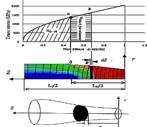
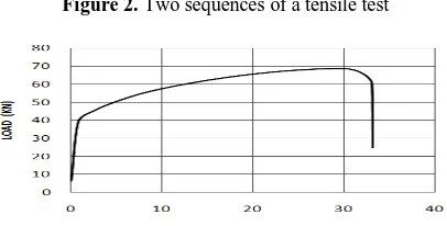
according to the standard ASTM-E8 [20]. The dog bone type specimens had a gauge length of 55 mm and a diameter of 9.86 mm. The tensile tests were carried out at 5 mm/min at room temperature. A DCR-HC32E handy cam with 30 frames per second was used to capture the deformation of specimens before and after necking. From the recorded images, the dimensions and profile of the neck were measured. The resolutions of the images were enhanced using graphical software and the required data were extracted using point detection software named as Gate Data and Digitizer. Typical deformation of marked specimens is illustrated in Figure 2. The load-displacement and stress strain curves of the specimen are shown in Figures 3 and 4, respectively. The engineering stress-strain curve, the true stress-strain diagram obtained using Equation (4) and the true stress-strain curve extracted from image processing (strain is calculated from Equation (5) and stress is computed from P/A) are illustrated in Figure 4. As the figure suggests, the two types of the true stress-strain curves are quite different after necking. In order to validate the image processing used in this work, the smallest neck area was measured from the images taken by camera and was calculated using the relation[11]:

= ( ) ₍₄₂₎

The results are illustrated in Figure 5. As the figure suggests, the results of both methods nearly coincide up to the point of necking. After necking, the two methods yield different predictions due to invalidity of Equation (42) after necking. This validates the image processing technique used in this work on one hand and confirms the invalidity of Equation (4) for computing true stress and strain after necking on the other hand. From a curve fitting to the true stress-strain curve and using a piecewise function defined by a power law followed by a line, we can easily obtain:

₌= ₊ ≤_>, _, = 1948 , _{= 1287} = 0.46_{= 767} (43)

Figure 2. Two sequences of a tensile test

Figure 4. Stress-strain curves obtained using different

approaches

Figure 5. Variation of neck cross sectional area versus time

TABLE 1. Three dimensions measured through image

processing

The length of neck region

(mm) Diameter of

unnecked region (mm) Diameter of

neck (mm) Time (s)

No neck 9.86

9.86 start

No neck 9.36

9.36 60 s

No neck 9

9 120 s

No neck 8.55

8.55 210 s

No neck 8.09

8.09 320 s

10.7 8.18

7.64 360 s

12.7 8.18

7.27 370 s

13.6 8.18

6.36 380 s

20.91 8

6.14 Fracture

The stress-strain curve obtained using Equation (43) coincides exactly with that shown in Figure 4. This illustrates the accuracy of the constants obtained from curve fitting. However, the true stress-strain shown in Figure 4 is not usable after necking and should be corrected taking account of stress triaxiality after necking. Three dimensions were measured from image processing at different times. These were: smallest neck diameter (a), diameter of specimen in uniform deformation zone (r) and the length of neck area (LN).

These dimensions will be used for numerical simulations and also for energy method which is the main subject of this work. The results are given in Table 1.

4. INPLEMENTATION OF ENERGY METHOD

The calculation of strain energy could be performed in two steps, before and after necking. The following information is needed for energy calculation:

1- The load-displacement curve which is obtained from tensile test.

2- The initial length and volume of specimen, L0, V0.

3- The smallest neck diameter, a, the final length of specimen, Lf, the neck length, LN.

4- The strain at the onset of necking, εN, which can be

obtained from true stress-strain curve shown in Figure 4.

5- The constants of profile relation given by Equation (38). The constants are determined by fitting the experimental neck profile to a 2nd order polynomial. This profile is not needed for the method of dividing the neck area into disk type elements. By writing a simple algorithm, the energy can be computed. The algorithm follows the procedure as described in the following sections.

4. 1. Before Necking In this case, the stress and strain are uniformly distributed in the specimen. Therefore, using a trapezoidal rule, true stress for a known strain can be computed from the relation: [( − ) × 0.5( + )] = [( − ) × ] (44)

where, is the corrected true stress.Using this procedure we end up with a stress-strain curve which was already obtained in section 3 and was shown in Figure 4. The resulting stress-strain curve is exactly similar to true stress-strain illustrated in Figure 4.

4. 2. After Necking In the first type of energy method, the profile of the neck exactly before fracture is needed. The profile can be obtained using a projector. Assuming a second order polynomial for defining the experimental neck profile we can write:

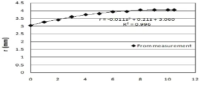
= 0.011 + 0.2 + 3.06 (45)

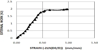
The neck profile obtained from image processing and Equation (45) are compared in Figure 6. As the figure suggests, Equation (45) accurately represents the neck profile. Therefore, this equation can be used with confidence for application of energy method. The volume of neck area calculated using Equation (45) and the experimental profile using image processing are compared in Table 2. As it is seen, the difference is so small and negligible. Variation of external work versus displacement and the external energy versus strain are depicted in Figures 7 and 8, respectively.

Figure 6. Comparison between the neck profiles from image

processing and Equation (45)

0 500 1000 1500 2000 2500

0 0.2 0.4 0.6 0.8 1 1.2

STR

ESS

(M

Pa)

STRAIN (mm/mm)

Figure 7. Variation of external work versus displacement

Figure 8. Variation of external energy versus strain

TABLE 2. Comparison between the measured and the

computed neck volumes

Initial volume of specimen (mm3_{) 4317.5}

The volume of uniform region after fracture (mm3_{) 3374}

The neck volume computed from the above two

measurements (mm3) 943.5

The neck volume computed from the proposed neck

profile (mm3) 912.34

Error in volumes % 3.3031

It is assumed that after the onset of necking, deformation accumulates only in neck area. In order to express Equation (40) in terms of the constant A and B, it must be integrated using a numerical method. The procedure of the method can be summarized as follows:

I. The strain at necking onset, εN, and its corresponding

stress are obtained from Figure 4. Substituting these parameters in Equation (41) we can write:

1363 = 0.46 + (46)

The energy density, , is measured from area under true stress-strain curve extending from origin up to the onset of necking. The strain energy due to uniform deformation is obtained from = . . The energy of uniform deformation for the test conducted in this work, is obtained 1.84 kJ and its density u = 426.4 MJ/ .This is the total strain energy of the total volume of specimen before necking.

II. The total external work from the beginning till fracture, is measured from load –displacement curve, or from Figure 7 as: ∫ . = 1986810 .

III. The constants of profile equation are determined as Equation 45.

In this method, for integrating Equation (40), neck region is divided to n=100 disks with equal length,∆ = 0.1. The region begins from = 0 and extends to

= = 10.45 . The coordinate z for each diskis calculated by =∆ + .After calculation of z, the radius of disk can be computed from Equation (45).

IV. Longitudinal strain, , for each disk is calculated as follows:

= , = =−2 (47)

where r is the average radius of the disk that is calculated in step ii and r0 is the initial radius of

specimen. It is to be mentioned that longitudinal and effective strains are equal (see Equation (10)).The computed equivalent strain is then substituted in Equation (40). After substituting the computed parameters, εN and u (from step i), (from stepiv), r

(from step iii) and the external work (from step ii) into Equation (40) and integrating, the equation reduces to:

40.378 + 113.853 = 145828(48)

V. Equations (46) and (48) are solved to give the values of the constants A and B:

A= 779.617 and B=1004.378.

5. VALIDATION OF ENERGY METHOD

The constants A and B are determined using several approaches. Optimization aided numerical simulation, Bridgeman-Leroy method and Bridgeman, Davidenkov and Siebel approaches are used for validation of energy method.

5. 1. Numerical Simulations Numerical simulation is used for validation of energy method. For this, the constants A and B are computed through simulation of tensile test and necking. In this approach, A and B are determined in a way that the experimental and numerical profiles of neck coincide. In order to do this, Genetic algorithm is employed to minimize the difference between the two profiles. Numerical simulations are performed using Abaqus software. Because of symmetry, only ¼ of the specimen is modeled. The model consists of 840 elements of the type CAX4R. This number of elements corresponds to the convergence of the results. The numerical model, its boundary conditions and a typical deformation after necking are shown in Figure 9. The lower surface of the specimen (z=0) is constrained against movement in z-direction( = 0). The specimen is loaded by applying a displacement of = 155 in z direction which simulates exactly the position control loading in the tensile tests. An objective function is defined as follows [18]:

OBJ(x, y) = a + a x + a y + a xy + a x + a y +

a x y (49)

where, x and y denote the unknowns A and B, respectively. On the other hand, objective function is also defined by:

in which the subscripts e and n denote the experimental

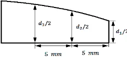
and numerical values of neck diameter. Three points on the neck are designated for the optimization process as shown in Figure 10. The points are located 5 mm apart with respect to the narrowest neck section. The experimental three neck diameters are measured through image processing technique. The numerical diameters are calculated for 7 different sets of A and B values as given in Table 3. The objective function is computed from Equation (50) and is substituted in Equation (49). The linear system of resulting seven equations is solved for the seven coefficients of Equation (50). The results are given in Table 4. The equation is then optimized using Genetic algorithm. The optimum values for A and B are obtained as A=807 and B=965.

Figure 9. The boundary conditions and a typical deformation

after necking

Figure 10. The designated points on the neck area for

optimization purpose

TABLE 3. Seven different sets of A and B and their

corresponding di’s

Item A B MODEING TEST

d1 d2 d3 d1 d2 d3 1 1045 864 6.98 7.4 7.6 6.1 6.6 8.1 2 870 938 4.8 7.34 8 6.1 6.6 8.1 3 1203 798 6.06 7.2 7.92 6.1 6.6 8.1 4 1100 841 7.52 7.8 8 6.1 6.6 8.1 5 905 923 4.97 7.32 8.08 6.1 6.6 8.1 6 607 1050 7.71 7.8 7.72 6.1 6.6 8.1 7 703.5 1009 7.75 7.96 8 6.1 6.6 8.1

TABLE 4. The constants of Equation 49

a7 a6 a5

a4 a3 a2

a1

0 -0.0798 0.0147

0 135.642 -32.535

-40413.38

Figure 11. The experimental and computed profiles of neck of

tested specimen

Figure 12. Variation of the ratio R/a versus time

5. 2. Bridgeman-Leroy Method In this method, the radius of neck curvature and the correction factor are obtained through the Equations (1) and (3). As: A=758

and B=1000.

5. 3. Bridgeman, Davidenkov and Siebel(B-D-S) Approaches In B-D-S models, the correction factor is a function of R/a in which R is the curvature radius of the neck. The neck profile is described by a second order polynomial. In this approach we can write:

= = (51)

The profile of the specimen exactly before fracture, tested in this work and the second order polynomial describing the profile are shown in Figure 11. Therefore, for Bridgeman method we have:

= = . = . = . (52)

Figure 13. Corrected stress-strain curves obtained using different techniques

TABLE 5. The values of strain energy and the external work

Item Energy (KJ)

External work 1.98681

Total strain energy of specimen

1.84098 before necking

Strain energy of neck region 0.14583 Total strain energy of specimen 1.98681

% Error -0.00016

TABLE 6. The values of A and B obtained using different

approaches and their errors respect to numerical method.

Energy Nume Bridg.- Bridg. David Sieb. Leroy

A (Mpa)

779.6 (3.4%) 807

758 (6%)

799 (0.8%)

755.6 (6.5%)

702.6 (13%) B

(Mpa)

1004.4 (4%) 965

1000 (3.6%)

995.4 (3.1%)

1015.3 (5.1%)

1039.6 (7.6%) Frac.

Stress (Mpa)

1784 (0.6%) 1772

1758 (0.8%)

1794.3 (1.2%)

1771 (0.1%)

1742.3 (1.7%)

The curvature radius is the same for all the three methods. The values of A and B for each method is provided in Table 5.

5. 4. External Work and Strain Energy The values of external work and the total strain energy corresponding to the neck and uniform areas of the deformed specimen are compared in Table 5. The total energy has been computed from energy method and the external work has been calculated from the load-displacement curve. As the table suggests the difference between the computed strain energy and the external work is absolutely small and quite negligible. This could be regarded as a benchmark for evaluating the accuracy of the method adopted in this investigation.

6. DISCUSSION

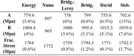
The values of A and B obtained using different approaches described in this work and their corresponding corrected stress-strain curves are provided in Table 6 and shown in Figure 13, respectively. It is hard to say which method gives the

best accuracy particularly when the results for the proposed method, Bridgeman and Bridgeman-Leory are very close. If we take the optimization method as a benchmark, it can be observed from Table 6 that best agreement is obtained for energy method and Bridgeman approach. We compared the differences of the quantities with respect to their corresponding numerical values given in the 3rd row of Table 6. The differences are given in parenthesis in the same table. The methods can now be compared more clearly with each other. The first interesting point is that the differences(except one case for Siebel) are well below 10%. As the results indicate and as far as A and B are concerned, Siebel gives the worst results and the proposed model and Birdgeman provide the best results, although differentiation between the proposed model and Bridgeman is difficult. We think that the dominant parameters in defining the corrected stress-strain curve are A and B and fracture strain is less important. The reason is that fracture strain is obtained from the fractured specimen. When the two parts of the broken specimens are put together to measure the neck section, the two parts usually don’t match exactly and therefore, the fractured neck diameter is always accompanied by some errors. As a result, we can conclude that the performances of the proposed model and Bridgeman model are close. It is a fact that all researchers have made some simplifications in their correction models. However, we may argue that optimization aided numerical simulations provide the most accurate prediction, because it provides the best agreement with the experiment for the neck profile. Having accepted this as the benchmark for assessing the accuracy of the models, we can see that the good agreement is obtained for the energy method discussed in this work.

7. CONCLUSIONS

8. REFERENCES

[1, 2] [3-17] [18] [19, 20]

1. Bridgman, P., "The stress distribution at the neck of a tension specimen", Transactions of the ASM, Vol. 32, (1944), 553-572. 2. Davidenkov, N. and Spiridonova, N., "Mechanical methods of testing-analysis of the state of stress in the neck of a tension test specimen", in Proceedings-American Society for Testing and Materials, Amer Soc Testing Materials 100 Barr Harbor Dr, W Conshohocken, Vol. 46., (1946), 1147-1158.

3. Siebel E. and Schwaigere S, "Mechanics of tensile test (in german)", Arch. Eisenhuttenwes, Vol. 19, (1948), 145-152. 4. Le Roy, G., Embury, J., Edwards, G. and Ashby, M., "A model

of ductile fracture based on the nucleation and growth of voids",

Acta Metallurgica, Vol. 29, No. 8, (1981), 1509-1522.

5. Needleman, A., "A numerical study of necking in circular cylindrical bar", Journal of the Mechanics and Physics of

Solids, Vol. 20, No. 2, (1972), 111-127.

6. Brünig, M., "Numerical analysis and modeling of large deformation and necking behavior of tensile specimens", Finite

Elements in Analysis and Design, Vol. 28, No. 4, (1998),

303-319.

7. Niordson, C.F. and Redanz, P., "Size-effects in plane strain sheet-necking", Journal of the Mechanics and Physics of

Solids, Vol. 52, No. 11, (2004), 2431-2454.

8. Fleck, N. and Hutchinson, J., "A reformulation of strain gradient plasticity", Journal of the Mechanics and Physics of Solids, Vol. 49, No. 10, (2001), 2245-2271.

9. Koc, P. and Stok, B., "Computer-aided identification of the yield curve of a sheet metal after onset of necking", Computational

Materials Science, Vol. 31, No. 1, (2004), 155-168.

10. Tang, C., Fan, J. and Lee, T., "Simulation of necking using a damage coupled finite element method", Journal of Materials

Processing Technology, Vol. 139, No. 1, (2003), 510-513.

11. Ling, Y., "Uniaxial true stress-strain after necking", AMP

Journal of Technology, Vol. 5, (1996), 37-48.

12. Mirone, G., "A new model for the elastoplastic characterization and the stress–strain determination on the necking section of a tensile specimen", International Journal of Solids and

Structures, Vol. 41, No. 13, (2004), 3545-3564.

13. Coppieters, S., Cooreman, S., Sol, H., Van Houtte, P. and Debruyne, D., "Identification of the post-necking hardening behaviour of sheet metal by comparison of the internal and external work in the necking zone", Journal of Materials

Processing Technology, Vol. 211, No. 3, (2011), 545-552.

14. Reddy, J.N., "Energy principles and variational methods in applied mechanics, John Wiley & Sons, (2002).

15. Cabezas, E.E. and Celentano, D.J., "Experimental and numerical analysis of the tensile test using sheet specimens", Finite

Elements in Analysis and Design, Vol. 40, No. 5, (2004),

555-575.

16. Yeh, H.-Y. and Cheng, J.-H., "Nde of metal damage: Ultrasonics with a damage mechanics model", International Journal of

Solids and Structures, Vol. 40, No. 26, (2003), 7285-7298.

17. Majzoobi, G., Freshteh-Saniee, F., Faraj Zadeh Khosroshahi, S. and Beik Mohammadloo, H., "Determination of materials parameters under dynamic loading. Part i: Experiments and simulations", Computational Materials Science, Vol. 49, No. 2, (2010), 192-200.

18. Majzoobi, G., Faraj Zadeh Khosroshahi, S. and Beik Mohammadloo, H., "Determination of materials parameters under dynamic loading: Part ii: Optimization", Computational

Materials Science, Vol. 49, No. 2, (2010), 201-208.

19. Gromada, M., Mishuris, G. and Ochsner, A., "Necking in the tensile test. Correction formulae and related error estimation",

Archives of Metallurgy and Materials, Vol. 52, No. 2, (2007),

231.

20. Standard, A., "E8," standard test methods for tension testing of metallic materials", Annual book of ASTM standards, Vol. 3, No., (2004), 57-72..

A New Technique based on Strain Energy for Correction of Stress-strain Curve

a _{Mechanical Engineering Department, Bu-Ali Sina University, Hamedan, Iran} b _{Islamic Azad University, Takestan Branch, Takestan, Iran}

P A P E R I N F O

Paper history:

Received 18 November 2013

Received in revised form 15 January 2014 Accepted in 06 March 2014

Keywords: Stress-strain curve, Correction factor Strain energy External work Numerical simulation هﺪﯿﮑﭼ

ﺶﻨﺗيﺎﻫﯽﻨﺤﻨﻣ

-يزﺎﺳﻪﯿﺒﺷردهﮋﯾوﻪﺑوداﻮﻣﮏﯿﻧﺎﮑﻣردﺶﻧﺮﮐ ﺪﻧرادرﻮﺧﺮﺑﯽﻧاواﺮﻓﺖﯿﻤﻫازاﺎﻫ

.

ﯽﻨﺤﻨﻣﻦﯾا زاًﺎﻣﻮﻤﻋﺎﻫ

ﯽﻣﺖﺳدﻪﺑﺶﺸﮐﺶﯾﺎﻣزآﻖﯾﺮﻃ ﯽﻣدوﺪﺤﻣنﺪﺷﯽﺋﻮﻠﮔهﺪﯾﺪﭘﺮﻃﺎﺧﻪﺑﻪﮐﺪﻨﯾآ

ﺪﻨﺷﺎﺑ

.

ﺶﻨﺗﯽﻨﺤﻨﻣ

-ﺎﺑﯽﺳﺪﻨﻬﻣﺶﻧﺮﮐ

اهدﺎﻔﺘﺳا هدﺎﺳرﺎﯿﺴﺑﻂﺑاورز ﺶﻨﺗﯽﻨﺤﻨﻣﻪﺑيا

-ﯽﻣﻞﯾﺪﺒﺗﯽﻘﯿﻘﺣﺶﻧﺮﮐ ﺪﻧدﺮﮔ

.

نﺪﺷﯽﺋﻮﻠﮔزﺎﻏآﻪﻄﻘﻧﺎﺗﻞﯾﺪﺒﺗﻦﯾا،ﺎﻣا

ﺖﺳاﺮﺒﺘﻌﻣ ، دادراﺮﻗﺮﻈﻧﺪﻣﻞﯾﺪﺒﺗﻦﯾارد ارﺶﻨﺗنﺪﺷيﺪﻌﺑ ﻪﺳﺪﯾﺎﺑﺪﻌﺑﻪﺑﻪﻄﻘﻧﻦﯾازااﺮﯾز

.

ﯽﻃ ﻪﻫد ﻪﺘﺷﺬﮔيﺎﻫ

شور ﯽﻨﺤﻨﻣﺢﯿﺤﺼﺗياﺮﺑﻦﻤﺠﯾﺮﺑشورﺪﻨﻧﺎﻣﯽﺋﺎﻫ ﺶﻨﺗيﺎﻫ -دﺎﻬﻨﺸﯿﭘﺶﻧﺮﮐ هﺪﺷ ﺪﻧا .

ﺮﺑﺪﯾﺪﺟشورﮏﯾ،ﻖﯿﻘﺤﺗﻦﯾارد

ﯽﻣﯽﻓﺮﻌﻣﯽﺸﻧﺮﮐيژﺮﻧا سﺎﺳا دﻮﺷ

.

هﺪﺷمﺎﺠﻧاﯽﺟرﺎﺧرﺎﮐﺮﺑاﺮﺑﯽﺸﻧﺮﮐيژﺮﻧاﻪﮐﺖﺳانآﺮﺑضﺮﻓ،شورﻦﯾارد

ﯽﻣ ﺪﺷﺎﺑ

.

شورﺎﺑﺪﯾﺪﺟشور ﻦﻤﺠﯾﺮﺑشورﺪﻨﻧﺎﻣﯽﻠﺒﻗهﺪﺷﻪﺋارايﺎﻫ

-ﻪﯿﺒﺷوﻞﺒﯿﯿﺳ،ﻮﮑﻧﺪﯾﻮﯾد،ﻦﻤﺠﯾﺮﺑ،يرﻮﺌﻟ ﻪﺑيزﺎﺳ

ﻪﻨﯿﻬﺑﮏﻤﮐ ﻪﺴﯾﺎﻘﻣيزﺎﺳ ﺖﺳاهﺪﺷ

.

ﺶﯿﭘﻪﮐدرادنآزاﺖﯾﺎﮑﺣهﺪﻣآﺖﺳدﻪﺑﺞﯾﺎﺘﻧ ﻪﺑﮏﯾدﺰﻧرﺎﯿﺴﺑيژﺮﻧاشورﯽﻨﯿﺑ

ﻪﯿﺒﺷشور ﻪﻨﯿﻬﺑﮏﻤﮐﻪﺑيزﺎﺳ ﯽﻣيزﺎﺳ

ﻪﻈﺣﻼﻣﻞﺑﺎﻗتوﺎﻔﺗ،لﺎﺣﻦﯿﻋردﺎﻣاﺪﺷﺎﺑ شورﺮﮕﯾدﺎﺑيا

ﻪﺴﯾﺎﻘﻣدرﻮﻣيﺎﻫ

دراﺪﻧ

.

ﻪﻧﻮﻤﻧياﺮﺑدﺮﺑرﺎﮐﻞﺑﺎﻗشورﻦﯾا يﺎﻫ

دﺮﮔوﺖﺨﺗ ، ﯽﻣود ﺮﻫ ﺪﺷﺎﺑ

.

doi: 10.5829/idosi.ije.2014.27.08b.15