A Fire Ignition Model and Its Application for Estimating Loss due to Damage of the Urban Gas Network in an Earthquake

Please cite this article as: A. Rajabipour, F. Behnamfar, A Fire Ignition Model and its Application for Estimating Loss due to Damage of the Urban Gas Network in an Earthquake, International Journal of Engineering (IJE), TRANSACTIONSB: Applications Vol. 29, No. 11, (November 2016) 1507-1519

International Journal of Engineering

A Fire Ignition Model and its Application for Estimating Loss due to Damage of the

Urban Gas Network in an Earthquake

A. Rajabipour, F. Behnamfar*

Department of Civil Engineering, Isfahan University of Technology, Esfahan, Iran

P A P E R I N F O

Paper history:

Received 02 April 2016

Received in revised form 30 September 2016 Accepted 30 September 2016

Keywords: Fire Ignition Model Loss Estimation Urban Gas Network Earthquake Damage

A B S T R A C T

Damage of the urban gas network due to an earthquake can cause much loss including fire-induced loss to infrastructure and loss due to interruption of gas service and repairing or replacing of network elements. In this paper, a new fire ignition model is proposed and applied to a conventional semi-probabilistic model for estimating various losses due to damage of an urban gas network in an earthquake with the aim of developing a reliable tool for better designation of resources. The suggested fire ignition model takes into account parameters such as density of gas, characteristics of gas dispersion in a city, distribution of power lines as sources of ignition, and wind speed. Because of several parameters involved, inevitably a logical combination of deterministic and probabilistic variables is applied in the loss estimation model. Economic impacts of spreading of fire, gas service suspension, and gas network damage are modeled within the same semi-probabilistic framework utilizing weight functions. Assessing different fire scenarios is possible in the model for loss estimation. The model is applied to selected examples of actual urban area earthquake scenarios and the results are discussed.

doi: 10.5829/idosi.ije.2016.29.11b.04

1. INTRODUCTION1

Earthquake loss estimates are forecasts of damage from future earthquakes and human and economic impacts that may arise [1]. As is asserted by FEMA [2], while loss estimation models are sophisticated, they are powerful tools for developing emergency plans and urban earthquake crisis management procedures [3, 4].

There are many studies in the field of loss estimation for buildings and lifelines. A general framework and formulation is proposed by the Pacific Earthquake Engineering Research Center (PEER) for probabilistic loss estimation. Using First Order Second Moment (FOSM) method, Baker and Connell have estimated the total uncertainty of the PEER formulation [5]. Brito and Almeida [6] developed a model for risk ranking of gas pipes using the multi-attribute utility theory. The model can be used by decision makers for prioritizing of critical sections of gas pipelines.

1_{*Corresponding Author’s Email: [email protected] (F. Behnamfar)}

gas release. The latter one needs models for ignition (developed herein) and fire spreading.

Fire following earthquake plays a remarkable role in the total loss due to an earthquake. For instance, based on a research done by San Francisco Department of Building Inspection, the fire following earthquake loss can reach $US 10.3 billion (2010) in this city. This loss is estimated to be in the range of $US 300-450 billion for Tokyo under 1923 earthquake in this city, based on a report by Risk Management Solutions [8]. In regard to loss of fire following an earthquake, gas-related damages account for 26% of fire ignitions where 56% is related to electrical damages and the rest has other causes [9]. The former source is considered in this paper.

At present the literature is under-developed regarding fire following earthquake, however significant researches have been launched in recent years. Models developed by Scawthorn have been frequently referenced in researches and technical reports in this area [10, 11]. His models consider building density, wind velocity and seismic intensity to estimate number of ignitions in an urban area. Trifunac et al. also developed empirical relations for estimating number of ignitions in urban area, considering data gathered from Northridge earthquake [12]. Moreover, HAZUS, as a well-known methodology for loss estimation, also uses empirical relations to calculate the expected number of ignitions [13]. Previous earthquakes data have been analyzed using generalized linear models with the aim of estimating location and number of ignitions due to an optional earthquake [14]. Ignitions stem from inside of structures have been estimated applying a probabilistic framework to analyze different events resulting in such ignitions by Zolfaghari et al. [15]. In contrast to the mentioned models that mostly have proposed empirical relations, an analytical approach is considered herein to develop the ignition model. This model is limited to ignition due to gas network damage and does not cover other sources of ignition.

American Lifeline Alliance (ALA) sets four design goals for a gas network. The goals are protecting public and social safety, maintaining system reliability, preventing monetary loss, and preventing environmental damage [16]. Regarding methods of measuring system performance, three general methods including graphic, localized and simulation methods are described in the above reference. In such a classification, this study uses the third method. Two approaches can be applied for seismic loss estimation including the deterministic and probabilistic methods. In the deterministic approach usually the amount of damage is measured by repair rate (repairs per unit of length or area) and the expected mean of damage is reported. Some equations for calculating repair ratio of buried pipes are presented in HAZUS [13]. Because of uncertainty existing in several parameters involved in the loss estimation process, the

deterministic approach cannot be solely applied in decision making for a city [1]. The proposed method in the present paper has a probabilistic framework, although some of the applied models are deterministic.

The main contribution of this study is developing a new ignition model for the fire of a gas network following an earthquake. Parameters such as density of gas, characteristics of gas dispersion in a city, distribution of power lines as sources of ignition, and wind speed are taken into account. Then the model is applied to a semi-probabilistic combination of various types of losses and the total loss is estimated as a function of elapsed time after occurrence of an earthquake. Three types of losses are considered including losses due to spreading of fire in urban areas (an induced physical loss), gas service disruption (a direct social economic loss), and damage of network elements consisting of pipes and regulators (a direct physical loss). Although it is possible also to estimate the indirect losses using the loss types considered in this study, no estimation will be given for this type of loss since the emphasis here is only on the physical losses.

2. THE BASIC MODELS

A model to estimate loss due to gas network fire needs models for pipe failure, spread of gas, ignition of fire, and fire spreading. These are called the basic models in this study. The general characteristics of the basic models are mentioned in Table 1. These models are described in more detail in the sections followed.

2. 1. The Probabilistic Model for Gas Pipe Failure

The gas pipe network includes two parts: the underground pipes, and the pipes attached to buildings. Failure of these two parts is considered separately.

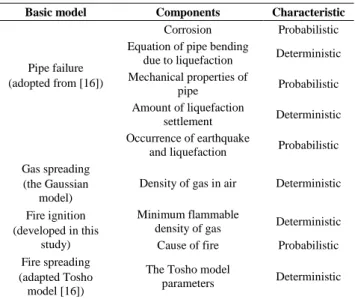
TABLE 1. General characteristics of the basic models

Characteristic Components

Basic model

Probabilistic Corrosion

Pipe failure (adopted from [16])

Deterministic Equation of pipe bending

due to liquefaction

Probabilistic Mechanical properties of

pipe

Deterministic Amount of liquefaction

settlement

Probabilistic Occurrence of earthquake

and liquefaction

Deterministic Density of gas in air

Gas spreading (the Gaussian

model)

Deterministic Minimum flammable

density of gas Fire ignition

(developed in this

study) Cause of fire Probabilistic

Deterministic The Tosho model

parameters Fire spreading

2. 1. 1. The Underground Gas Pipes The effect of earthquake on buried pipes can be divided into those due to wave propagation and those attributed to permanent ground deformations [17, 18]. It is perceived that pipe damage is mainly due to the latter effect in which about 80% of events appear as failure and the rest as leakage [19-22]. On the other hand, liquefaction is known to be responsible for about 88% of permanent ground deformation events in earthquakes [22]. Therefore, liquefaction is the main cause for pipe damage in potentially liquefiable areas. Numerous models have been developed for probabilistic estimation of pipe damage under earthquake. Much of these models predict number of failures in different parts of a network but some of them give the probability of failure of a certain pipe in a network. Since analysis of the network is a main step in developing the loss model, in the present study the behavior of each pipe of a network will be evaluated separately. Recently, the equally important phenomenon of corrosion has been considered when evaluating probability of seismic pipe damage. For the purpose of the present study the liquefaction-corrosion induced failure model proposed in the literature [16] was adopted as a more realistic approach. In this model, the bending angle of pipe is considered as the main parameter determining the pipe failure.

2. 1. 2. The Pipes Attached to Buildings Based on the observations and experimental research presented in the literature [23], pipes and regulators attached to a building are susceptible to failure when the building collapses. In addition, the mentioned report asserted that if the wall is not connected to a roof, court yard wall for instance, the attached pipe or regulator survives without major damage. In a certain part of a city, it is reasonable to assume that half of buildings have regulators attached to a roof-connected wall. Therefore, estimating the number of collapsed buildings in a certain earthquake in a city is essential.

Estimation of the number of the collapsed buildings can be accomplished using a damage index (DI). The DI represents the building performance against an earthquake and varies between zero and one. In this study, DI is estimated using the equation proposed by Bozorgnia and Bertero [24]. This is described as follows:

,

(1 )( )

1

e H

mon H mon

E DI

E

   _



   

_{ }



  (1)

in which:

e e

y

u u

  ₍₂₎

where α is a constant accepting values between 0 and 1 as a function of previous earthquakes, μ is displacement

ductility, ue is the maximum elastic displacement of a single degree of freedom system, uy is maximum displacement of the building under elastic condition,

μmon is monotonic displacement ductility capacity, EH is hysteretic energy demanded by the earthquake ground motion, and EH,mon is the hysteretic energy dissipation capacity under a monotonically increasing deformation.

The sources of uncertainty in building failure due to earthquake include uncertainty in structural behavior and uncertainty in seismic loading. In this research the structural behavior is evaluated deterministically by assuming the exact limit of DI=0.7 being equivalent to collapse [24]. For building evaluation, first an appropriate acceleration design spectrum is selected. Then the peak ground acceleration (PGA) required for each building type in the area to assume a value of DI=0.7 is determined using Equation (1). The probability of exceeding of PGA in the study area over the PGA corresponding to DI=0.7 is considered as the probability of failure of each building type. With the buildings' collapse probability and the number of buildings known, the total number of failures can be estimated. Therefore, in the process of estimating number of collapsed buildings, here the occurrence of earthquake is considered to be probabilistic while the structural behavior is assumed to be deterministic.

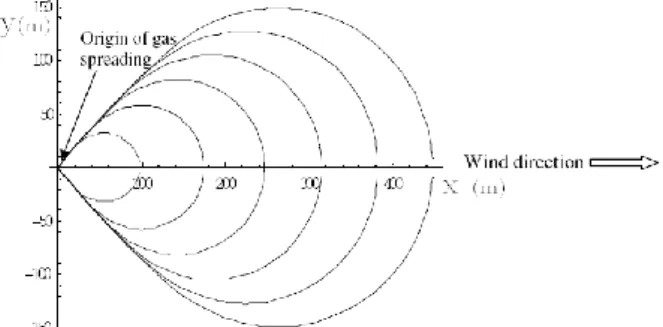
2. 2. Gas Spreading Model Several models have been proposed for gas spreading in air. These models cover sources like exhaust gas of a car, gas exiting from chimney of a factory, etc. For the gas spreading from an urban gas pipelines the Gaussian model is widespread. It is usually used for the gases having similar densities as air. In this model, the density distribution of gas is assumed to be bell shaped in the wind direction [25].

Figure 1 shows growing shape of a zone with a certain gas density using the Gaussian model. Similar distances between the contours in wind direction demonstrate the fact that growth rate of the plum can be assumed to be solely dependent on wind speed. Thus, it can be assumed that a certain density of gas spreads with almost a constant speed. This important result is used in the latter sections to estimate the time needed for ignition.

2. 3. The Proposed Model for Ignition of Gas

The basic idea for developing the fire ignition model in this study is the fact that adjacent excitations like sparks of power lines result in ignition of gas. This fire ignition model is developed for urban areas. In this regard, each excitation is taken as a trial having a certain probability of success. The other modeling assumptions are as follows:

 A certain density of gas is needed for ignition.  In densities more than the minimum density, the

 Similar characteristics are assumed for gas dispersion in a certain region of a city. These characteristics are: number of excitations in unit area (including power lines), wind speed and other parameters affecting gas dispersion.

Regardless of the source of excitation, the average number of excitations in a region in a time interval (t,t+Δt) can be estimated as:

( ) s t

nS t  t (3)

In which, S(t) denotes the area of flammable plume at time t; ρs isthe number of excitations in unit area; and ρt is the number of excitations in unit time. If time t is divided to m intervals, the probability of at least one successful trial (ignition) until a certain time t0(t0 is the moment in which ignition starts) is:

( ) .

1

0

( ) 1

,

M S t t m

s t

P m M k

t M

t



   



  

 





(4)

where, k denotes the probability of an unsuccessful trial (no ignition in a trial); and Δt is the elapsed time in each time interval. Because of constant characteristics in each region, k is constant. Therefore:

1 ( . )

( ) 1

M

m

S m t t

P m M k





 



   (5)

If the shape of gas plume is approximated with an ellipse, the area of flammable gas is estimated as:

2

( ) ( H* l)

S t V V t (6)

2

*

H l

V V V (7)

2 2

( ) ( . )

S t V m t (8)

Thus, the number of trials until time t is:

2 2

1 1

( . ) . ( . )

M M

m m

S m t  t  V m t t

 

    





t t

M

  (10)

Therefore, the probability of a successful trial (resulting in ignition) before time t is:

2 2 3

3 .

( ) 1

m V t

M

P m M k

 

 

 

 

 



   (11)

In which:

2 1

3

M m

m

M

_  (12)

Then the probability density function can be calculated as follows:

2_.3

( ) lim 1 V t M

F t k  



  (13)

2 1

3 2

(1 )(1 2 ) 1

lim lim lim

6 3

M m

M M

M

m _{M M}

M M

 

 



 _{ }

   (14)

Therefore: 2 _.3

3

2

( ) 1 V t

F t k

V

 

  

  

(15)

Derivation of f(t0) with regards to k gives: 3

3

( ) ln( )

t 2

f t k t k

 

  (16)

Figure 2 illustrates the probability density function (PDF) for ignition as a function of the elapsed time from the start of gas leakage.

Figure 1. Growing of gas boundary with a certain density

Figure 2.f (the probability density function ) as a function of

To calculate ν, the minimum flammable density of gas should be known. Experiments are needed to measure this parameter. As there is a linear relation between gas density in plume and discharge of the leaked gas, it can be assumed that in a certain region ν is proportional to gas discharge. Therefore, despite the need for tests, by knowing the pipe diameters and gas pressures in different regions it is possible to compare between different values of ν.

In the proposed formulation, k indicates the potential of a region for ignition. k is smaller in work times (9-17 hours) than in nights. In cold and wet nights k is a minimum and it is a maximum in hot and dry days.

2. 4. Models for Fire Spreading A comprehensive model for fire should cover two events, including ignition and spreading. The various existing models for fire spreading can be categorized as statistical, semi-computational, and computational methods. In the ignition model, estimation of number of ignition points is important. The Hamada model for fire spreading [26] has been used widespreadly. For example, HAZUS uses Hamada model as its fire spreading model [21]. A more precise model, the Tosho method, was proposed in 1997 and is used by Tokyo Fire Department [16]. An oval shape is presumed for the fire boundary in the Tosho model.

In the present study the Tosho model is used to estimate the rate of fire spreading but the spread direction is determined utilizing Equation (1). In the other words, the Tosho model is adapted here to take the urban open spaces into account. In this regard, growth of the burned boundary is supposed to be in the wind direction. Use of the vector of wind velocity in the fire spreading model helps modeling of obstacles like urban open spaces be easily accomplished. Thus, the vector of fire growth in unit time can be written as Equation (17).





( , , ) , ,

V x y U V x y n . U n (17)

where, U and U denote the vectors of wind blowing velocity and displacement, respectively; n is the boundary normal vector at the point (x, y) and V is the vector of fire growth in unit time.

3. THE LOSS ESTIMATION MODEL

The semi-probabilistic models described above for gas pipe failure, gas spreading and ignition, and fire spreading are now applied to the problem of estimating loss due to earthquake damage of an urban gas network.

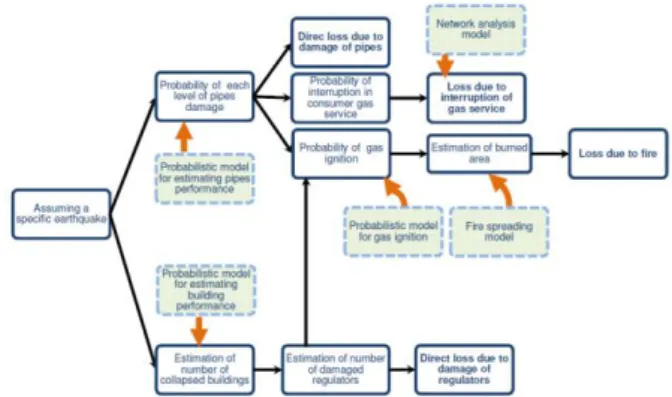
The diagram in Figure 3 schematically shows the suggested routine and its probabilistic components for estimating various losses due to damage of the urban gas network in a specific earthquake.

Figure 3. Proposed procedure for estimating loss

In this paper only physical losses directly related to gas network damage are considered. Thus, for example, loss due to building collapse as a direct result of an earthquake, not fire, is not modeled in the suggested method. Also indirect losses like injuries, death and psychological effects on humans are not figured out. Another important assumption is limiting the performance of the main pipes of each region only to feed (full pressure) and not feed (zero pressure) conditions, while in reality a range of different pressures in a pipe can be existing after an earthquake. In practice softwares specially developed for gas network analysis are used to estimate the working pressure at different nodes. With the help of an actual gas flow analysis, when the probability of seismic pipe failure is already calculated, the probability density function of gas pressure can be determined for the main pipe of each region. The exact analysis of gas network, that could have been done using a specialty software, was out of the scope of this research and was put aside for a later time. In the probabilistic model suggested in this work, the availability of the mentioned probability density function would result in a more accurate evaluation of the probability of feed and ignition of fire but that certainly would not alter the general aspects of the loss estimation model.

In the following sub-sections, components of the loss estimation model for calculating losses due to spread of fire in an urban area, interruption of gas service and damage of network elements, are described and then possible loss scenarios are discussed.

( ) ( ). . ( ).

F p Ig Ig F Ig Ig

l t p



In which, lF(t) is the average loss due to fire until time t;

pp is the probability of existence of flammable plume; fIg denotes the probability density function for gas ignition;

AF(t) denotes burned area until t, and tIg is the time of ignition.

3. 2. Interruption of Gas Service To emphasize the importance of this kind of loss, it should be mentioned that various industries including heavy sectors are consumers of gas service. For these consumers disruption of energy can cause a considerable amount of loss.

In this paper lss shows loss due to interruption of gas service. lss is a function of time, i.e., the more the time to reconnect gas service, the more the loss for consumers. Thus, lss not only depends on earthquake intensity but also on ability of technical teams to repair and return the gas system again to work.

In this study, the probability of interruption of gas service to a region has been calculated using the Fault Tree method. In this method gas network is modeled as nodes and connecting links. The set of links (pipes) with their malfunction causing interruption of gas flow in a region is called the Minimal Cut Set. Having the probability of pipes damage in an earthquake and the Minimal Cut Sets of a region, the probability of occurrence of a set of pipe damages causing cut-off in a region can be calculated. Details of the method are available elsewhere [28-30].

3. 3. Damage of Network Elements As experiences with previous earthquakes show, because of pipes being in huge numbers, these components are the most vulnerable elements in an urban gas network. This kind of loss can be divided into two types: damage of buried main pipes of each region, and damage of consumer pipes and/or regulators attached to buildings. This fact was explained in sections 2.1.1 and 2.2.2.

For the buried pipes, different probabilistic methods have been developed for estimating their performance subjected to earthquake [31]. HAZUS has suggested a probabilistic based formula for estimating number of damaged pipes for each level of damage [21]. The main ingredients of the HAZUS formula are peak ground velocity and displacement. In this study probability of underground pipe damage is calculated using the HAZUS procedure.

Regulators damage, as the main reason for fire in a gas network, is mostly due to collapse of the nearby building. Thus, to estimate the number of damaged regulators, the number of collapsed buildings must be estimated. Such estimation has normally to be applied to large areas with huge numbers of buildings. For this reason, the Damage Index (DI) has been used as an

effective tool to calculate the amount of earthquake damage in a building, as mentioned in section 2.2.2. Therefore, damage of regulators will need two prerequisites; first, regulator must be attached to a building (not to an independent wall), and second, building’s DI must be larger than a certain threshold, say, 0.7. If there is no information about regulators’ location, it can be assumed that half of regulators are attached to buildings and the other half to court walls across the street [23].

In this paper lMR is defined as the replacing cost of main pipes of a region, l1CD is the cost of finding, repairing/replacing damaged regulators as well as testing and making regulators ready to use and l2CD is cost of finding, repairing/replacing damaged consumer pipes plus testing and making consumer pipes ready to use.

As regulator damage depends on incidence of building collapse, the mean of l1CD is:

1CD i i 1CD n

l 



In which, n= Number of building types; mi= Number of building in type i; pi= Probability of collapse of a building in type i.

As it is assumed that in half of the buildings regulator is attached to a roof-connected wall, the number of collapsed buildings resulting in collapse of regulators will be 0.5



3. 4. Loss Scenarios and Mean of Loss To estimate each loss numerically and calculate its contribution to the total loss in a region, in this section possible scenarios and related assumptions for various losses are discussed.

3. 4. 1. Possible Events Immediately after an earthquake, for the main pipe of a region one of two conditions can be presumed: connected or interrupted. If the start or end nodes of a link (region main pipe) are being fed, the link is in connected condition. Then events I to IV and their sub-events in the order of criticalness may occur as follows:

I: Breakage of a region main pipe

 Gas service in the region is interrupted

 Main pipe of the region must be replaced

 Fire is probable in an area near the main pipe

 Consumer pipes and regulators may become damaged

II: Gas leakage from a region main pipe

 Main pipe of the region must be replaced; thus interruption in the region gas service will occur

 Fire is probable in an area near the main pipe

 Consumer pipes and regulators may become damaged

III: No damage in a region main pipe

 As consumer pipes are being fed, fire is probable due to damage of consumer pipes and/or regulators

 Consumer pipes and regulators may become damaged

IV: Disconnection of a region main pipe

 The gas service in the region is interrupted

 Region main pipe may break or leak

 Consumer pipes and regulators may become damaged

Based on the mentioned events, three forms of losses can be defined which are called lI, lII and lIII, noting

that fire is improbable in event IV.

3. 4. 2. Estimating Mean of Loss For loss estimation, the events and sub-events described in the previous section are utilized through their expected loss and probability of occurrence.

Parameters to be used are as follows: Re

( ) F

l t : Loss due to fire in a region when time t has elapsed

CD

l : Mean of loss in a region due to damage of consumers pipe and regulators

MR

l : Loss due to replacing main pipe of a region

SS

l : Loss due to interruption in gas service

( ) F i

l t : Fire loss in event i (i=I, II, III)

( ) j II

l t : Loss in event II when sub-event “j” has

happened (j=a, b, c defined in Figure 4) ( )

i

l t : Loss function in event i (i=I, II, III)

, ( )

Ig MR

f t : Probability density function for ignition due to main pipe’s break

, ( )

Ig CR

f t : Probability density function for ignition due to regulator’s break

, ( )

II I

f t : Probability density function for change of event

II to I

, ( )

II I

F t : Cumulative distribution function for change of event II to I

p

p : Probability of existence of the flammable volume of gas

n: Number of building types

i

m : Number of buildings in the ith type (1 ≤ i ≤ n)

i

p : Probability of collapse for buildings in the ith type

(1 ≤ i ≤ n)

j

p : Probability of occurrence of event j (j=I, II, III, IV) For simplicity, it is assumed that rate of fire spreading and value of burned assets are uniformly distributed in the region under study. Of course any other assumption is also possible and applicable in the model. Repair activities after an earthquake have not

been considered in the proposed model (see definition of lMR, l1CD, and l2CD in Sec. 3.3). In event I, fire can occur only adjacent to the main pipe of the region. Thus the expression related to fire loss inside the region vanishes in this event. If fire starts near the main pipe of a region at time tIg,

Re

( ) F Ig

l tt shows fire loss at time t.

Thus mean of loss in event I is:

( ) S F

I I I

l t l l (20)

In which:

S

I MR CD SS

l l l l (21)

Re , 0 ( ) ( ) ( ) Ig t F

I p _t Ig MR Ig F Ig Ig

l t p f t l t t dt





_

As defined previously, pp is the probability of existence of the flammable plum of gas. This parameter depends on weather conditions like wind speed and humidity [27].

In event II, one of the three sub-events is possible at time t. This fact is described in Figure 4. Therefore mean of loss in event II is:

, ,

( ) (1 ( )) ( ) ( ( )) ( ) (1 ) ( )

a b

II p II I II p II I II

c p II

l t p F t l t p F t l t

p l t

  

  (23)

In which:

Re , 0

( ) t ( ) ( )

a

II _T Ig CR F CD MR SS

l t f t l t T dT l l l





_



II I II p i i Ig CR II F II II

t

i F

I II II CD MR SS

l t

f t p p m f t l t t dt

l t t dt l l l

     _  _     _   







( )

c

II CD MR SS

l t l l l (26)

The parameters of the above formula are defined at the beginning of this section. In all sub-events of event II,

the loss includes lCD and lMR. Since interruption in gas service is also not avoidable, the term lSS also appears in loss formula in the three mentioned sub-events. If weather conditions are not suitable to form the flammable volume of gas, ignition will not be probable in event II.

Sub-event “c” refers to this situation. In sub-event “c” loss is solely limited to lCD , lMR and lSS. If fire occurs in event II, the region will switch to event I. Fire is probable inside the region because regulators are being fed, before fire is initiated at the main pipe. tII is

time of initiation of fire in the region; thus at time t, Re

F

l

would have time ttII to cause loss. When gathering of

the flammable volume of gas from the main pipe of a region is probable but no fire has been initiated from this pipe, region’s condition will be similar to event III. In this situation, regulators are being fed and fire is probable inside the region.

In event III consumer pipes and regulators will be damaged but main pipe of the region will not. In this event two types of losses including loss due to damage of consumer pipes and regulators and loss due to fire initiated from regulators are expected. Therefore regulators have the main role for the extent of loss in this case. The ith damaged regulator after time t causes

loss(t-Ti). Ti is the time between the regulator being

damaged and ignition of fire.

As noted earlier, failure of regulators is assumed to be solely because of building collapse. In this study the effect of failure of a building on failure of the adjacent building is neglected; therefore there is no cross-correlation in buildings collapse. With such an assumption, failures of regulators will also be independent of each other. Therefore, the total loss due to regulators damage is calculated as follows:





1

( ) ( )

n

III i i

i

l t E loss t T p m



 



The term loss(t-T) has two components as loss due to fire and loss due to damage of regulator itself. Therefore mean of loss in event III is as follows:

Re

1

( ) ( )

n

III F i i CD

i

l t E l t p m l 

 

 _{ }



Re Re

, 0

( ) t ( ) ( ) F p _T Ig CR F

E l t p f t l t T dT



   

 



In event IV no fire is probable neither from main pipe of the region nor from regulators. Thus mean of loss in this event is:

( ) ( ) ( ) IV SS I II MR CD

l t l t  p p l l (30)

Finally, based on the discussed events, mean of loss for a region when an earthquake occurs is as follows:

( ) ( )

[(1 )( ( ) ( ) ( ))]

IV IV

IV I I II II III III

L t p l t

p p l t p l t p l t



    (31)

In which:

pI, pII, pIII and pIV are probabilities of occurrence of events I to IV, respectively, calculated using the model described in Sec. 2.1 for pipe damage; L t( )is the mean

of total loss due to gas network damage for a region when an earthquake occurs.

Using Equation (31), it would be possible to calculate the proportion of each type of loss in the total loss.

Loss in a region includes lCD in all cases, which is related to the number of damaged regulators and consumer pipes. As mentioned previously, number of damaged regulators in a region can be estimated as 0.5



pipes can be estimated with Repair Rate defined in reference [22] as “repairs per 1000 feet or repairs per km”. Thus the share of lCD in Equation (31) is:

1 . 2

CD i i CD CD

Rl  l



In which:

RlCD: Share of lCD in the region’s total loss

R.R: Repair rate;

pl: Total length of pipes in the region;

lMR appears when computing loss for all events except event III. Using Equation (31) the proportion of

lMR in the total loss is:

( )

MR I II MR

Rl  p p l (33)

lSS appears in events I, II and IV. Its proportion in the total loss is:

[ (1 )( )]

SS IV IV I II SS

Rl  p  p p p l (34)

Loss due to fire depends on time; in fact the fire loss in each region is an increasing value with time (Equations (35-37)).

[(1 ) ] ( )

F F

I IV I I

Rl  p p l t (35)

[(1 ) ] ( )

F F

II IV II II

Rl  p p l t (36)

[(1 ) ] ( )

F F

III IV III III

Rl  p p l t (37)

There are a few suggested equations for fire spread rate. In this paper, fire spread rate is evaluated by the Tosho method [16]. In this method more parameters are considered in comparison with the previous methods like Hamada method which is used in HAZUS. The area of the burned zones is estimated with the method suggested in the literature [23]. In this method the direction of fire spreading is determined considering wind direction and the form of the fire boundary in each time step.

4. EXAMPLE OF APPLICATION

growth of loss functions is calculated. This in turn results in the ability to compare various types of losses in different regions and to compute the total loss.

4. 1. Basic Data As shown in Figure 5, the example network has 13 regions. Each region is defined as the area being fed from a certain main pipe. Dashed lines in Figure 5 show regions attributed to each main pipe. Each region is named using start and end node numbers. For example in region 1-2 start node of the main pipe is 1 and end node is 2. A number of properties are assumed to be identical in all regions; they are: probability of occurrence of the flammable volume of gas (pp), wind speed, and, humidity. pp is assumed to be 0.75 or example regions. It means weather condition is such that in 75 percent of days occurrence of the flammable volume of gas is probable.

Humidity and wind speed are supposed to be 35% and 3m/s, respectively. For earthquake scenario the design earthquake is considered, i.e., the earthquake with occurrence time of 475 years. As this is the standard earthquake of any seismic design code, for numerical analysis the design spectral values corresponding to the fundamental periods of the buildings are used. For calculating the fire loss, it is assumed that there is a linear relation between the amount of loss and the amount of burned area in a region. This is equivalent to assume a uniform distribution of assets in a region. Moreover, the regions are divided into two groups differing only in the fire spreading properties. Group A consists of the regions 3-6, 4-5, 5-7, 6-7, 6-9, 7-8, and 8-9, and Group B includes the regions 1-2, 1-3, 1-4, 2-5, 2-8, and 3-4. Properties of the regions are as follows.

a) Gas ignition

Gas ignition characteristics for use in the model developed in this study, Sec. 2.3, are presented in Table 2.

b) Fire spreading

Fire spreading properties corresponding to the Tosho method are given in Table 3.

In Table 3:

a: Plan dimension of the building,

d: Spacing between buildings (door to door),

b’: Ratio of non-damaged fire resistant structures to the total number of structures,

c’: Ratio of fire resistant structures,

νm: Fire speed inside fire resistant buildings,

νc: Fire speed inside collapsed buildings,

νnn: Fire speed from non-collapsed to non-collapsed buildings,

νnc: Fire speed from non-collapsed to collapsed buildings,

ν

νcc: Fire speed from collapsed to collapsed buildings.

c) Building types

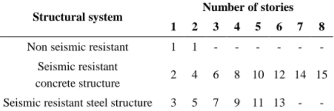
A type number is assigned to buildings with each structural system as presented in Table 4.

The buildings with the structural systems introduced in Table 4 are assumed to be distributed at identical percentages in all regions, as given in Table 5. Moreover, the collapse probability of each building type is calculated using the method described in Sec. 2.1.2 and presented in Table 5.

Using the method presented in Sec. 3.3, number of collapsed buildings will be 0.29N, where N is the total number of buildings.

Figure 5. Example network and its regions

TABLE 2. Gas ignition characteristics

Parameters of the probability density function ν (m2_/min2₎

k

Breakage of main pipes 0.0036 0.999

Leakage of main pipes 0.0018 0.999

Regulators 0.0018 0.999

TABLE 3. Values of the parameters of the fire spreading model (units: m. & sec.)

Parameters a d b' _c' _b

w fb νm νc νnnνnc νcc

Group A 12 2 Var. 0.8 10 4 25 30 24 24 20

Group B 30% of regions 12 2 Var. 0.8 10 4 33 35 31 31 22

70% of regions 15 19 15 15 12

TABLE 4. Type number of buildings with each structural system

Number of stories Structural system

8 7 6 5 4 3 2 1

- - - - - - 1 1 Non seismic resistant

15 14 12 10 8 6 4 2 Seismic resistant

concrete structure

TABLE 5. Percentage and collapse probability of each building type

Type of building 1 2 3 4 5 6 7 8 9 10 11 12 13 14 15 Percentage in

every region 8 5 4 15 12 18 10 9 7 4 2 3 1 1 1 Probability of

collapse (%) 100 4 15 46 75 49 61 54 75 63 77 80 73 69 70

4. 2. Probabilities of Pipe Events Regarding pipe events mentioned in Sec. 3.4.1, corrosion rate and liquefaction effects are considered and probabilities of break and leakage of pipes are calculated using the method presented in reference [16].

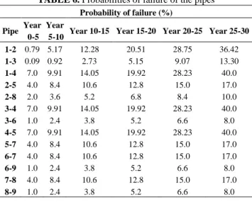
In this method the fragility curves of buried pipes are calculated considering corrosion rate, pipe diameter, soil properties and the site’s seismic risk. In this example it is assumed that these probabilities are known. Pipe diameters are given in Figure 6 and probability of pipes failure in Table 6.

Now, the probability of a pipe being fed or not can be calculated using the fault tree method. For instance, the probabilities of selected regions not being fed are presented in Figure 7. Using Table 6 and data similar to Figure 7, probabilities of events I to IV of Sec. 3.4.1 can be calculated.

4. 3. Estimating Losses in Each Region Among losses defined in Sec. 3.4.2, l1CD and lMR can be estimated using equations suggested by ALA [22]. In this example it is arbitrarily assumed that pipe damage in regions 1-2, 1-3, 1-4, and 3-4 is due to the permanent ground displacement and in other regions due to the earthquake wave propagation. With the number of collapsed buildings estimated as in Table 5, l_1CD can be calculated using Equation (19). On the other hand, in this example lSS is not estimated and just its proportion in the total loss is presumed to be a constant.

Figure 6. Diameters of pipes in the example network

TABLE 6. Probabilities of failure of the pipes

Probability of failure (%)

Pipe Year 0-5

Year

5-10 Year 10-15 Year 15-20 Year 20-25 Year 25-30

1-2 0.79 5.17 12.28 20.51 28.75 36.42

1-3 0.09 0.92 2.73 5.15 9.07 13.30

1-4 7.0 9.91 14.05 19.92 28.23 40.0

2-5 4.0 8.4 10.6 12.8 15.0 17.0

2-8 2.0 3.6 5.2 6.8 8.4 10.0

3-4 7.0 9.91 14.05 19.92 28.23 40.0

3-6 1.0 2.4 3.8 5.2 6.6 8.0

4-5 7.0 9.91 14.05 19.92 28.23 40.0

5-7 4.0 8.4 10.6 12.8 15.0 17.0

6-7 4.0 8.4 10.6 12.8 15.0 17.0

6-9 1.0 2.4 3.8 5.2 6.6 8.0

7-8 4.0 8.4 10.6 12.8 15.0 17.0

8-9 1.0 2.4 3.8 5.2 6.6 8.0

Figure 8. Fire loss for Group A regions under sub-event “a” of event II (see Figure 4)

To calculate the fire losses, using the Tosho method [16] a time-dependent function to estimate burned zones is obtained. As in this example a linear relation between the area of burned zones and the fire loss is assumed, the fire loss in each event can be estimated using the equations of Sec. 3.4.2. For instance, Figure 8 illustrates fire loss for Group A regions when the sub-event “a” of the event II, defined in Figure 4, occurs.

4. 4. The Total Loss To evaluate the proportions of various losses mentioned in Sec. 3, the total loss in a region is written as follows:

1 2 ( )

( ) ( )

( )

i i CD CD MR

F F

SS I II

F III

l t p m l a l b l

c l d V al l t e V al l t

f V al l t

                



(38)

In Equation (38), coefficients a to f show proportion of each loss at time t in a region and Val is value of assets per unit area of the burned zone. The coefficients can be calculated using Equations (32) to (37). For instance, Table 7 presents the coefficients calculated for the region 1-2 for a 30 year interval. In this table, area of the region is 72.6 ha, length of the 4” main pipe is 11,118 m, number of families in the first year is 430, and number of buildings in the first year is 134.

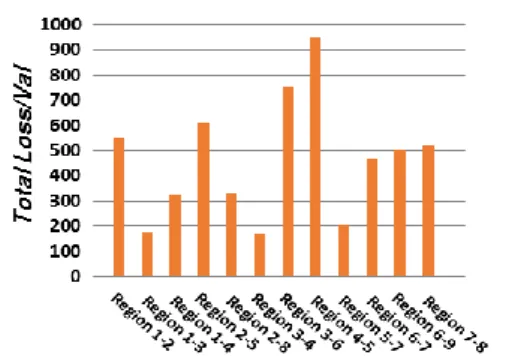
In Table 7 it can be concluded that because of liquefaction, the proportion of loss due to pipe damage is relatively large for region 1-2. Similarly, the loss due to gas service disruption is also considerable. Figure 9 illustrates mean of the fire loss 60 minutes after earthquake for a 30 year period. This figure can be used to compare between various regions regarding fire loss.

As seen in Figure 10, the fire loss is negligible in the early minutes after earthquake but it follows a linear and then a parabolic pattern afterwards. Figures like Figure 10 can be helpful for preparing a dispatching plan for fire fighters beforehand.

It can be concluded from Figure 10 that among all regions, region 4-5 is the most vulnerable region to fire and region 1-2 is the next one. In region 4-5 number of buildings is nearly 30 percent less than region 1-3.

Figure 9. Fire loss in different regions, 60 minutes after earthquake

TABLE 7. Coefficients a – f for the region 1-2 (see Equation (38))

Year of earthquake occurrence from the construction date

1-5 5-10 10-15 15-20 20-25 25-30

a 22 26 30 33 37 41

b 0.01 0.06 0.15 0.26 0.36 0.46

c 0.01 0.065 0.153 0.256 0.359 0.455

d 0.008 0.052 0.123 0.205 0.288 0.364

e 0.002 0.013 0.031 0.051 0.072 0.091

f 0.99 0.935 0.847 0.744 0.641 0.545

However, the larger probability of damage of the main pipe in region 4-5 and this region being in Group A, have caused the amount of fire loss in region 4-5 being more than 60% larger than 1-2 after one hour.

The obtained charts show estimation of various losses in each region in detail, allowing comparison between different regions. In addition, prioritizing and scheduling of emergency actions after an earthquake can be accomplished using these charts. Also, effective remedies for reducing amount of loss in each region may be developed by studying relations between network characteristics and losses. These characteristics include shape of the network, rate of degradation of pipe strength and size, building properties, weather condition, etc.

As is more evident with the above example, in the loss estimation model used in this study, the effects of corrosion, liquefaction, building collapse, gas leakage, and fire ignition and spreading are properly taken into account. Among the mentioned parameters, corrosion is a factor resulting in an increased level of loss through increasing the probability of pipe failure. The probability of failure in the pipes subjected to corrosion is a continuously increasing quantity with time. Therefore the model proposed here can trace the growth of different loss probabilities in each region and relate them to the corrosion rate. Using this information, a network repair policy can be devised and prioritized. On the other hand, type and arrangement of buildings in a city affect not only the failure level of regulators but also the gas dispersion and rate of fire spreading. The presented analysis can be useful in designing an appropriate urban planning scheme to minimize probable fire losses due to earthquake. Such a scheme can include criteria for minimum open spaces or mean of building to building distances.

5. CONCLUSIONS

A fire ignition model was developed and applied to the problem of loss estimation due to damage of the urban gas network in earthquakes in this study. The proposed model takes into account essential factors including density of gas, characteristics of gas dispersion in a city, distribution of power lines as sources of ignition, and wind speed. In the loss estimation procedure, the probable events instantly after an earthquake in regions of city are closely considered.

The loss estimation model evaluated in this study needs some basic models including a probabilistic model of pipe damage due to an earthquake, a model for initiating gas ignition and a fire spreading model. The advantage of the developed fire ignition model in comparison to the other models is its benefit from more physical parameters. This helped this study achieve a comprehensive formulation for loss and combine

various losses in a semi-probabilistic framework which cover all probable scenarios.

The loss diagrams calculated for each region in the example network illustrate how losses increase with time. A comparison between regions regarding each loss is also possible. Results of similar studies using the proposed semi-probabilistic model can help decision makers choose effective and efficient ways for reducing amount of loss in each region. Moreover, these results can be used to plan urban emergency activities after an earthquake. Further development of this model to enhance its accuracy and applicability seems to be necessary. This can include tasks such as accomplishing gas flow analysis within the model using the relevant specialty softwares as a part of loss estimation process, and developing a model for repair and maintenance of gas network after an earthquake.

6. REFERENCES

1. Ergonul, S., "A probabilistic approach for earthquake loss estimation", Structural Safety, Vol. 27, No. 4, (2005), 309-321.

2. Federal Emergency Management Agency (FEMA), “Assessment

of the state-of-the-art earthquake loss estimation

methodologies”, FEMA 249, Washington DC, USA, (1994). 3. Bendimerad, F., "Loss estimation: A powerful tool for risk

assessment and mitigation", Soil Dynamics and Earthquake Engineering, Vol. 21, No. 5, (2001), 467-472.

4. Taherinejad, M., Hosseinalipoor, S. and Madoliat, R., "Steady flow analysis and modeling of the gas distribution network using the electrical analogy (research note)", International Journal of Engineering-Transactions B: Applications, Vol. 27, No. 8, (2014), 1269-1276.

5. Baker, J. W. and Cornell, C. A., "Uncertainty specification and propagation for loss estimation using fosm method, Pacific

Earthquake Engineering Research Center, College of

Engineering, University of California, (2003).

6. Brito, A. J. and de Almeida, A. T., "Multi-attribute risk assessment for risk ranking of natural gas pipelines", Reliability Engineering & System Safety, Vol. 94, No. 2, (2009), 187-198. 7. Menoni, S., Pergalani, F., Boni, M. and Petrini, V., "Lifelines earthquake vulnerability assessment: A systemic approach", Soil Dynamics and Earthquake Engineering, Vol. 22, No. 9, (2002), 1199-1208.

8. Group, W. L., "Fire following earthquake: Identifying key issues for new zealand", Wellington Lifelines Group, Wellington, New Zealand, (2002).

9. Scawthorn, C., "Analysis of fire following earthquake potential for san francisco, california", SPA Risk LLC, for the Applied Technology Council on behalf of the Department of Building Inspection, City and County of San Francisco, (2010). 10. Scawthorn, C., "Simulation modeling of fire following

earthquake", in Proc. Third US National Conference on Earthquake Engineering, Charleston, August, (1986).

11. Scawthorn, C., Yamada, Y. and Iemura, H., "A model for urban post‐earthquake fire hazard", Disasters, Vol. 5, No. 2, (1981), 125-132.

13. Federal Emergency Management Agency (FEMA), “HAZUS MR4 Technical Manual”, Washington D.C, USA, (2003). 14. Davidson, R. A., "Modeling postearthquake fire ignitions using

generalized linear (mixed) models", Journal of Infrastructure Systems, Vol. 15, No. 4, (2009), 351-360.

15. Zolfaghari, M., Peyghaleh, E. and Nasirzadeh, G., "Fire following earthquake, intra-structure ignition modeling",

Journal of Fire Sciences, Vol. 27, No. 1, (2009), 45-79. 16. Tokyo Fire Department, Deterministic & measures on the causes

of new fire occurrence & properties of fine spreading based on an earthquake with a vertical shock, Fire Prevention Deliberation Council Report, (1997).

17. Mir Mohammad, S. and Moghaddas Tafreshi, S., "Soil-structure interaction of buried pipes under cyclic loading conditions",

International Journal of Engineering-Transactions B: Applications, Vol. 15, No. 2, (2001), 117-124.

18. Saberi, M., Behnamfar, F. and Vafaeian, M., "A continuum shell-beam finite element modeling of buried pipes with 90-degree elbow subjected to earthquake excitations", International Journal of Engineering-Transactions C: Aspects, Vol. 28, No. 3, (2014), 338-349.

19. Kobayashi, T., Shimamura, K., Oguchi, N., Ogawa, Y., Uchida, T., Kojima, S., Kitano, T. and Tamamoto, K., "Recommended practice for design of gas transmission pipelines in areas subject to liquefaction", in Workshop on Earthquake Resistant Design of Lifeline Facilities and Countermeasures Against Liquefaction, (2003).

20. Liu, X. and O'Rourke, M. J., "Behaviour of continuous pipeline subject to transverse pgd", Earthquake Engineering & Structural Dynamics, Vol. 26, No. 10, (1997), 989-1003.

21. Guideline for the design of buried steel pipe, ALA, (2002). 22. "Seismic fragility formulation for water systems, ALA, (2001). 23. Osaka Gas Company Japan, Center of Natural Disaster in

Industries Power and Water University of Technology (PWUT) Iran, Seismic Vulnerability Assessment, Rehabilitation and Crisis Management of the Great Tehran Gas Network, (2007). 24. Bozorgnia, Y. and Bertero, V. V., "Improved shaking and

damage parameters for post-earthquake applications", in Proceedings, SMIP01 seminar on utilization of strong-motion data, (2001), 1-22.

25. "ALOHA User manual, (March 2007).

26. Hamada, M., "On the rate of fire spread", Study of Disasters, Vol. 1, (1951).

27. Behnamfar, F. and Rajabipour, A., "Probabilistic estimation of fire spreading following an earthquake due to gas pipeline damage", in The 14th World Conference on Earthquake Engineering, (2008).

28. Aven, T., "Reliability and risk analysis", Springer Science & Business Media, (2012).

29. Blischke, W. R. and Murthy, D. P., "Reliability: Modeling, prediction, and optimization, John Wiley & Sons, Vol. 767, (2011).

30. Rajabipour, A., “Probabilistic assessment for enhancing seismic safety of buried pipes, case study on city gas system”, M.Sc. Thesis, Civil Eng. Dept., Isfahan University of Technology (IUT), Iran, (2007).

31. Toprak, S. and Taskin, F., "Estimation of earthquake damage to buried pipelines caused by ground shaking", Natural Hazards, Vol. 40, No. 1, (2007), 1-24.

A Fire Ignition Model and its Application for Estimating Loss due to Damage of the

Urban Gas Network in an Earthquake

A. Rajabipour, F. Behnamfar

Department of Civil Engineering, Isfahan University of Technology, Esfahan, Iran

P A P E R I N F O

Paper history:

Received 02 April 2016

Received in revised form 30 September 2016 Accepted 30 September 2016

Keywords: Fire Ignition Model Loss Estimation Urban Gas Network Earthquake Damage

ديكچ ه

یه ِلشلس کی رد یزْض ساگ ِکبض ِب ُذض دراٍ تاراسخ ىایس ذًاَت

صتآ سا یضاً تراسخ ِلوج سا یدایس یاّ ِکبض رد یسَس

کی ِلاقه يیا رد .ذضاب ِتضاد زب رد ار ،ِکبض یاضعا ضیَعت ٍ زیوعت ،یًاسر تاهذخ عطق سا یضاً تراسخ ٍ ،تخاس زیس صتآ لذه لذه .تسا ُذض داٌْطیپ یسَس تراسخ درٍآزب یازب مَسزه یتلااوتحا ِویً لذه کی رد یداٌْطیپ

فلتخه یاّ

صیصخت تْج داوتعا لباق راشبا کی ِعسَت راک يیا سا فذّ .تسا ُذض ُدزب راک ِب ،یزْض ساگ ِکبض ىذید بیسآ سا یضاً یه عباٌه زتْب صتآ لذه رد .ذضاب

تایصَصخ ،ساگ یلاگچ ىَچوّ یلهاَع زثا یداٌْطیپ یسَس عیسَت ،زْض رد ُذض زطتٌه ساگ

لذه رد ،نّ ِب ظبتزه لهاع يیذٌچ دَجٍ لیلد ِب .تسا ُذض ِتفزگ زظً رد ،داب تعزس ٍ ،لاعتضا عباٌه ىاٌَع ِب یلصا طَطخ تاهذخ عطق ،صتآ شزتسگ یداصتقا تازثا .تسا ُذض ُدزب راک ِب یٌیعت ٍ یتلااوتحا یاّزییغته سا یبیکزت تراسخ درٍآزب اسخ ٍ ،ساگ ُذض یساس ِیبض ،یًسٍ عباَت سا ُدافتسا اب ٍ ِباطه یتلااوتحا ِویً راتخاس اب لذه سا ُدافتسا اب شیً ،ساگ ِکبض ِب تر

صتآ فلتخه یاَّیراٌس یبایسرا .تسا ىاکها تراسخ درٍآزب لذه رد یسَس

یه زیذپ لاثه رد یداٌْطیپ لذه سا .ذضاب یاّ

َیراٌس سا یعقاٍ یزْض ِیحاً رد ِلشلس یاّ

.تسا ِتفزگ رازق یسرزب درَه ىآ جیاتً ٍ تسا ُذض ُدافتسا