Experimental Research of Statistical Characteristics
of Wind Wave Breaking
A. E. Korinenko
1,*, V. V. Malinovsky
1, V. N. Kudryavtsev
1,2 1Marine Hydrophysical Institute, Russian Academy of Sciences, Sevastopol, Russian Federation*e-mail: [email protected]
2Russian State Hydrometeorological University, Saint-Petersburg, Russian Federation The results of characteristics’ analysis of the wind wave breaking (length, velocity, direction) ob-tained in the Black Sea in September-October, 2015 from the oceanographic platform in Katsiveli are presented. Wave breaking was recorded by a video camera synchronously with the measurements of wind waves and meteorological parameters. The algorithm based on calculating the threshold deter-mined at analyzing the distribution function of the video signal brightness was applied to identify breaking using the video records. The optical equipment used in the experiment made it possible to reliably identify the breaking generated by the waves with the lengths greater than 4 m and the phase velocities exceeding 2.5 m/s. The data obtained correspond well to the model conceptions of O.M. Phillips which were developed for the equilibrium interval of the wind wave spectrum. The histograms of the wave breaking velocities at the wind speeds 10–16 m/s are given. It is shown that at the developing waves, the breaking waves’ phase velocity can reach that of the wind waves corre-sponding to the spectral peak, while at the developed waves, no breaks with the velocities exceeding a halfphase one of the waves corresponding to the spectral peak were observed. Probability densities of the breaking lengths in the wind speeds’ measured range are described by the power law with the exponent -3.23. Distribution of the breaking orientations is described well by a degree of the angle cosine, at that the exponent decreases linearly from 5 to 4 with the wind speed increase from 10 to 16 m/s.
Keywords: wind wave breaking, in situ studies, wave breaking orientation, breaking lengths’ distri-bution, wind waves’ spectrum.
Acknowledgements: the investigation is carried out within the framework of the state task on the theme No. 0827-2018-0003 “Fundamental studies of the oceanological processes conditioning the marine environment state and evolution under the influence of natural and anthropogenic factors based on the observational and modeling methods”. V.N. Kudryavtsev points to financial support of the RSF grant No. 17-77-30019.
For citation: Korinenko, A.E., Malinovsky, V.V. and Kudryavtsev, V.N., 2018. Experimental Re-search of Statistical Characteristics of Wind Wave Breaking. Physical Oceanography, [e-journal] 25(6), pp. 489-500. doi:10.22449/1573-160X-2018-6-489-500
DOI: 10.22449/1573-160X-2018-6-489-500
© 2018, A. E. Korinenko, V. V. Malinovsky, V. N. Kudryavtsev © 2018, Physical Oceanography
Introduction
Wind wave breaking (WWB) plays an important role in the processes related to the gas exchange between the ocean and the atmosphere [1], wave energy dissipation [2], generation of turbulence in the near-surface sea layer [3].
The parameter used in different radiophysical tasks is the length of breaking crest Lb. In [6], a significant role of the drops generated by WWB when scattering
in the 8-millimeter range of electromagnetic waves is shown, and the intensity of the dropsis determined by Lb value. A model of nonresonant scattering component
(related to WWB) at small grazing angles on the horizontal polarization was proposed in [7], where it was shown that the normalysed radar cross section depends on Lb and thewave breaking orientation.
A number of studies on the WWB lengths and orientations have been per-formed to date. In one of the first works [8] devoted to the study of breaking statis-tical characteristics, the probability densities of Lb values, well described by the
gamma distribution, and the histograms of breaking orientations, described by the normal distribution, were obtained. The results of field experiment analysis are presented in [9], where Lb distribution is requested to be described by an
exponen-tial law. The histograms of breaking lengths and orientations are given in [10], and in [11] it is shown that at young waves the breaking rates can reach the phase ve-locity of the spectral peak waves, while at fully developed waves the ones of the spectrum equilibrium range break.
Breaking is the main source of wind-wave energy loss in the gravitational in-terval [2]. Therefore, the concepts of WWB angular distribution are required to validatethe existing models of wave energy dissipation.
Despite a great number of works devoted to the study of breaking statistical characteristics, their comparisons with the model calculations are practically ab-sent. The orientation of breaking lengths under various hydrometeorological condi-tions has not been sufficiently studied.
The purpose of this work is to analyze the statistical characteristics of wind-wave breaking obtained under field conditions, and to compare experimental de-pendencies with the existing models.
The methods of data processing and experimental conditions
Field experiments were carried out in September – October 2015 from a stationary oceanographic platform located in the Blue Bay near Katsiveli village (the Southern Coast of Crimea). The oceanographic platform is installed ~ 480 m from the nearest point of the coast and has 44º23ʹ38ʹʹ N, 33º59ʹ09ʹʹ E coordinates. In the area of the platform the depth is about 30 m.
In this work the determination of wind-wave breaking characteristics was car-ried out using video recordings of the sea surface made with a digital video camera located at 11.4 m height above sea level. The viewing direction was 30°–40° to the horizon, in the azimuthal plane – about 50°–60° to the “up-wind” direction. The use of a lens with 54° horizontal and 32° vertical viewing angle provided video recording of the region (area) on the sea surface in the form of a trapezium with 14–16 and 29–48 m base lengths. Video recording was carried out with 25 frames per second rate and 1920 × 1080 pixels resolution.
by zero. Subsequent data processing consisted in dividing the breaking process into two phases – the active crest and the passive foam. The selection of the active foamwas based on the differences in the kinematic characteristics of these phases [12]. Processing of videos was carried out automatically.
Further, the selected areas were divided into groups all points in which belong to areas related in space and time. As a result, a set of groups, each of which was information about the active phase evolution of the individual breaking, was ob-tained for all series of measurements.
In order to determine physical dimensions of breaking each video frame with a known observation geometry and camera parameters (tilt angle, matrix dimen-sions, focal length and lens viewing angles) was transformed into a rectangular sys-tem of horizontal coordinates on the sea surface. Depending on the angle of the video camera’s lens field of view, the maximum spatial resolution made up ~ 1 cm, the minimum one ~ 2.5 cm. As a result, the breaking area 𝑆𝑆𝑖𝑖𝑗𝑗, its maximum linear
𝑗𝑗
dimensions , which are the lengths of the major axes ellipses approximating the breaking region according to the method [12], were calculated for each group. Along with the above mentioned parameters, the coordinates of mass center posi-tion (𝑥𝑥𝑖𝑖𝑗𝑗,𝑦𝑦𝑖𝑖𝑗𝑗), where index 𝑖𝑖 is the number of breaking belonging to the group and 𝑗𝑗 is the number of a group were found. Average modulus of breaking motion
veloci-ty and propagation direction were calculated as follows: 𝑐𝑐𝑗𝑗 =�(𝑐𝑐𝑥𝑥𝑗𝑗)2+ (𝑐𝑐𝑦𝑦𝑗𝑗)2,
𝜙𝜙𝑗𝑗= arctan (𝑐𝑐
𝑦𝑦𝑗𝑗�𝑐𝑐𝑥𝑥𝑗𝑗), where 𝑐𝑐𝑥𝑥𝑗𝑗, 𝑐𝑐𝑦𝑦𝑗𝑗 are the velocity components which were
de-termined by the mass center motion using the method of the least-squares error method.
The result of processing is a database containing the information about linear dimensions of the breaking in time and space, average modulus of mass center mo-tion velocity of breaking crest and its direcmo-tion.
Meteorological information was collected by Davis 6152EU multifunctional complex located at 23 m height above the sea level on the mast of the oceano-graphic platform. The measured wind velocity was recalculated into effective neu-tral stratified wind velocity U at 10 m height according to the method [13].
Surface wave characteristics were recorded using a grid of 6 string wave re-corders located in the center and tops of a regular pentagon with 0.25 m circumra-dius. The distance of wave recorder grid to the nearest platform element exceeded 10 m.
As a result of wave recorder data processing, we used the maximum entropy method to calculate frequency-angular spectra of the sea surface elevations
𝑆𝑆(𝑓𝑓,𝜙𝜙), to determine the frequencies of wind waves spectral peak 𝑓𝑓𝑝𝑝, directions of general propagation of wind waves 𝜙𝜙𝑝𝑝 and swell waves, the significant wave heights 𝐻𝐻𝑠𝑠 (𝐻𝐻𝑠𝑠= 4√𝜎𝜎2, where 𝜎𝜎2 is the dispersion of sea surface elevations).
As is known, in natural conditions, in addition to the wind waves, there are swell waves the evolution of which is not described within the local energy balance characteristic of the equilibrium interval.
In order to divide the frequency spectrum of waves into swell waves and wind ones, we used the method proposed in [15], in which the measured spectrum of
𝑆𝑆(𝑓𝑓) waves was compared with the theoretical spectrum 𝐹𝐹(𝑓𝑓) [14]: 𝐹𝐹(𝑓𝑓) =
2𝜋𝜋𝜋𝜋𝑢𝑢∗𝑔𝑔(2𝜋𝜋𝑓𝑓)−4, where 𝜋𝜋= 0.06–0.11; 𝑢𝑢∗ is dynamic velocity; 𝑔𝑔 is the
gravita-tional acceleration. According to this method, the spectrum area which lies above the lower boundary (𝜋𝜋= 0.06) belongs to wind waves, and if the spectrum area is situated below the boundary, then the measured waves are classified as swell ones.
Our measurements were carried out within 10–16 m/s range of wind velocities. The main criterion for the measurement data selection was the stationarity of wind ve-locity and direction over several hours. For the analysis we selected the cases when the angle between the directions of swell waves and wind velocity did not exceed 30°.
General information on the experimental conditions is given in the table (measurement date; average wind velocity 𝑈𝑈� and its direction 𝜑𝜑𝑈𝑈�; 𝐻𝐻𝑠𝑠; wave age
𝛼𝛼=𝑐𝑐𝑝𝑝/𝑈𝑈, where 𝑐𝑐𝑝𝑝 is the phase velocity of the waves at the frequency of spectral
peak 𝑓𝑓𝑝𝑝).
Measuring conditions
Date urement seriesNo of meas- 𝑈𝑈�, m/s 𝜑𝜑𝑈𝑈�° 𝐻𝐻𝑠𝑠, m 𝛼𝛼 𝑓𝑓𝑝𝑝°
10.09.2015
1 11.8 85 1.1 0.6 0.21
2 11.7 85 1.1 0.6 0.21
3 10.9 85 1.2 0.8 0.19
11.09.2015
1 10.0 90 0.8 0.6 0.28
2 10.3 90 0.8 0.6 0.26
3 11.0 90 0.8 0.6 0.26
12.09.2015
1 14.6 70 1.2 0.4 0.28
2 16.1 75 1.2 0.3 0.29
3 15.2 85 1.4 0.4 0.25
08.10.2015
1 13.2 70 1.3 0.4 0.29
2 13.4 80 1.5 0.5 0.24
3 11.7 80 1.5 0.6 0.24
11.10.2015 1 13.6 70 2.2 0.8 0.14
12.10.2015 1 14.4 65 2.2 0.8 0.13
2 15.0 65 2.0 0.7 0.14
The results of field measurements
into account the dispersion relation, the estimation of probability of wind wave breaking of various lengths.
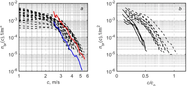
The distributions of breaking rates per surface unit 𝑛𝑛br(𝑐𝑐), obtained from each videotape, are shown in Fig. 1, a. In the presented data, at 𝑐𝑐>2.5–3 m/s a sharp drop in 𝑛𝑛br(𝑐𝑐) is observed with increasing breaking rates. When 𝑐𝑐<~ 2.5 m/s the slope of histograms is significantly smaller and in a number of records 𝑛𝑛br(𝑐𝑐) val-ues are almost constant in this interval. Such feature of the histograms of breaking characteristics is explained in detail in [16]. This is due to the fact that when using optical equipment a large number of breakings formed by short waves are not iden-tified during the video processing.
F i g. 1. Statistical characteristics of wave breaking rates: a – histograms of wave breaking velocities at the wind velocities 10–16 m/s (solid lines are the results of calculations by formula (9) (see p. 496) for the wind velocity 10 m/s (blue curve) and 16 m/s (red curve)); b – histograms of the relation of wave breakingrate to the phase velocity correspondingto the spectral peak in the wave age range 0.3–0.5 (dash line) and 0.65–0.8 (solid line)
Fig. 1, b shows 𝑛𝑛br(𝑐𝑐), where the values of 𝑐𝑐/𝑐𝑐𝑝𝑝 ratios characterizing the spectral interval of breaking wave are indicated on the abscissa axis. With develop-ing waves, the phase velocity of the breakdevelop-ing waves reaches the phase velocity of the wind waves of the spectral peak. With the development of waves, we did not observe breakings moving at the velocities above 0.5 𝑐𝑐𝑝𝑝. The obtained result corre-lates with the experimental data [11, 17].
Distribution of breaking lengths.We consider statistic characteristics of 𝐿𝐿b breaking lengths determined as the foam line size in the direction parallel to the crest of breaking wave. In Fig. 2 the points show the distribution 𝑝𝑝 (𝐿𝐿 b) obtained in each videotape at different hydrometeorological conditions. Despite a rather wide range of measurement conditions, all distributions are rather similar.
As follows from Fig. 2, a, the densities of breaking length probabilities are generally close to the power law
𝑝𝑝(𝐿𝐿b) =𝜇𝜇𝐿𝐿−𝜌𝜌b . (1)
F i g. 2. Statistical characteristics of the wave breaking lengths resulted from all the records: a – dis-tribution of Lbvalues; b – wind dependence of the wave breaking average length (circles), solid line denotes data approximation by linear dependence
b m
b m
b m
From Fig. 2, b it follows that with 𝑈𝑈 increase from 10 to 16 m/s average val-ues of 𝐿𝐿 increase from ~0.7 to ~0.9 m. Straight line shows linear dependence 𝐿𝐿
= 0.47 + 0.027𝑈𝑈 the inclination of which is close to 0.034 value obtained in [8]. Weak wind dependence of 𝐿𝐿 values can be explained by sharp decrease of
𝑝𝑝(𝐿𝐿b) with the growth of WWB length. Indeed, the average length of the breaking
major axis is equal to the first moment of random variable Lb. Then, taking into
account (1) and the obtained inclination ρ, we can estimate 𝐿𝐿bm~�Lminb �−2.23−
(Lbmax)−2.23, where Lbmin and bmaxare the minimum and the maximum values of
registered Lb. Thus, 𝐿𝐿mb is mainly determined by its minimum size Lminb (specified when analyzing the data) and increases with 𝐿𝐿maxb growth and increase of the wind.
Distribution of breaking orientation. In Fig. 3 the example of angular distri-bution histograms of breaking number obtained on September 10 and 12, 2015 dur-ing the second series of measurements, is shown. Solid line indicates the approxi-mation by the function
𝑃𝑃𝑛𝑛(𝜙𝜙) =𝐴𝐴cos𝑝𝑝(𝜙𝜙). (2)
For convenience of comparison, all angular distributions were normalized as
𝑛𝑛br(𝜙𝜙) is a number of breakings in the direction 𝜙𝜙. The origin of coordinates
cor-responds to the maximum of distribution. It can be seen that the distributions of orientations have symmetric unimodal form and are well described by the expres-sion (2).
The dependence of 𝑝𝑝 values (obtained for all data) on wind velocity is shown in Fig. 4, a where rather significant scattering of points is observed. Nevertheless, a weak wind dependence of the exponent is observed, which can be approximated by a linear function p = 6.5–0.15U (solid line). The p values obtained at various wave ages are shown in Fig. 4, b, where the absence of an explicit dependence of the exponent on α is obvious.
F i g. 4. Dependence of exponent 𝑝𝑝 (formula (2)) on the wind velocity– a and wave age – b
Discussion of the results
The breakings visualize energy dissipation of wind waves. It is believed that breaking is the main mechanism responsible for the discharge of gravitational waves energy in the equilibrium range of the spectrum. The distribution of breaking waves by the direction of motion is an important characteristic that allows us to relate spatial characteristics of breaking to the angular spectrum of the surface waves.
In order to assess the statistical characteristics of wind-wave breaking, we use the breaking statistics proposed by O. M. Phillips [14]: the author describes dynam-ic, kinematic and statistical properties of the WWB through the length of the crest of the breaking wave moving at
c
velocity. Λ(𝐜𝐜)-function w as p roposed – t he d is-tribution of the total length of breaking crests per surface unit within the range of velocities (с, с+dc). Theintegral ∫ Λ(𝐜) dc is the total length of thebreakingcrests per unit of the sea surface area.Assuming that the WWB are geometrically similar, the average length of breaking crests will be proportional to𝑘𝑘 −1, where k is a wave number of breaking wave. Then the number of 𝑛𝑛br breakings per unit of the area will be proportional to:
𝑛𝑛br ~ 𝑘𝑘Λ(k)𝑑𝑑𝐤𝐤, (3)
𝜋𝜋⁄2
−𝜋𝜋⁄2 −𝜋𝜋⁄2𝜋𝜋⁄2
where Λ(k)is total length of breaking crests per surface unit within the range of wave numbers (𝐤𝐤 , 𝐤𝐤 + 𝑑𝐤). It should bepointed out that in the transition from
Λ(𝐜𝐜 ) to Λ(k) the dispersion relation for gravitational waves in deep water 𝜔𝜔 2
= and the expression for phase velocity 𝑐𝑐 2 = 𝑔𝑔 ⁄𝑘𝑘 are used.
An important conclusion of O. M. Phillips theory is the connection of Λ-function with the average rate of energy dissipation 𝐷𝐷(k) on the unit of surface due to breakings [14]:
𝐷𝐷(k) =𝑏𝑏𝑔𝑔3 2⁄ 𝑘𝑘−5 2⁄ Λ(k), (4) where 𝑏𝑏= 0.03–0.07 is dimensionless parameter [18].
In order to find 𝐷𝐷(k) we consider the energy balance in equilibrium interval of surface wave spectrum. According to [14], energy dissipation due to breakings will be proportional to the energy input from the wind:
𝐷𝐷(k) = 𝑔𝑔𝜔𝜔𝑔𝑔(𝑘𝑘,𝜙𝜙)𝐹𝐹(k), (5)
where 𝑔𝑔(𝑘𝑘,𝜙𝜙) is a coefficient of wind-wave interaction; 𝐹𝐹(k) is a spectrum of ele-vations.
From (4) and (5) we can obtain the expression Λ(k) =𝑏𝑏−1𝑘𝑘3𝑔𝑔(𝑘𝑘,𝜙𝜙)𝐹𝐹(k), substituting which in (3) we write down 𝑛𝑛br in the following form:
𝑛𝑛br(𝐤𝐤)~𝑏𝑏−1𝑔𝑔(𝑘𝑘,𝜙𝜙)𝑘𝑘4𝐹𝐹(k). (6)
In [19] an expression for wind-wave interaction 𝑔𝑔(𝑘𝑘,𝜙𝜙) =𝐶𝐶𝛽𝛽(𝑢𝑢∗⁄𝑐𝑐)2cos2𝜙𝜙, where 𝐶𝐶𝛽𝛽 is a parameter, is proposed. In the variables (𝜔𝜔,𝜙𝜙), taking into account the dispersion relation, the expression (6) can be written as
𝑛𝑛br(𝜔𝜔,𝜙𝜙)~𝑏𝑏−1𝐶𝐶𝛽𝛽𝑢𝑢∗2𝑔𝑔−6cos2𝜙𝜙 𝜔𝜔10𝑆𝑆(𝜔𝜔,𝜙𝜙). (7)
According to (7), the azimuthal distribution of number of breakings generated by the waves from frequency interval (𝜔𝜔0,𝜔𝜔1) will be written as
𝑛𝑛br(𝜙𝜙)~𝑏𝑏−1𝐶𝐶
𝛽𝛽𝑢𝑢∗2𝑔𝑔−6∫𝜔𝜔𝜔𝜔01cos2𝜙𝜙 𝜔𝜔10𝑆𝑆(𝜔𝜔,𝜙𝜙)𝑑𝑑𝜔𝜔, (8)
where 𝜔𝜔0= 1.5𝜔𝜔𝑝𝑝 and 𝜔𝜔1 are the upper and the lower boundaries of equilibrium interval, respectively [20]. As it was mentioned above, the applied method provides a reliable recording of breakings the velocity of which exceeds 2.5 m/s. Then, for our conditions 𝜔𝜔1= 4 rad/s.
Expression (7) allows one to estimate the number of breakings on the surface unit within the range of velocities (с, с+ dc). Integrating (7) over the azimuth, tak-ing into account the dispersion relation in the variables c, we can write down
𝑛𝑛br(𝑐𝑐)~𝑏𝑏−1𝐶𝐶𝛽𝛽𝑢𝑢∗2𝑔𝑔2𝑐𝑐−7∫ cos2𝜙𝜙 𝐵𝐵(𝜔𝜔,𝜙𝜙)𝑑𝑑𝜙𝜙 𝜋𝜋
2
−𝜋𝜋2 , (9)
where 𝐵𝐵(𝜔𝜔) =𝑆𝑆(𝜔𝜔,𝜙𝜙)𝜔𝜔5⁄2𝑔𝑔2 is a function of saturation [14].
Total number of breakings 𝑛𝑛br (moving at the velocities within the range
𝑐𝑐0–𝑐𝑐1) on the unit of area at this point in time will be written as
𝑛𝑛br(𝑐𝑐0,𝑐𝑐1)~𝑏𝑏−1𝐶𝐶𝛽𝛽𝑢𝑢∗2𝑔𝑔2∫ ∫ 𝑐𝑐−7cos2𝜙𝜙 𝐵𝐵(𝜔𝜔,𝜙𝜙)𝑑𝑑𝜙𝜙 𝜋𝜋
2
−𝜋𝜋2 𝑑𝑑𝑐𝑐 𝑐𝑐0
where 𝑐𝑐 0 = 0.7𝑐𝑐 𝑝𝑝 ; 𝑐𝑐 1 = 2.5 m/s is the minimum breaking rate reliably recorded by the applied method for processing the videoimages.
For a quantitative comparison of the experimentally measured statistical char-acteristics of wind wave breaking with the model expressions (8) – (10), it is nec-essary to determine the values of the constant b and the proportionality coefficient connecting the average length of the breaking crest with the wavenumber. As fol-lows from [21], the values b, obtained by different authors, differ more than by 3 orders of magnitude. As the assessment of constants is beyond the scope of this work, we will conduct a qualitative comparison of measurement results and model calculations (8) – (10). For S (ω, ϕ) we take the frequency-angle spectra of sea sur-face elevations measured during the experiments.
In Fig. 5 the examples of distributions of breaking orientations are shown: dashed lines – the data obtained from sea surface video recordings, solid lines – the data calculated from the model (6) with regard to measured wave spectra.
F i g. 5. Distribution of wave breaking quantity according to directions: a – at wind velocity 11.7 m/s and wave age 0.64; b – at 𝑈𝑈=16 m/s and wave age 0.33
In order to compare the distributions 𝑃𝑃𝑛𝑛(𝜙𝜙) obtained from experimental data and model calculations, we approximate the angular distributions of breaking num-ber and expression (8) by a power cosine function with exponent p. A comparison of values of 𝑝𝑝br coefficients found in the approximation of field data and the values of 𝑝𝑝wg obtained in the approximation (8), is shown in Fig. 6, where there is a satis-factory correlation of experimental results and model calculations. However, series of 𝑝𝑝wg values is approximately 1.2–1.5 times less than the corresponding 𝑝𝑝br val-ues. Such discrepancy in the width of breaking orientation distributions requires additional study. One of the causes may be the modulating effect of long waves, which is not taken into account in the model.
As follows from Fig. 1, a, the inclinations of the curves calculated from (9) are in good agreement with the field data. We note that the levels of model distribu-tions at a fixed breaking rate grow with the wind increase, which explains the ob-served variation in the experimental values of 𝑛𝑛br(𝑐𝑐) obtained at different winds.
*
F i g. 6. Exponent of function cos𝑝𝑝 (𝜙𝜙 ) at approximation of in situ data and expression (8). Solidlinecorrespondstoequalityoftwovalues
F i g. 7. Dependence of total wave breakings per unit of surface (𝑐𝑐 >2.5 m/s) on the dynamic velocity
We consider the behavior of the total number of breakings 𝑛𝑛br obtained in vari-ous conditions. In Fig. 7 rhombuses show the experimental dependence 𝑛𝑛br, cross-es – the rcross-esults of calculations according to (10), straight lincross-es – approximation by the dependence 𝑛𝑛br = 0.0128𝑢𝑢∗2,5 (for rhombuses) and 𝑛𝑛br~𝑢𝑢∗2.4 (for crosses), where the coefficients are calculated by the method of the least-squares errors. It can be seen that the inclinations of the model and experimental wind dependences 𝑛𝑛br coin-cide.
Conclusion
The performed analysis of the statistical characteristics of wind wave breaking allows us to draw the following conclusions. Depending on the sea surface condition, breaking is formed in different intervals of the wave spectrum. At the developing sea, the waves of equilibrium interval with phase velocities not exceeding 0.5 of the one of spectral peak break. At a developing sea, the velocities of breaking waves reach the phase velocity of the wind waves of spectral peak. The distribu-tions of breaking lengths are described well by a power law with –3.23 exponent. Average WWB lengths have a weak linear growth with wind velocity increase.
Distributions of breaking orientations (moving at the velocities within the in-terval 𝑐𝑐0–𝑐𝑐1, where 𝑐𝑐0= 0.7𝑐𝑐𝑝𝑝; 𝑐𝑐1= 2.5 m/s) can be approximated by 𝐴𝐴cos𝑝𝑝(𝜙𝜙) function. The values of exponent p linearly decrease from 5 to 4 with wind velocity increase from 10 to 16 m/s. No explicit dependence of p values on the age of the waves was found.
the wind-wave interaction coefficient 𝑔𝑔(𝜔𝜔,𝜙𝜙) and wave spectrum 𝑆𝑆(𝜔𝜔,𝜙𝜙) and thus construct a model for the number of breaking per unit of surface. The correctness of the applied theoretical approach to the description of breaking statistic characteristics is confirmed by comparing experimental data with model calculations.
Comparison of model and field distributions of WWB orientations at their ap-proximation by 𝐴𝐴cos𝑝𝑝(𝜙𝜙) function showed their good correlation. At the same time, for a number of measurements the calculated values p turned out to be ap-proximately 1.2–1.5 times less than those obtained from experimental data.
Inclinations if breaking rate distributions at 𝑐𝑐>2.5 m/s, obtained during the measurements and as a result of model calculations, coincide. At the same time, the model demonstrates the growth of 𝑛𝑛br(𝑐𝑐) level with the wind increase. This explains the scattering of the observed data. Wind dependence of breaking number per unit of area at 𝑐𝑐> 2.5 m/s is described well by power law 𝑛𝑛br = 0.0128𝑢𝑢∗2,5. Inclination of model curve 𝑛𝑛br~𝑢𝑢∗2,4 coincides with the field data.
REFERENCES
1. Zappa, C.J., McGillis, W.R., Raymond, P.A., Edson, J.B., Hintsa, E.J., Zemmelink, H.J., Dacey, J.W.H. and Ho, D.T., 2007. Environmental Turbulent Mixing Controls on Air-Water Gas Exchange in Marine and Aquatic Systems. Journal of Geophysical Research Letters, [e-journal] 34(10), L10601. https://doi.org/10.1029/2006GL028790
2. Thorpe, S.A., 1993. Energy Loss by Breaking Waves. Journal of Physical Oceanography, [e-journal] 23(11), pp. 2498-2502. https://doi.org/10.1175/1520-0485(1993)023<2498:ELBBW>2.0.CO;2 3. Kudryavtsev, V., Shrira, V., Dulov, V. and Malinovsky, V., 2008. On the Vertical Structure
of Wind-Driven Sea Currents. Journal of Physical Oceanography, [e-journal] 38(10), pp. 2121-2144. https://doi.org/10.1175/2008JPO3883.1
4. Johannessen, J.A., Kudryavtsev, V., Akimov, D., Eldevik, T., Winther, N. and Chapron, B., 2005. On Radar Imaging of Current Features: 2. Mesoscale Eddy and Current Front Detec-tion. JGR: Oceans, [e-journal] 110(C7), C07017. https://doi.org/10.1029/2004JC002802 5. Mouche, A.A., Hauser, D. and Kudryavtsev, V., 2006. Radar Scattering of the Ocean Surface
and Sea-Roughness Properties: A Combined Analysis from Dual-Polarizations Airborne Ra-dar Observations and Models in C Band. JGR: Oceans, [e-journal] 111(C9), C09004. https://doi.org/10.1029/2005JC003166
6. Yurovsky, Y.Y. and Malinovsky, V.V., 2012. Radar Backscattering from Breaking Wind Waves: Field Observation and Modelling. International Journal of Remote Sensing, [e-journal] 33(8), pp. 2462-2481. https://doi.org/10.1080/01431161.2011.614966
7. Churyumov, A.N. and Kravtsov, Yu.A., 2000. Microwave Backscatter from Mesoscale Breaking Waves on the Sea Surface. Waves in Random Media, [e-journal] 10(1), pp. 1-15. https://doi.org/10.1088/0959-7174/10/1/301
8. Bondur, V.G. and Sharkov, E.A., 1990. Statistical Characteristics of Linear Geometric Ele-ments of Foam Structures on the Sea Surface for Optical Sensor Data. Soviet Journal of Re-mote Sensing, [e-journal] 6(4), pp. 534-550.
9. Mironov, A.S. and Dulov, V.A., 2008. Statisticheskie Kharakteristiki Sobytiy i Dissipatsiya Energiipri Obrushenii Vetrovykh Voln [Statistical Properties of Individual Events and Energy Dissipation of Breaking Waves]. In: MHI, 2008. Ekologicheskaya Bezopasnost' Pribrezhnoy i Shel'fovoy Zoni Kompleksnoe Ispol'zovanie Resursov Shel'fa [Ecological Safety of Coastal and Shelf Zones and Comprehensive Use of Shelf Resources]. Sevastopol: MHI. Iss. 16, pp. 97-115 (in Russian).
10. Gemmrich, J., Zappa, C.J., Banner, M.L. and Morison, R.P., 2013. Wave Breaking in Devel-oping and Mature Seas.JGR: Oceans, [e-journal] 118(9), pp. 4542-4552. https://doi.org/10.1002/jgrc.20334
12. Mironov, A.S. and Dulov, V.A., 2007. Detection of Wave Breaking Using Sea Surface Video Records. Measurement Science and Technology, [e-journal] 19(1), 015405. doi:10.1088/0957-0233/19/1/015405
13. Fairall, C.W., Bradley, E.F., Hare, J.E., Grachev, A.A. and Edson, J.B., 2003. Bulk Parameterization of Air–Sea Fuxes: Updates and Verification for the COARE Algorithm. Journal of Climate, [e-journal] 16(4), pp. 571-591. https://doi.org/10.1175/1520-0442(2003)016<0571:BPOASF>2.0.CO;2 14. Phillips, O.M., 1985. Spectral and Statistical Properties of the Equilibrium Range in Wind-Generated Gravity Waves. Journal of Fluid Mechanics, [e-journal] 156, pp. 505-531. https://doi.org/10.1017/S0022112085002221
15. Hanson, J.L. and Phillips, O.M., 1999. Wind Sea Growth and Dissipation in the Open Ocean. Journal of Physical Oceanography, [e-journal] 29(8), pp. 1633-1648. https://doi.org/10.1175/1520-0485(1999)029<1633:WSGADI>2.0.CO;2
16. Sutherland, P. and Melville, W.K., 2013. Field Measurements and Scaling of Ocean Surface Wave‐Breaking Statistics. Geophysical Research Letters, [e-journal] 40(12), pp. 3074-3079. https://doi.org/10.1002/grl.50584
17. Kleiss, J.M. and Melville, W.K., 2010. Observations of Wave Breaking Kinematics in Fetch-Limited Seas. Journal of Physical Oceanography, [e-journal] 40(12), pp. 2575-2604. https://doi.org/10.1175/2010JPO4383.1
18. Duncan, J.H. and Longuet-Higgins, M.S., 1981. An Experimental Investigation of Breaking Waves Produced by a Towed Hydrofoil. Proceedings of the Royal Society of London. A. Mathematical and Physical Sciences, [e-journal] 377(1770), pp. 331-348. https://doi.org/10.1098/rspa.1981.0127 19. Makin, V.K. and Kudryavtsev, V.N., 1999. Coupled Sea Surface‐Atmosphere Model: 1. Wind
Over Waves Coupling. JGR: Oceans, [e-journal] 104(C4), pp. 7613-7623. https://doi.org/10.1029/1999JC900006
20. Donelan, M.A., Hamilton, J., Hui, W.H. and Stewart, R.W., 1985. Directional Spectra of Wind-Generated Ocean Waves. Philosophical Transactions of the Royal Society of London. Series A, Mathematical and Physical Sciences, [e-journal] 315(1534), pp. 509-562. https://doi.org/10.1098/rsta.1985.0054
21. Romero, L., Melville, W.K. and Kleiss, J.M., 2012. Spectral Energy Dissipation due to Sur-face Wave Breaking. Journal of Physical Oceanography, [e-journal] 42(9), pp. 1421-1444. https://doi.org/10.1175/JPO-D-11-072.1
About the authors:
Aleksandr E. Korinenko – Research Associate, Remote Sensing Department, FSBSI MHI (2 Kapitanskaya St., Sevastopol, 299011, Russian Federation), Ph.D. (Phys.-Math.), Scopus Author ID: 23492523000, [email protected]
Vladimir V. Malinovsky – Senior Research Associate, Remote Sensing Department, FSBSI MHI (2 Kapitanskaya St., Sevastopol, 299011, Russian Federation), Ph.D. (Phys.-Math.), Scopus Author ID: 23012976200, [email protected]
Vladimir N. Kudryavtsev – Leading Research Associate, Remote Sensing Department, FSBSI MHI (2 Kapitanskaya St., Sevastopol, 299011, Russian Federation), Dr.Sci. (Phys.-Math.); Executive Director of the Laboratory of Satellite Oceanography, Russian State Hydrometeorological University (79 Voronezhskaya St., Saint Petersburg, 192007, Russian Federation), Scopus Author ID: 7102703183, [email protected]
Contribution of the co-authors:
Aleksandr E. Korinenko – development of techniques and carrying out the experimental stud-ies, analysis and synthesis of the research results, preparation of the text of the article.
Vladimir V. Malinovsky – development of experimental research methods, analysis and syn-thesis of research results, participation in the discussion of the article materials, preparation of the article text.
Vladimir N. Kudryavtsev – general scientific management of the research, description of the research results, refinement of the text of the article.
All the authors have read and approved the final manuscript.