www.ann-geophys.net/25/99/2007/ © European Geosciences Union 2007
Annales
Geophysicae
Physics of the Ion Composition Boundary: a comparative 3-D
hybrid simulation study of Mars and Titan
S. Simon1, A. Boesswetter1, T. Bagdonat1, and U. Motschmann1,2
1Institute for Theoretical Physics, TU Braunschweig, Germany 2Institute for Planetary Research, DLR, Berlin, Germany
Received: 3 May 2006 – Revised: 4 December 2006 – Accepted: 6 December 2006 – Published: 1 February 2007
Abstract. The plasma environments of Mars and Titan have been studied by means of a 3-D hybrid simulation code, treat-ing the electrons as a massless, charge-neutraliztreat-ing fluid, whereas ion dynamics are covered by a kinetic approach. As neither Mars nor Titan possesses a significant intrinsic magnetic field, the upstream plasma flow interacts directly with the planetary ionosphere. The characteristic features of the interaction region are determined as a function of the alfv´enic, sonic and magnetosonic Mach number of the im-pinging plasma. For the Martian interaction with the solar wind as well as for the case of Titan being located outside Saturn’s magnetosphere in times of high solar wind dynamic pressure, all three Mach numbers are larger than 1. In such a scenario, the interaction gives rise to a so-called Ion Compo-sition Boundary, separating the ionospheric plasma from the ambient flow and being highly asymmetric with respect to the direction of the convective electric field. The formation of these features is explained by analyzing the Lorentz forces acting on ionospheric and ambient plasma particles. Titan’s plasma environment is highly variable and allows various dif-ferent combinations of the three Mach numbers. Therefore, the Ion Composition Boundary may vanish under certain cir-cumstances. The relevant physical mechanism is illustrated as a function of the Mach numbers in the upstream plasma flow.
Keywords. Magnetospheric physics (Magnetosphere inter-actions with satellites and rings; Magnetosphere-ionosphere interactions; Planetary magnetospheres)
1 Introduction
Since neither Mars nor Titan possesses a significant intrin-sic magnetic field, the ionospheres of these planets are di-Correspondence to: S. Simon
rectly exposed to the ambient plasma flow (Sauer et al., 1990; Riedler et al., 1991; Acu˜na et al., 1998; Lundin et al., 2004; Ness et al., 1982; Neubauer et al., 1984; Backes et al., 2005). In the case of Mars, the planetary ionosphere interacts di-rectly with the solar wind, whose alfv´enic, sonic and mag-netosonic Mach number are always larger than 1. The iono-sphere of Titan might be exposed to the Saturnian magneto-spheric plasma as well as to the solar wind. Due to Titan’s plasma environment being highly variable, a variety of dif-ferent combinations of Mach numbers in the upstream flow can be studied. The Mach numbers of the upstream plasma flow have a decisive character for the major features of the in-teraction region. On the one hand, these numbers determine whether a bow shock is formed in front of the obstacle. If a shock is formed, the deflection of the impinging flow around the obstacle is significantly stronger than in a scenario where such a boundary is missing. On the other hand, the simula-tions presented in this paper will also illustrate that the Mach numbers of the upstream plasma control the degree to which the upstream flow is capable of mixing with the cold iono-spheric plasma population.
100 S. Simon et al.: Physics of the Ion Composition Boundary 1991; Vignes et al., 2000). A detailed discussion of the
Mar-tian plasma boundaries, especially of the MPB, has been given by Nagy et al. (2004) who summarize the data obtained by MGS and Phobos 2. Barabash and Lundin (2006) give an overview of the instruments aboard ASPERA 3/ Mars-Express and present first scientific results concerning the plasma boundaries. Upon crossing the boundary, the mag-netic field vector rotates, its mean amplitude begins to in-crease, fluctuations are reduced, and superthermal electron fluxes begin to decrease. The same structures have been observed at active comets like Halley and Grigg-Skjellerup by the Giotto mission (Mazelle et al., 1989; R`eme et al., 1993). The plasma environment of Venus also features a strong analogy to the Martian situation. An extensive study of the plasma boundaries at Mars and Venus has been con-ducted by Bertucci et al. (2005b). In contrast to the terminol-ogy used in this paper, Lundin et al. (2004) called this bound-ary induced magnetosphere boundbound-ary (IMB). They used this definition of the IMB due to the lack of magnetic field in-struments aboard Mars Express, avoiding conflicts with de-fined features such as the magnetic pile-up boundary (Vignes et al., 2000). Based on their analysis of MGS magnetic field data, Bertucci et al. (2004) identify a significant magnetic field enhancement near the MPB. It is confirmed (Bertucci et al., 2005a) that the MPB is a well-defined plasma bound-ary which can be characterized as a tangential discontinuity. Recently, several hybrid simulation studies (cf. Shimazu, 2001; Terada et al., 2002; Kallio and Janhunen, 2002; B¨oßwetter et al., 2004; Modolo et al., 2005) have focussed on the Martian plasma environment. These simulations clearly indicate that the structure of the Martian plasma environ-ment, especially the magnetic pile-up region at the obstacle’s dayside, possess a pronounced asymmetry with respect to the direction of the convective electric field. In this paper, it will be demonstrated that global 3-D hybrid simulations of the Martian plasma environment enable to obtain a kinetic ex-planation for the formation of the Ion Composition Bound-ary. The mechanism being essential for the Ion Composition Boundary will be discussed by analyzing the forces acting on solar wind ions as well as on particles of ionospheric ori-gin. In the Martian scenario, the alfv´enic Mach number in the undisturbed solar wind is of the order ofMA≈10. In general,
the Martian scenario will help us understand the physics of the Ion Composition Boundary in the case of all three Mach numbers in the upstream flow being significantly larger than 1. In contrast to this, in the Titan scenario, all three Mach numbers are of the order of 1. Specifically, transitions be-tween regions with different Mach numbers are a major char-acteristic of Titan’s plasma environment.
Titan possesses an extended neutral atmosphere and orbits Saturn in a distance of 20.3 Saturn radii and an orbital period of 15.95 days. Titan’s orbit is located in the outer regions of Saturn’s magnetosphere for average solar wind conditions. Due to Titan’s orbital period being considerably larger than Saturn’s rotational period, Titan is permanently exposed to
a flow of magnetized plasma with a relative velocity around 120 km/s. Because Titan does not possess a significant in-trinsic magnetic field, the upstream plasma flow interacts di-rectly with the ionosphere in a similar way as the ionosphere of Mars interacts with the solar wind. However, the Titan scenario possesses several unique features. On the one hand, Titan’s dayside ionosphere is not necessarily located in the hemisphere that is exposed to the upstream plasma flow. On the other hand, the upstream plasma flow in Saturn’s outer magnetosphere is super-alfv´enic, yet subsonic and submag-netosonic. A special situation occurs when Titan is located in Saturn’s magnetotail as in this region the upstream plasma flow is subalfv´enic, subsonic and submagnetosonic (Schardt et al., 1984; Wolf and Neubauer, 1982). A third scenario can be realized when Saturn’s magnetosphere is compressed due to high solar wind dynamic pressure. In this case, Ti-tan might even be able to leave Saturn’s magnetosphere in the subsolar region of its orbit and interact directly with the solar wind. In the case of Titan being exposed to the solar wind, it will be shown that an Ion Composition Boundary is formed in analogy to the Martian situation: the solar wind is separated from the ionospheric plasma flow, the structure of the interaction region is symmetric in a plane perpendicu-lar to the convective electric field and exhibits a pronounced asymmetry with respect to the direction ofEconv=−ui×B
(Brecht et al., 2000; Simon et al., 2006b). Cassini measure-ments (Wahlund et al., 2005) as well as multiple numerical simulation studies (Ledvina and Cravens, 1998; Kabin et al., 1999; Brecht et al., 2000; Kallio et al., 2004; Ledvina et al., 2004; Simon et al., 2006b) indicate that when Titan is located inside Saturn’s magnetosphere, the Ion Composition Bound-ary is no longer existent. In this paper, we investigate the mechanism leading to the disappearence of the Ion Compo-sition Boundary by presenting a set of 3-D hybrid simula-tions: In our first simulation run, the alfv´enic Mach number MA, the sonic Mach numberMSand the magnetosonic Mach
numberMMSof the upstream plasma flow are all larger than
1. A second simulation scenario (MA>1,MS>1,MMS<1),
Titan and the unmagnetized planets Venus and Mars are al-ready available (Verigin et al., 1984; Luhmann et al., 1991), neither of them focusses on the structure of the Ion Compo-sition Boundary.
2 Simulation model
The simulations are carried out by using a 3-D hybrid code that can operate on an arbitrary curvilinear grid (Bagdonat and Motschmann, 2001, 2002a,b; Bagdonat, 2004). The present version of the code has already been successfully ap-plied to the solar wind interaction with magnetized asteroids (Simon et al., 2006a) as well as to the plasma environments of Mars (B¨oßwetter et al., 2004) and Titan (Simon et al., 2006b). Since an extensive discussion of the major features of the simulation code is given by B¨oßwetter et al. (2004) and Simon et al. (2006b), only a short overview of the most im-portant aspects will be presented in the following paragraphs. In the hybrid model, the electrons are treated as a massless fluid, whereas all ion species occuring in the simulation are described as individual particles. The basic equations of this model can be written as follows:
– Equations of motion for individual ions:
dxs
dt =vs and dvs
dt = qs
ms
{E+vs×B}, (1)
wherexs andvs denote the position and the velocity of
an ion of speciess, respectively. The vectorsEandB are the electromagnetic fields. The ion mass and veloc-ity are denoted bymsandqs, respectively.
– Electric field equation:
E= −ui ×B+
(∇ ×B)×B µ0ene
−∇Pe,1+ ∇Pe,2
ene
(2) whereui is the mean ion velocity. The plasma is
quasi-neutral, i.e. the mean ion (ni) and electron density (ne)
are assumed to be equal. As in general, the electron tem-perature in a planetary ionosphere differes significant-ly from the electron temperature in the ambient plasma flow, two different electron pressure termsPe,1andPe,2
have been incorporated into the simulation model. Both electron populations are described by adiabatic laws: Pe,1∝βe,1nκe,1 and Pe,2∝βe,2nκe,2, (3)
whereκ is the adiabatic exponent. For the simulations presented in this work, a value ofκ=2 has been chosen (B¨oßwetter et al., 2004; Simon et al., 2006a,b). – Magnetic field equation: by using Faraday’s law, an
ex-pression describing the time evolution of the magnetic field can be obtained:
∂B
∂t = ∇ ×(ui×B)− ∇ ×
(∇ ×B)×B µ0ene
. (4)
Because of the adiabatic description of the electrons, the electron pressure terms do not occur in this equation:
∇ ×
∇nκ e
ne
= 1
ne
∇ ×∇ nκe+
∇ 1
ne
×∇ nκe
=
∇ 1
ne
×∇ nκe
= −1
n2 e
[∇ne] ×κnκ−e 1 [∇ne]
=0 . (5)
The simulations are carried out on a curvilinear simulation grid (a so-called Fisheye Grid) which can be adapted to the spherical geometry of the obstacle. It also allows an extre-mely high spatial resolution in the immediate vicinity of the planet. This gird is obtained from an equidistant Cartesian grid by means of a non-linear coordinate transformation. In both the Mars and the Titan simulations, the maximum reso-lution achieved by using such a grid is well below 0.05 plan-etary radii, even though this resolution is maintained for only a few cells. The number of macroparticles placed in each cell at the beginning of the simulation is of the order of 8-12.
102 S. Simon et al.: Physics of the Ion Composition Boundary 12 Simon et al.: Physics of the Ion Composition Boundary
z
y
x
B
v
E
X
Y
Z
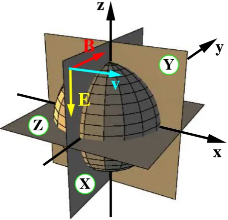
Fig. 1. Plasma environment of Mars – Simulation geometry. The undisturbed plasma flow is directed along the(+x)axis, whereas the homogeneous solar wind magnetic field is parallel to the(+y)axis. Hence, the convective electric field, defining the direction of asymmetry, is oriented antiparallel to thezaxis. The obstacle’s dayside is located in the(x <0)hemisphere. In the figure, the cutting planes(x= 0),(y= 0)and(z= 0)are denoted by the abbreviations X,YandZ, respectively.
Fig. 1. Plasma environment of Mars – Simulation geometry. The undisturbed plasma flow is directed along the (+x)-axis, whereas the homogeneous solar wind magnetic field is parallel to the (+y)-axis. Hence, the convective electric field, defining the direction of asym-metry, is oriented antiparallel to the z-axis. The obstacle’s dayside
is located in the(x<0)hemisphere. In the figure, the cutting planes
(x=0),(y0)and(z0)are denoted by the abbreviations X, Y and Z,
respectively.
3 The Martian plasma environment (MA>1, MS>1,
MMS>1)
In order to illustrate the Martian interaction with the so-lar wind, a 3-D hybrid simulation has been carried out. The simulation geometry is displayed in Fig. 1: the undis-turbed solar wind density and magnetic field are given by nSW,0=4 cm−3andBSW,0=(0,3 nT,0), respectively. The
upstream plasma flow is directed parallel to the (+x)-axis, the upstream alfv´enic Mach number is set toMA=10. As
the electron and proton temperatures in the undisturbed so-lar wind have been set toTe=2×10⁵ K andTp=5×10⁴ K,
the corresponding plasma betas in the undisturbed flow are βe=3.1 andβi=0.8. This yields values of
MS =
MA q
κ
2(βe+βi)
=5.1 (6)
and MMS =
MA q
κ
2(βe+βi)+1
=4.5 (7)
for the sonic and the magnetosonic Mach number, respec-tively.
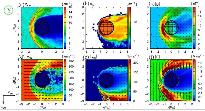
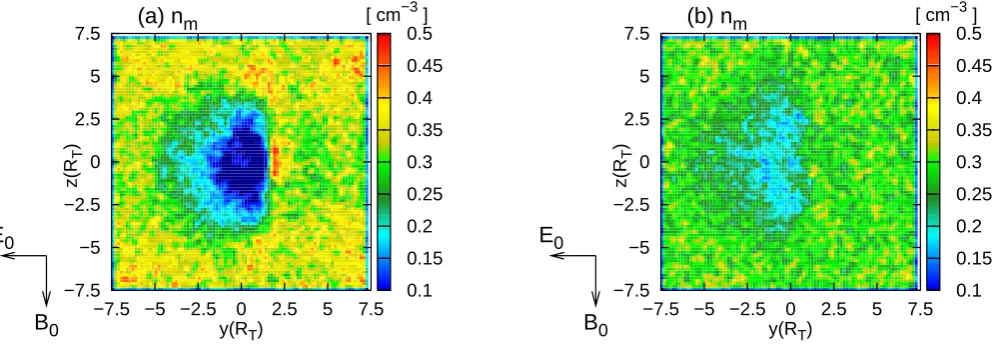
Figure 2 displays the simulation results for the polar plane, coinciding with the(x, z)plane of the coordinate system. It
can be seen in Figs. 2a and b that downstream of the bow shock, the decelerated solar wind is clearly separated from the ionospheric plasma flow by means of an Ion Composi-tion Boundary, i.e. the solar wind density is high in regions where the ionospheric density is low and vice versa. It is obvious that the structure of the ionospheric tail as well as the magnetic pile-up region at the Martian dayside exhibit a pronounced asymmetry with respect to the direction of the convective electric field.
In the following, we will try to understand the mechanism giving rise to the Ion Composition Boundary by means of a kinetic approach, i.e. by considering the Lorentz forces act-ing on individual ions of solar wind and ionospheric origin. These forces are given by
FSW =e (E+vSW×B) (8) for a solar wind particle and by
FH I =e (E+vH I ×B) (9)
for a heavy ion of ionospheric origin. For the formation of the Ion Composition Boundary, two different contributions to the electric field are of major importance: On the one hand, this is the convective electric field term
Ec= −ui×B . (10)
By introducing the average densitiesnSWandnH I of the
so-lar wind and the heavy ion component, this term can be writ-ten as
Ec=
= −
n
SW
nSW+nH I
uSW+ nH I
nSW+nH I
uH I
×B ,
(11) whereuSW anduH I denote the bulk velocities of the
so-lar wind and the heavy ion component, respectively. As can be seen from Eq. (11), the convective electric field is dom-inated by the fast solar wind velocity in regions where the ionospheric ion density is small, whereas in regions of high heavy ion density, the slow velocityuH Igives the major con-tribution to the convective electric field.
On the other hand, the electron pressure terms are of im-portant consequence for the formation of the Ion Composi-tion Boundary:
E∇ = −
∇Pe,SW+ ∇Pe,H I
e(ne,SW+ne,H I)
. (12)
[image:4.595.50.282.64.287.2](c)
(b)
(a)
(f)
(e)
(d)
[image:5.595.84.509.64.293.2]Y
Fig. 2. Plasma environment of Mars – Results of a 3-D hybrid simulation. The figure shows a cut through the polar plane. The quantities displayed in the figure are (a) the solar wind density, (b) the ionospheric heavy ion density, (c) the magnetic field, (d) the solar wind velocity, (e) the heavy ion velocity and (f) the electric field. In the Martian scenario the individual particle velocitiesvSW in the upstream flow
do not differ significantly from the mean plasma velocitiesuSW. Therefore, the arrowvSW on the left side of the figure denotes both a
representative particle velocity and the mean plasma velocity. Mach numbers of the upstream plasma flow: MA=10.0 (alfv´enic),MS=5.1
(sonic) andMMS=4.5 (magnetosonic).
For instance, in regions where the solar wind particles are predominant, one obtains
E∇ ≈ −
∇Pe,SW
ene,SW
=
= −κ ne,SW
κ−1∇ ne,SW
ene,SW
= −2∇ne,SW
e . (13)
It is interesting to notice that this term depends only on the density gradient ∇ne,SW, but not on the absolute density
valuene,SW.
Outside the ionospheric tail region, the solar wind ions are the predominant species. For this reason, the convective elec-tric field outside the tail can be written as
Ec≈ −uSW ×B . (14)
Now we consider the situation near the flank of the iono-spheric tail in the northern hemisphere of the polar plane, referring to a heavy ion that is about to enter the proton-dominated plasma flow from inside the tail region. The heavy ion trys to cross the tail’s northern boundary from inward to outward. As the individual velocityvH I of such a heavy
ion is significantly smaller than the flow velocity of the solar wind, the Lorentz force acting on the particle is given by FH I =e
(vH I−uSW)×B−
2∇ne,SW
e
≈e
−uSW×B−
2∇ne,SW
e
. (15)
Due to the relatively high velocity of the shocked solar wind in this region (cf. Fig. 2d) and the magnetic field enhance-ment in the lobes (cf. Yeroshenko et al., 1990; B¨oßwetter et al., 2004), the first term including the magnetic field is the predominat one, i.e.
FH I ≈ −euSW×B. (16)
104 S. Simon et al.: Physics of the Ion Composition Boundary 0 0.5 1 1.5 2 Bsw Esw z(R M )
⎪E + vsw× B⎪/ (vsw,0 B0)
3 2 1 0 −1 −2 −3
y(RM) 3 2 1 0 −1 −2
−3 0
0.5 1 1.5 2
⎪E + vhi× B⎪/ (vsw,0 B0)
3 2 1 0 −1 −2 −3
y(RM) 3 2 1 0 −1 −2 −3 0 0.5 1 1.5 2 vsw Esw z(R M )
⎪E + vsw× B⎪/ (vsw,0 B0)
3 2 1 0 −1 −2 −3
x(RM) 3 2 1 0 −1 −2
−3 0
0.5 1 1.5 2
⎪E + vhi× B⎪/ (vsw,0 B0)
3 2 1 0 −1 −2 −3
x(RM) 3 2 1 0 −1 −2 −3 0 0.5 1 1.5 2 vsw Bsw y(R
M
)
⎪E + vsw× B⎪/ (vsw,0 B0)
3 2 1 0 −1 −2 −3
x(RM) 3 2 1 0 −1 −2
−3 0
0.5 1 1.5 2
⎪E + vhi× B⎪/ (vsw,0 B0)
3 2 1 0 −1 −2 −3
[image:6.595.126.467.72.475.2]x(RM) 3 2 1 0 −1 −2 −3 3 2 1 0 −1 −2 −3 3 2 1 0 −1 −2 −3 3 2 1 0 −1 −2 −3 3 2 1 0 −1 −2 −3 3 2 1 0 −1 −2 −3 3 2 1 0 −1 −2 −3 3 2 1 0 −1 −2 −3 3 2 1 0 −1 −2 −3 3 2 1 0 −1 −2 −3 3 2 1 0 −1 −2 −3 3 2 1 0 −1 −2 −3 3 2 1 0 −1 −2 −3
(f)
(d)
(b)
(c)
(a)
(e)
X
Y
Z
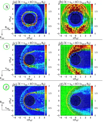
Fig. 3. Plasma environment of Mars – Lorentz forces. The figure diplays the Lorentz forces acting on solar wind (SW) and ionospheric
heavy ions (H I) for the terminator plane: (a) and (b), the polar plane: (c) and (d), and the equatorial plane: (e) and (f). The arrows denote
the projection of the force vectors on the cutting planes. The Lorentz force is given in units ofvSW,0B0, i.e. the quantity displayed in the
figure is dimensionless. The cutting planes(x=0),(y=0)and(z0)are denoted by the abbreviations X, Y and Z, respectively. Mach numbers
of the upstream plasma flow:MA=10.0 (alfv´enic),MS=5.1 (sonic) andMMS=4.5 (magnetosonic).
In an analogeous manner, one can discuss the dynamics of a solar wind proton in the northern hemisphere of the po-lar plane, attempting to cross the Ion Composition Bound-ary from outward to inward. When trying to get into the tail region, the proton velocityvSW is approximately the ion
bulk velocityuSW, so that the convective electric field in the
Lorentz force equation cancels with thevSW×Bterm.
Con-sequently, the force acting on the particle is clearly domi-nated by the two electron pressure terms. As the solar wind density inside the tail is almost zero, the major force acting on the proton arises from the ionospheric density gradient
near the northern flank of the tail: FSW = −e
∇(ne,SW)κ+ ∇(ne,H I)κ
e(ne,SW+ne,H I)
≈ −2∇ne,H I . (17)
Inside the ionospheric tail itself, the solar wind particles are only of minor importance. As the mean heavy ion ve-locityuH I inside the tail region does not differ significantly
from the individual particle velocitiesvH I and the magnetic
field is weak, the forces acting on the heavy ions inside the tail region are mainly governed by local density gradients, i.e.
FH I ≈ −2e
∇ne,H I
e . (18)
Since according to Fig. 2b no strong density gradients occur in the central tail region beyond the obstacle, the characteris-tic time scale for the motion of the heavy ions is very large.
The kinetic approach discussed above also allows to ex-plain the lack of an ICB in the southern hemisphere. In this hemispere, the convective electric field is directed away from the obstacle. Therefore, it drags the ionospheric particles away from Mars, giving rise to an extended pick-up region (cf. Fig. 2e). At the tail’s outer flank in this hemisphere, both the electric field arising from the electron density gradi-ent and the convective electric field are directed away from Mars, i.e. the vectors are antiparallel to the z-axis. Due to the anti-parallelism of both forces being the essential condition for the formation of the Ion Composition Boundary, such a boundary layer is not formed in the southern hemisphere.
The highly asymmetric structure of the ionospheric tail and the ICB surrounding it is not only confirmed by other simulation studies (B¨oßwetter et al., 2004; Modolo et al., 2005), but also by observations. The existence of an asym-metry is suggested by Vennerstrom et al. (2003) who con-ducted a statistical analysis of the magnetic field data col-lected by MGS. The same phenomenon is discussed by Brain et al. (2005, 2006). However, a detailed global data analysis concerning the formation of the ICB has not yet been per-formed. Due to permanent changes in the direction of the solar wind magnetic field and therefore in the direction of the convective electric field, carrying out such an analysis is extremely difficult. Therefore, even though the decisive role of the electric field direction has already been emphasized by numerical models, including this aspect into data analysis will be left to future work.
The qualitative discussion that has been given above is in complete agreement to the results of our simulation model. In order to demonstrate this, the Lorentz forces acting on so-lar wind and ionospheric heavy ions are displayed in Fig. 3, not only for the polar plane, but also for cuts through the ter-minator plane and the equatorial plane. As shown in Figs. 3a, c and e, in the vicinity of Mars the Lorentz forces acting on solar wind protons are always directed away from the ob-stacle. A sudden increase of Lorentz force strength mani-fests in all three cutting planes, denoting the position of the Ion Composition Boundary. It is obvious that the deflection of the ionospheric particles away from Mars occurs primar-ily in these regions. As can be seen in Figs. 3b and d, in the northern hemisphere where the undisturbed convective
0
0
u
0
B
Sunlight
To Saturn
z
y
x
[image:7.595.309.541.62.268.2]E
Fig. 4. Plasma environment of Titan – Simulation geometry.
The dayside of the obstacle is located in the(x<0)hemisphere.
The undisturbed plasma flow is directed parallel to the (+x)-axis, whereas the undisturbed Saturnian magnetic field is perpendicular
to Titan’s orbital plane, pointing in (−z)-direction. When Titan is
located inside Saturn’s magnetosphere, the y-axis is pointing to-wards Saturn. The boundary layer denoted by the red lines is located
in Titan’s wake region. In this geometry, the(x, y)plane of the
co-ordinate system coincides with Titan’s equatorial plane, whereas
the polar plane is identical to the(x, z)plane. This situation differs
from the Martian simulation geometry displayed in Fig. 1.
electric field is pointing in the direction of the (−z)-axis, the Lorentz force acting on particles of ionospheric origin is al-ways oriented towards Mars. This yields a sharp confinement of the ionospheric particles to the near-obstacle region. In the southern hemisphere, the convective electric field is directed away from the obstacle. Correspondingly, the Lorentz forces acting on ionospheric particles are pointing away from Mars in the southern hemisphere of the terminator plane, as dis-played in Fig. 3b. Since the Lorentz forces acting on the two different ion species are parallel in this hemisphere, an Ion Composition Boundary cannot be formed. As displayed in Fig. 3d, an analogeus process occurs in the southern hemi-sphere of the polar plane. However, it is also obvious that in this hemisphere, the Lorentz force on ionospheric oxygen ions possesses a component parallel to the direction of the undisturbed solar wind flow, cleary illustrating the pick-up of these particles.
Finally, it should be noticed that the second term in Eq. (2) is of no consequence for the discussion of the asymmetries in the wake region of the polar plane. The numerator of this term can be expressed as
(∇ ×B)×B= −1
2∇B
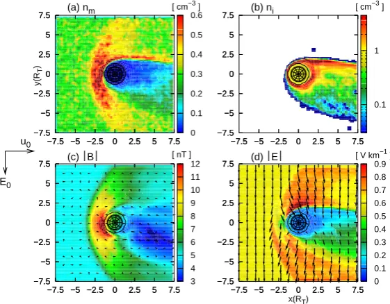
106 S. Simon et al.: Physics of the Ion Composition Boundary 0 0.1 0.2 0.3 0.4 0.5 0.6 u0 B0
(a) nm [ cm−3 ]
z(R T ) 7.5 5 2.5 0 −2.5 −5 −7.5 7.5 5 2.5 0 −2.5 −5 −7.5 0.1 1
(b) ni [ cm−3 ]
7.5 5 2.5 0 −2.5 −5 −7.5 7.5 5 2.5 0 −2.5 −5 −7.5 3 4 5 6 7 8 9 10 11 12
(c) ⎪B⎪ [ nT ]
7.5 5 2.5 0 −2.5 −5 −7.5 7.5 5 2.5 0 −2.5 −5
−7.5 0
0.1 0.2 0.3 0.4 0.5 0.6 0.7 0.8 0.9
(d) ⎪E⎪ [ V km−1 ]
7.5 5 2.5 0 −2.5 −5 −7.5
x(RT)
[image:8.595.155.436.62.281.2]7.5 5 2.5 0 −2.5 −5 −7.5 7.5 5 2.5 0 −2.5 −5 −7.5 7.5 5 2.5 0 −2.5 −5 −7.5 7.5 5 2.5 0 −2.5 −5 −7.5 7.5 5 2.5 0 −2.5 −5 −7.5 7.5 5 2.5 0 −2.5 −5 −7.5 7.5 5 2.5 0 −2.5 −5 −7.5 7.5 5 2.5 0 −2.5 −5 −7.5 7.5 5 2.5 0 −2.5 −5 −7.5
Fig. 5. Titan’s interaction with a slightly super-alfv´enic, supersonic and supermagnetosonic plasma flow – Cut through the polar plane. The figure displays (a) the ambient plasma density, (b) the ionospheric plasma density and the electromagnetic fields: (c) and (d). Mach numbers
of the upstream plasma flow:MA=1.87 (alfv´enic),MS=2.9 (sonic) andMMS=1.6 (magnetosonic).
0 0.1 0.2 0.3 0.4 0.5 0.6 u0 E0
(a) nm [ cm
−3 ] y(R T ) 7.5 5 2.5 0 −2.5 −5 −7.5 7.5 5 2.5 0 −2.5 −5 −7.5 0.1 1
(b) ni [ cm
−3 ] 7.5 5 2.5 0 −2.5 −5 −7.5 7.5 5 2.5 0 −2.5 −5 −7.5 3 4 5 6 7 8 9 10 11 12
(c) ⎪B⎪ [ nT ]
7.5 5 2.5 0 −2.5 −5 −7.5 7.5 5 2.5 0 −2.5 −5
−7.5 0
0.1 0.2 0.3 0.4 0.5 0.6 0.7 0.8 0.9
(d) ⎪E⎪ [ V km−1 ]
7.5 5 2.5 0 −2.5 −5 −7.5
x(RT)
7.5 5 2.5 0 −2.5 −5 −7.5 7.5 5 2.5 0 −2.5 −5 −7.5 7.5 5 2.5 0 −2.5 −5 −7.5 7.5 5 2.5 0 −2.5 −5 −7.5 7.5 5 2.5 0 −2.5 −5 −7.5 7.5 5 2.5 0 −2.5 −5 −7.5 7.5 5 2.5 0 −2.5 −5 −7.5 7.5 5 2.5 0 −2.5 −5 −7.5 7.5 5 2.5 0 −2.5 −5 −7.5
Fig. 6. Titan’s interaction with slightly super-alfv´enic, supersonic and supermagnetosonic plasma flow – Cut through the equatorial plane.
The physical quantities shown in the figure are the same as in Fig. 5. Mach numbers of the upstream plasma flow: MA=1.87 (alfv´enic),
MS=2.9 (sonic) andMMS=1.6 (magnetosonic).
showing that it is determined by the magnetic pressure gradi-ent as well as the magnetic tension in regions of curved mag-netic field lines. The magmag-netic pressure term plays an im-portant role for the structure of the magnetic pile-up region at the Martian ramside. Besides, magnetic pressure effects have a decisive character for the structure of the magnetic lobes. However, neither of these two forces is important for
[image:8.595.155.436.346.565.2]0.2 0.25 0.3 0.35 0.4 u0 B0
(a) nm [ cm−3 ]
z(R T ) 7.5 5 2.5 0 −2.5 −5 −7.5 7.5 5 2.5 0 −2.5 −5 −7.5 0.1 1
(b) ni [ cm−3 ]
7.5 5 2.5 0 −2.5 −5 −7.5 7.5 5 2.5 0 −2.5 −5 −7.5 3 4 5 6 7 8 9 10 11 12
(c) ⎪B⎪ [ nT ]
7.5 5 2.5 0 −2.5 −5 −7.5 7.5 5 2.5 0 −2.5 −5
−7.5 0
0.1 0.2 0.3 0.4 0.5 0.6 0.7 0.8 0.9
(d) ⎪E⎪ [ V km−1 ]
7.5 5 2.5 0 −2.5 −5 −7.5
x(RT)
[image:9.595.155.437.61.281.2]7.5 5 2.5 0 −2.5 −5 −7.5 7.5 5 2.5 0 −2.5 −5 −7.5 7.5 5 2.5 0 −2.5 −5 −7.5 7.5 5 2.5 0 −2.5 −5 −7.5 7.5 5 2.5 0 −2.5 −5 −7.5 7.5 5 2.5 0 −2.5 −5 −7.5 7.5 5 2.5 0 −2.5 −5 −7.5 7.5 5 2.5 0 −2.5 −5 −7.5 7.5 5 2.5 0 −2.5 −5 −7.5
Fig. 7. Interaction between Titan’s ionosphere and a slightly super-alfv´enic, yet subsonic and submagnetosonic plasma flow – Cut through
the polar plane. The physical quantities shown in the figure are the same as in Fig. 5. Mach numbers of the upstream plasma flow:MA=1.87
(alfv´enic),MS=0.57 (sonic) andMMS=0.55 (magnetosonic).
0.2 0.25 0.3 0.35 0.4 u0 E0
(a) nm [ cm
−3 ] y(R T ) 7.5 5 2.5 0 −2.5 −5 −7.5 7.5 5 2.5 0 −2.5 −5 −7.5 0.1 1
(b) ni [ cm
−3 ] 7.5 5 2.5 0 −2.5 −5 −7.5 7.5 5 2.5 0 −2.5 −5 −7.5 3 4 5 6 7 8 9 10 11 12
(c) ⎪B⎪ [ nT ]
7.5 5 2.5 0 −2.5 −5 −7.5 7.5 5 2.5 0 −2.5 −5
−7.5 0
0.1 0.2 0.3 0.4 0.5 0.6 0.7 0.8 0.9
(d) ⎪E⎪ [ V km−1 ]
7.5 5 2.5 0 −2.5 −5 −7.5
x(RT)
7.5 5 2.5 0 −2.5 −5 −7.5 7.5 5 2.5 0 −2.5 −5 −7.5 7.5 5 2.5 0 −2.5 −5 −7.5 7.5 5 2.5 0 −2.5 −5 −7.5 7.5 5 2.5 0 −2.5 −5 −7.5 7.5 5 2.5 0 −2.5 −5 −7.5 7.5 5 2.5 0 −2.5 −5 −7.5 7.5 5 2.5 0 −2.5 −5 −7.5 7.5 5 2.5 0 −2.5 −5 −7.5
Fig. 8. Interaction between Titan’s ionosphere and a slightly super-alfv´enic, yet subsonic and submagnetosonic plasma flow – Cut through the equatorial plane. The physical quantities shown in the figure are the same as in Fig. 5. Mach numbers of the upstream plasma flow:
MA=1.87 (alfv´enic),MS=0.57 (sonic) andMMS=0.55 (magnetosonic).
chosen by Bagdonat (2004). The importance of magnetic ef-fects for the ionospheric tail structure in the equatorial plane, containing the highly curved field lines, has been discussed by B¨oßwetter et al. (2004).
4 Titan in the solar wind (MA>1,MS>1,MMS>1)
[image:9.595.155.436.345.564.2]108 S. Simon et al.: Physics of the Ion Composition Boundary plasma environment undergoes when the satellite re-enters
the magnetosphere. Therefore, four different simulation sce-narios have been considered. At first, the case of Titan being exposed to a slightly super-alfv´enic (MA=1.87), supersonic
(MS=2.9) and supermagnetosonic (MMS=1.6) plasma flow
has been analyzed. Even though the Mach numbers are sig-nificantly smaller and closer to 1 than in the Martian sce-nario, the global features of the interaction region in both cases should exhibit many similarities. Secondly, the inter-action between Titan’s ionosphere and the plasma in Saturn’s outer magnetosphere has been analyzed. In this scenario, the upstream flow is super-alfv´enic, yet subsonic and submagne-tosonic.
A third geometry which is characterized by a super-alfv´enic and supersonic, yet submagnetosonic flow, illus-trates the transition between the situation outside and inside the magnetosphere. A fourth geometry refers to the case of Titan being located in Saturn’s magnetotail.
In order to allow a direct comparison between the re-sults, the upstream plasma flow is assumed to be consist-ing of a sconsist-ingle ion species of massm=9.6 amu and density nm=0.3 cm−3in all four simulations. These parameters are
average values for a plasma consisting of nitrogen (N+) and hydrogen (H+) ions and can be obtained from the Voyager 1 data (Kallio et al., 2004; Backes et al., 2005; Simon et al., 2006b). In the following, this plasma is referred to as the (N+/H+) plasma.
The simulation geometry is displayed in Fig. 4. The (+x)-axis is pointing from the Sun to Titan, whereas the undis-turbed background magnetic fieldB0=(0,0,−5 nT)is
ori-ented antiparallel to the z-axis. The undisturbed plasma ve-locityu0=(120 km/s,0,0)is directed parallel to the x-axis.
Of course, these parameters do not represent real solar wind conditions and have been chosen to achieve the same charac-teristic plasma scales for the situation inside and outside the magnetosphere. This supersonic scenario has simply been generated from the case of Titan being located inside the magnetosphere by reducing the plasma temperature, all other upstream parameters are the same. Especially the plasma composition does not represent real solar wind conditions. However, as this case will only provide a qualitative refer-ence to understand Titan’s interaction with Saturn’s magne-tospheric plasma, it is only of minor quantitative interest. A similar approach to identify the global characteristics of Ti-tan’s interaction with a supersonic flow has been chosen by Kabin et al. (1999, 2000); Kallio et al. (2004) and Simon et al. (2006b).
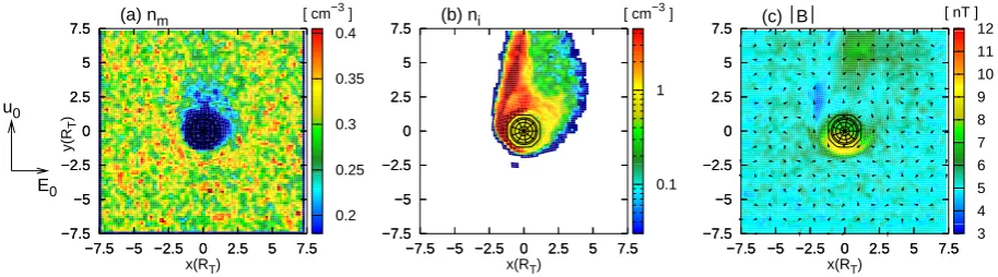
For the case of all three Mach numbers being larger than 1, a plot of the ambient (nm) and ionospheric (ni) ion
densi-ties as well as the electromagnetic field quantidensi-ties is given in Figs. 5 and 6, respectively.
The major features of the interaction region are quite sim-ilar to the Martian plasma environment. A sharply pro-nounced bow wave arises in front of the obstacle, denoting a sudden decrease of plasma velocity. In the plane
perpen-dicular to the convective electric field, the structure of the interaction region is highly symmetric (cf. Fig. 5), whereas an asymmetry with respect to the direction of the convective electric field is formed in the equatorial plane. In the polar plane, a cone-shaped wake region is formed downstream of the obstacle, denoting a significant decrease of the ambient plasma density. In strong analogy, the ionospheric particle density is high inside the cone-shaped wake region, whereas it vanishes outside the tail. The mechanism giving rise to the asymmetries in the structure of the Ion Composition Bound-ary is well illustrated by the cut through the equatorial plane (cf. Fig. 6). In the(y>0)hemisphere, where the convective electric field points towards Titan, a sharp increase of iono-spheric plasma density manifests near the outer flank of the ionospheric tail. This gives rise to a fieldE∝−∇Pe.
There-fore, the (N+/H+) ions which are dragged against this
bar-rier from outside by the convective electric field are unable to pass this region, yielding a line-like region of increased (N+/H+) density near the outer flank of the boundary layer.
5 Titan in Saturn’s outer magnetosphere (MA>1,
MS<1,MMS<1)
The set of Mach numbers for the case of Titan being located in Saturn’s outer magnetosphere has been chosen in accor-dance to the data collected during the Voyager 1 flyby of Titan (Ness et al., 1982; Backes, 2005): the alfv´enic Mach number is given byMA=1.87, whereas values ofMS=0.57
andMMS=0.55 have been chosen for the sonic and the
mag-netosonic Mach numbers, respectively.
When Titan is located in the outer regions of Saturn’s mag-netosphere, the impinging plasma flow is super-alfv´enic, yet subsonic and submagnetosonic. Consequently, no bow shock will form in front of the obstacle. The simulation results for this scenario are displayed in Fig. 7 for the polar plane and in Fig. 8 for the equatorial plane. As can be seen in Fig. 8b, the structure of the ionospheric tail is still highly asymmetric with respect to the direction of the convective electric field, but however, the magnetospheric plasma (nm) is no longer
separated from the ionospheric plasma flow, i.e. the Ion Com-position Boundary has vanished.
0.2 0.25 0.3 0.35 0.4 u0 B0
(a) nm [ cm−3 ]
z(R T ) 7.5 5 2.5 0 −2.5 −5 −7.5 7.5 5 2.5 0 −2.5 −5 −7.5 0.1 1
(b) ni [ cm−3 ]
7.5 5 2.5 0 −2.5 −5 −7.5 7.5 5 2.5 0 −2.5 −5
−7.5 3
4 5 6 7 8 9 10 11 12
(c) ⎪B⎪ [ nT ]
7.5 5 2.5 0 −2.5 −5 −7.5 7.5 5 2.5 0 −2.5 −5 −7.5 40 60 80 100 120 140 160
(d) ⎪um⎪ [ km s−1 ]
z(R T ) 7.5 5 2.5 0 −2.5 −5 −7.5
x(RT)
7.5 5 2.5 0 −2.5 −5
−7.5 0
20 40 60 80 100 120 140 160 180
(e) ⎪ui⎪ [ km s−1 ]
7.5 5 2.5 0 −2.5 −5 −7.5
x(RT)
7.5 5 2.5 0 −2.5 −5
−7.5 0
0.1 0.2 0.3 0.4 0.5 0.6 0.7 0.8 0.9
(f) ⎪E⎪ [ V km−1 ]
7.5 5 2.5 0 −2.5 −5 −7.5
x(RT)
[image:11.595.83.511.62.291.2]7.5 5 2.5 0 −2.5 −5 −7.5 7.5 5 2.5 0 −2.5 −5 −7.5 7.5 5 2.5 0 −2.5 −5 −7.5 7.5 5 2.5 0 −2.5 −5 −7.5 7.5 5 2.5 0 −2.5 −5 −7.5 7.5 5 2.5 0 −2.5 −5 −7.5 7.5 5 2.5 0 −2.5 −5 −7.5 7.5 5 2.5 0 −2.5 −5 −7.5 7.5 5 2.5 0 −2.5 −5 −7.5 7.5 5 2.5 0 −2.5 −5 −7.5 7.5 5 2.5 0 −2.5 −5 −7.5 7.5 5 2.5 0 −2.5 −5 −7.5 7.5 5 2.5 0 −2.5 −5 −7.5
Fig. 9. Transition from supermagnetosonic to submagnetosonic flow – Cut through the(x, z)plane of the coordinate system which coincides
with Titan’s polar plane. The figure displays the (N+/H+)plasma density and velocity: (a) and (d), the ionospheric ion density and velocity:
(b) und (e), and the electromagnetic fields: (c) and (f). The figure illustrates the transition from the case of Titan being located outside the magnetosphere, where all three Mach numbers are larger than 1, to the case of Titan’s interaction with Saturn’s magnetospheric plasma at
18:00 LT. Mach numbers of the upstream plasma flow:MA=1.87 (alfv´enic),MS=1.08 (sonic) andMMS=0.94 (magnetosonic).
However, as can be seen in Fig. 8b, only a slight decrease of ionospheric plasma density occurs near the outer flank of the ionospheric tail. Due to the adiabatic description of the electron fluid, the electric field arising from the pressure gradient is too weak to prevent the magnetospheric plasma from mixing with the ionospheric plasma flow. For this rea-son, only a minor, but nevertheless still asymmetric decrease of magnetospheric plasma density occurs in the vicinity of the obstacle. The Ion Composition Boundary has completely vanished. In contrast to this, the situation in the(y<0) hemi-sphere is very similar to the case of Titan being loacted out-side of the magnetosphere. The electric field is directed away from the obstacle, leading to the formation of an extended pick-up region. A more extensive discussion for this scenario is given by Simon et al. (2006b). In the following section, we intend to focus on illustrating the physical process that results in the disappearence of the Ion Composition Boundary.
6 Transition from supersonic to subsonic flow (MA>1,MS>1,MMS<1)
In this section, the transition between the two scenarios de-scribed in the preceding sections shall be investigated in more detail. For this reason, another simulation run has been conducted. In order to gain access to the transition between the cases of Titan being located outside and inside the magnetosphere, the upstream plasma flow is assumed to be super-alfv´enic (MA>1) and supersonic (MS>1), yet
sub-magnetosonic (MMS<1). Specifically, values ofMA=1.87,
MS=1.08 and MMS=0.94 have been chosen for the Mach
numbers of the impinging flow, corresponding to values of βe,m=0.97 andβm=2.00 for the (N+/H+) plasma’s electron
and ion betas, respectively. All other simulation parameters, including the upstream plasma composition as well as the background magnetic field and density are the same as in the other Titan simulation runs presented in this work. Even though this situation is not representative for a real situation in Titan’s plasma environment, it will show to be extremely valuable for unterstanding the transition that the obstacle’s plasma environment undergoes.
110 S. Simon et al.: Physics of the Ion Composition Boundary 0.2 0.25 0.3 0.35 0.4 u0 E0
(a) nm [ cm−3 ]
y(R T ) 7.5 5 2.5 0 −2.5 −5 −7.5 7.5 5 2.5 0 −2.5 −5 −7.5 0.1 1
(b) ni [ cm−3 ]
7.5 5 2.5 0 −2.5 −5 −7.5 7.5 5 2.5 0 −2.5 −5
−7.5 3
4 5 6 7 8 9 10 11 12
(c) ⎪B⎪ [ nT ]
7.5 5 2.5 0 −2.5 −5 −7.5 7.5 5 2.5 0 −2.5 −5 −7.5 40 60 80 100 120 140 160
(d) ⎪um⎪ [ km s−1 ]
y(R T ) 7.5 5 2.5 0 −2.5 −5 −7.5
x(RT) 7.5 5 2.5 0 −2.5 −5
−7.5 0
20 40 60 80 100 120 140 160 180
(e) ⎪ui⎪ [ km s−1 ]
7.5 5 2.5 0 −2.5 −5 −7.5
x(RT) 7.5 5 2.5 0 −2.5 −5
−7.5 0
0.1 0.2 0.3 0.4 0.5 0.6 0.7 0.8 0.9
(f) ⎪E⎪ [ V km−1 ]
7.5 5 2.5 0 −2.5 −5 −7.5
[image:12.595.85.507.63.291.2]x(RT) 7.5 5 2.5 0 −2.5 −5 −7.5 7.5 5 2.5 0 −2.5 −5 −7.5 7.5 5 2.5 0 −2.5 −5 −7.5 7.5 5 2.5 0 −2.5 −5 −7.5 7.5 5 2.5 0 −2.5 −5 −7.5 7.5 5 2.5 0 −2.5 −5 −7.5 7.5 5 2.5 0 −2.5 −5 −7.5 7.5 5 2.5 0 −2.5 −5 −7.5 7.5 5 2.5 0 −2.5 −5 −7.5 7.5 5 2.5 0 −2.5 −5 −7.5 7.5 5 2.5 0 −2.5 −5 −7.5 7.5 5 2.5 0 −2.5 −5 −7.5 7.5 5 2.5 0 −2.5 −5 −7.5
Fig. 10. Transition from supermagnetosonic to submagnetosonic flow – Cut through Titan’s equatorial plane which is parallel to the undis-turbed convective electric field. The physical quantities shown in the figure are the same as in Fig. 9. Mach numbers of the upstream plasma
flow:MA=1.87 (alfv´enic),MS=1.08 (sonic) andMMS=0.94 (magnetosonic).
fromn=0.3 cm−3in the undisturbed flow ton=0.4 cm−3in the near-Titan upstream region. However, this structure is not as sharply confined as in the case of Titan being located outside of the magnetosphere.
Besides, a pronounced region of reduced plasma velocity in the downstream region has shown to be characteristic for the interaction region when Titan is exposed to the solar wind, as discussed by Simon et al. (2006b). Such a decrease is still present in the case currently under consideration, as can be seen from Fig. 9d. Although the plasma is still decel-erated, the respective region in the polar plane is not sharply separated from the ambient plasma flow. In the case of Titan being located outside the magnetosphere, the interaction in the polar plane gave rise to a cone-shaped region of reduced (N+/H+) density in the vicinity of Titan, its outer boundaries denoting the position of the Ion Composition Boundary in a plane perpendicular to the undisturbed convective electric fieldE0=−u0×B0. This is displayed in Fig. 5a. An
analo-geous cone-like structure can be seen in Fig. 9a, although the decrease of (N+/H+) density has significantly diminished. Besides, the structure denotes no longer a sharp, but a smooth transition from the plasma inside the cone-shaped region to the ambient plasma flow.
The transition that the tail structure undergoes is also illus-trated in Fig. 11. Plot 11a displays a cut through the tail struc-ture of the supermagnetosonic case, whereas a cut through the tail in the submagnetosonic case is shown in Fig. 11b. Both cutting planes are located atx=+5RT downstream of
Titan. As can be seen in Fig. 11a, in the supermagnetosonic case, the density cavity in the wake exhibits a sharply
pro-nounced boundary along the y=1RT line, i.e. the density
strongly decreases on a characteristic scale below one Titan radius. In contrast to this, when moving away from the ob-stacle in negative y-direction, a quite smooth density increase occurs, illustrating that no sharp boundary layer exists in the (y<0)hemisphere. As can be seen from Fig. 11b, in the sub-magnetosonic case, the structure of the density cavity is still highly asymmetric. However, a smooth transition to the am-bient density does not only occur in the(y<0), but also in the (y>0)hemisphere. The ambient density in the(x=+5RT)
cutting plane is smaller than in the supermagnetosonic case, as the shock denoing an increase of plasma density has van-ished. To sum up, the position of the former Ion Composi-tion Boundary is still identifiable, but the impinging plasma is no longer forbidden to cross this boundary layer and to mix with the ionospheric pick-up ions. A possible reason for this might be the increased plasma temperature, allowing a larger number of particles with high thermal velocity to cross the potential barrier at the tail’s flank. These signatures clearly illustrate the transition to the case of Titan being located in-side Saturn’s magnetosphere, where the boundary layer has completely vanished.
0.1 0.15 0.2 0.25 0.3 0.35 0.4 0.45 0.5
(a) n
m [ cm−3 ]E
0B
0z(R
T
)
7.5 5 2.5 0 −2.5 −5 −7.5
y(RT) 7.5
5
2.5
0
−2.5
−5
−7.5 0.1
0.15 0.2 0.25 0.3 0.35 0.4 0.45 0.5
(b) n
m [ cm−3 ]E
0B
0z(R
T
)
7.5 5 2.5 0 −2.5 −5 −7.5
y(RT) 7.5
5
2.5
0
−2.5
−5
[image:13.595.52.551.58.234.2]−7.5
Fig. 11. Transition from supersonic to subsonic flow. The figure illustrates the transition that the tail structure downstream of the obstacle
undergoes when the magnetosonic Mach number of the upstream plasma flow is reduced fromMMS>1 toMMS<1. (a) displays a cut through
the tail in the supermagnetosonic case at a distance of 5RT to the center of the obstacle, while an analogeous cut for the submagnetosonic
case is shown in (b). The cutting planes are parallel to the(y, z)plane of the coordinate system, i.e. they are located atx=+5RT. Both
figures display the ambient plasma densitynm.
(cf. Fig. 7c). Besides, when Titan is located inside the mag-netosphere, the magnetic pile-up region at Titan’s dayside possesses an extension of only about 1RT in subsolar
di-rection. In contrast to this, when Titan is located outside the magnetosphere, the magnetic pile-up in the shock front possesses an extension around 3RT in subsolar direction, as
displayed in Figs. 5c and 6c. The transition between both cases is illustrated in Fig. 9c. On the one hand, the inter-action leads to the formation of a confined magnetic draping pattern, being similar to the situation when Titan is located inside the magnetosphere at 18:00 LT. On the other hand, a slight increase of magnetic field strength can be noticed at a subsolar distance of around 2−3RT, denoting the position
of the bow shock in the solar wind scenario. Besides, the magnetic enhancement in the two lobes achieves a maximum value of about 7 nT, whereas a value of 9−10 nT is reached when Titan is located in the magnetosphere at 18:00 LT. This implies that in the transition scenario under consideration, the field lines are incapable of draping completely around the obstacle, but develop an intermediate structure between a parabolic, barely confined shock front and a strongly con-fined draping pattern. To summarize the major results for the polar plane, the boundary structures being typical for the interaction region when Titan is located outside the mag-netosphere are still identifiable in the transition scenario. However, the sharpness of the boundaries, especially the Ion Composition Boundary, has clearly diminished.
Nevertheless, the most important aspect of the transi-tion scenario is the transformatransi-tion that the Ion Compositransi-tion Boundary undergoes in the plane parallel to the undisturbed convective electric fieldE0. The situation in this plane, being
highly asymmetric, is displayed in Fig. 10. In the case of
Ti-tan being located outside the magnetosphere, the interaction gives rise to a sharply developed Ion Composition Bound-ary in the(y>0) hemisphere. As can be seen in Fig. 6b, a sharp increase of ionospheric density manifests near the tail’s flank in the(y>0)hemisphere. The ambient (N+/H+) plasma is pressed against the outer flank of the ionospheric tail by the convective electric field, but however, due to the electric field arising from the electron pressure gradient, it is incapable of crossing the boundary from outward to inward. This effect yields a region of increased (N+/H+) plasma den-sity along the flank of the boundary layer. In the case of Titan being located inside the magnetosphere, the region of sharply increased ionospheric density in the(y>0)hemisphere has vanished, as shown in Fig. 8b. Therefore, the two plasma populations are now allowed to mix. The density plots in Figs. 10a and b illustrate the transition between both cases: As the decrease of ionospheric density in the(y>0) hemi-sphere is weaker than in the situation displayed in Fig. 6b, the ionospheric electron pressure gradient has diminished. This is why the ambient (N+/H+) plasma is capable of gaining ac-cess to the ionospheric tail region. Nevertheless, the former position of the boundary is still identifiable.
7 Titan in Saturn’s magnetotail (MA<1, MS<1,
MMS<1)
112 S. Simon et al.: Physics of the Ion Composition Boundary 0.2 0.25 0.3 0.35 0.4 u0 B0
(a) nm [ cm−3 ]
z(R T ) 7.5 5 2.5 0 −2.5 −5 −7.5
y(RT) 7.5 5 2.5 0 −2.5 −5 −7.5 0.1 1
(b) ni [ cm−3 ]
7.5 5 2.5 0 −2.5 −5 −7.5
y(RT) 7.5 5 2.5 0 −2.5 −5
−7.5 3
4 5 6 7 8 9 10 11 12
(c) ⎪B⎪ [ nT ]
7.5 5 2.5 0 −2.5 −5 −7.5
[image:14.595.70.524.57.183.2]y(RT) 7.5 5 2.5 0 −2.5 −5 −7.5 7.5 5 2.5 0 −2.5 −5 −7.5 7.5 5 2.5 0 −2.5 −5 −7.5 7.5 5 2.5 0 −2.5 −5 −7.5 7.5 5 2.5 0 −2.5 −5 −7.5 7.5 5 2.5 0 −2.5 −5 −7.5 7.5 5 2.5 0 −2.5 −5 −7.5
Fig. 12. Titan’s interaction with the sub-alfv´enic, subsonic and submagnetosonic plasma flow in Saturn’s magnetotail region – Cut through the polar plane. The figure displays (a) the magnetospheric plasma density, (b) the ionospheric plasma density, and (c) the magnetic field.
Mach numbers of the upstream plasma flow:MA=0.77 (alfv´enic),MS=0.27 (sonic) andMMS=0.22 (magnetosonic).
0.2 0.25 0.3 0.35 0.4 E0 u0
(a) nm [ cm−3 ]
y(R T ) 7.5 5 2.5 0 −2.5 −5 −7.5
x(RT) 7.5 5 2.5 0 −2.5 −5 −7.5 0.1 1
(b) ni [ cm−3 ]
7.5 5 2.5 0 −2.5 −5 −7.5
x(RT) 7.5 5 2.5 0 −2.5 −5
−7.5 3
4 5 6 7 8 9 10 11 12
(c) ⎪B⎪ [ nT ]
7.5 5 2.5 0 −2.5 −5 −7.5
x(RT) 7.5 5 2.5 0 −2.5 −5 −7.5 7.5 5 2.5 0 −2.5 −5 −7.5 7.5 5 2.5 0 −2.5 −5 −7.5 7.5 5 2.5 0 −2.5 −5 −7.5 7.5 5 2.5 0 −2.5 −5 −7.5 7.5 5 2.5 0 −2.5 −5 −7.5 7.5 5 2.5 0 −2.5 −5 −7.5
Fig. 13. Titan’s interaction with the sub-alfv´enic, subsonic and submagnetosonic plasma flow in Saturn’s magnetotail region – Cut through the equatorial plane. The figure displays (a) the magnetospheric plasma density, (b) the ionospheric plasma density, and (c) the magnetic
field. Mach numbers of the upstream plasma flow:MA=0.77 (alfv´enic),MS=0.27 (sonic) andMMS=0.22 (magnetosonic).
Simon et al. (2006b). However, as the Cassini flybys take place in late southern summer, a scenario where the obstacle is not completely protected from solar UV ionization might be more realistic. For this reason, the(x<0)hemisphere of Titan is still assumed to be exposed to solar UV radiation. Of course, the geometry of the Cassini flybys is significantly more complex, i.e. Titan’s orbital plane is not parallel to the Sun-Titan-line. Therefore, the real situation of Titan being located inside Saturn’s magnetotail during the Cassini flybys may probably be located between the case discussed here and the scenario of a completely shielded obstacle, as suggested by Simon et al. (2006b). Here, our primary purpose is to keep the simulation geometry as simple as possible to get a good insight into the relevant plasma processes.
The x-axis is again directed from the Sun to Titan, whereas the undisturbed magnetic field is oriented in (−z)-direction. However, in this scenario, the undisturbed plasma flow ve-locity is parallel to the y-axis. Even though this geometry does not represent the real complexity of the situation in late southern summer, it may be considered a closer approxima-tion to the real situaapproxima-tion than the scenario discussed by Simon et al. (2006b). Besides, by retaining the original ionospheric Chapman profile, it is evident that any changes in the
struc-ture of the interaction region will occur due to the altered Mach numbers of the upstream flow. For the simulation, the Mach numbers in the undisturbed plasma have been set to MA=0.77,MS=0.29 andMMS=0.27. The results for the
po-lar plane are displayed in Fig. 12, whereas Fig. 13 shows the results for Titan’s equatorial plane.
[image:14.595.68.525.239.366.2]electric field, but the outer boundary of the ionospheric tail does not manifest in the magnetospheric plasma density (cf. Fig. 13a). Even though a region of enhanced ionospheric plasma density is formed near the outer flank of the tail, the density gradient in this region (i.e. the decrease of iono-spheric plasma density per unit length) is not as sharp as in the case of Titan’s interaction with a supersonic, super-alfv´enic and supermagnetosonic flow (cf. Figs. 6b and 13b). However, the maximum density value that is reached near the outer flank of the tail is almost the same in both scenar-ios. The absolute density value is not of major importance for the effects occuring at the flank of the tail.
8 Summary
In this paper, the plasma environments of Mars and Titan have been studied by means of global, 3-D hybrid simula-tions. Emphasis has been placed on the physical mecha-nism leading to the formation of a so-called Ion Composi-tion Boundary, separating the ionospheric plasma populaComposi-tion from the ambient plasma flow. The physical effects giving rise to such a structure have been investigated as a function of the alfv´enic, sonic and magnetosonic Mach numbers of the upstream plasma flow. In the following, the major results will be summarized by discussing the transition that the ob-stacle’s plasma environment undergoes when the values of the three Mach numbers are reduced from very high values (plasma environment of Mars) to very low values (Titan in Saturn’s magnetotail).
In the Martian situation, the ionospheric plasma flow is clearly separated from the solar wind by a sharphy developed boundary layer which is reproduced by simulations as well as by spacecraft measurements. This boundary layer is highly symmetric in a plane perpendicular to the convective electric field, whereas it exhibits a pronounced asymmetry with re-spect to the direction of this field. The underlying physical mechanism has been explained in terms of a kinetic model, considering the Lorentz forces that act on ions of solar wind and ionospheric origin. The major element of this intepreta-tion is a combinaintepreta-tion of convective electric field and electron pressure forces, leading to the formation of a sharply pro-nounced boundary layer in the hemisphere where both forces are antiparallel. In the hemisphere where the two forces are parallel, the ionospheric particles are dragged away from the obstacle, leading to a significant extension of the ionospheric tail. These considerations are valid for the Martian plasma environment as well as for the case of Titan being exposed to a slightly super-alfv´enic, supersonic and supermagnetosonic plasma flow.
When Titan is exposed to the plasma flow in Saturn’s outer magnetosphere, the ionospheric tail is still asymmetric with respect to the direction of the electric field. However, the boundary layer between both plasma populations has almost vanished because the electron pressure gradient has
signif-icantly diminished. For this reason, it is unable to prevent both plasma populations from mixing. The transition be-tween Titan’s plasma environment outside and inside Sat-urn’s magnetosphere has been illustrated by means of a third scenario, assuming the upstream flow to be super-alfv´enic, supersonic and submagnetosonic. In this geometry, the for-mer position of the Ion Composition Boundary is still identi-fiable, although its sharpness has clearly diminished and both plasmas start mixing. The simulation results clearly illus-trate that the slower is the upstream flow, the less pronounced is the separation of ionospheric and magnetospheric plasma flow. This tendency also manifests in the results for Titan be-ing located in Saturn’s magnetotail, where the upstream flow is sub-alfv´enic, subsonic and submagnetosonic.
To sum up, based on our simulation results, it seems that only in a Mach number regime of 1≤MA a more or less
sharply pronounced Ion Composition Boundary is formed due to the interaction of an unmagnetized planet’s ionosphere with its plasma environment. If the alfv´enic Mach number is smaller, the influence of the convective electric field, caus-ing the asymmetry in the tail structure, does not undergo a significant change. However, as the sharpness of the iono-spheric tail’s outer boundary clearly diminishes, the electric force ramp arising form the−∇Pe term is unable to forbid
the ambient flow to enter the tail region.
On the one hand, our future work will focus on analyz-ing the early Martian plasma environment, especially to ob-tain a comparison to the present situation. Besides, it will be interesting to analyze how the position and structure of the ICB are affected by the strong crustal anomalies at Mars. Harnett and Winglee (2003, 2005) who studied the influence of these anomalies by using a non-ideal MDH model sug-gest that these anomalies do not only cause a local modifica-tion of the boundary layers, but cause a strong distorsion of the ionospheric tail structure on a characteristic length scale of several planetary radii. Since the influence of the mag-netic anomalies has not yet been considered by the hybrid ap-proach, such a modification of the existing simulation model will be realized in the near future.
On the other hand, the analysis of Titan’s plasma environ-ment shall be continued, the simulation geometry matching the situation during specific Cassini flybys. An extension of the model to multispecies upstream conditions will be a first step in this direction.
Acknowledgements. This work has been supported by the Deutsche Forschungsgemeinschaft through the grants MO 539/13-1 and MO 539/ 15-1. Besides, the authors thank J. Schuele from the Institute for Scientific Computing, TU Braunschweig, for numerous valu-able discussions concerning the parallelization of the 3-D simula-tion code.
114 S. Simon et al.: Physics of the Ion Composition Boundary References
Acu˜na, M. H., Connerney, J. E. P., Wasilewski, P., Lin, R. P., Ander-son, K. A., CalAnder-son, C. W., McFadden, J., Curtis, D. W., Mitchell, D., R`eme, H., Mazelle, C., Sauvaud, J. A., d’Uston, C., Cros, A., Medale, J. L., Bauer, S. J., Cloutier, P., Mayhew, M., Winterhal-ter, D., and Ness, N. F.: Magnetic field and plasma observations at Mars: Initial results of the Mars Global Surveyor Mission, Sci-ence, 279, 1676–1680, 1998.
Backes, H.: Titan’s Interaction with the Saturnian Magnetospheric Plasma, Ph.D. thesis, Universit¨at K¨oln, 2005.
Backes, H., Neubauer, F. M., Dougherty, M. K., Achilleos, N., Andr´e, N., Arridge, C. S., Bertucci, C., Jones, G. H., Khurana, K. K., Russell, C. T., and Wennmacher, A.: Titan’s Magnetic Field Signature During the First Cassini Encounter, Science, 308, 992–995, 2005.
Bagdonat, T.: Hybrid Simulation of Weak Comets, Ph.D. thesis, Technische Universit¨at Braunschweig, 2004.
Bagdonat, T. and Motschmann, U.: 3D hybrid simulation of solar wind interaction with comets, in: Space Plasma Simulation – Proceedings of the Sixth International School/ Symposium ISSS-6, edited by: B¨uchner, J., Dum, C., and Scholer, M., 80–83, 2001.
Bagdonat, T. and Motschmann, U.: 3D Hybrid Simulation Code Us-ing Curvilinear Coordinates, J. of Computational Physics, 183, 470–485, 2002a.
Bagdonat, T. and Motschmann, U.: From a weak to a strong comet – 3D global hybrid simulation studies, Earth, Moon and Planets, 90, 305–321, 2002b.
Barabash, S. and Lundin, R.: ASPERA-3 on Mars Express, Icarus, 182, 301–307, 2006.
Bertucci, C., Mazelle, C., Crider, D. H., Mitchell, D. L., Sauer, K., Acu˜na, M. H., Connerney, J. E. P., Lin, R. P., Ness, N. F., and Winterhalter, D.: MGS MAG/ER observations at the mag-netic pileup boundary of Mars: draping enhancement and low frequency waves, Adv. Space Res., 33, 1938–1944, 2004. Bertucci, C., Mazelle, C., and Acu˜na, M. H.: Interaction of the solar
wind with Mars from Mars Global Surveyor MAG/ER observa-tions, J. Atmos. T. Phys., 67, 1797–1808, 2005a.
Bertucci, C., Mazelle, C., Acu˜na, M. H., Russell, C. T., and Slavin, J. A.: Structure of the magnetic pileup boundary at Mars and Venus, J. Geophys. Res., 110, 1209–1217, 2005b.
B¨oßwetter, A., Bagdonat, T., Motschmann, U., and Sauer, K.: Plasma boundaries at Mars: A 3D simulation study, Ann. Geo-phys., 22, 4363–4379, 2004,
http://www.ann-geophys.net/22/4363/2004/.
Brain, D. A., Halekas, J. S., Lillis, R., Mitchell, D. L., Lin, R. P., and Crider, D. H.: Variability of the altitude of the Martian sheath, Geophys. Res. Lett., 32, L18203, doi:10.1029/2005GL023126, 2005.
Brain, D. A., Mitchell, D. L., and Halekas, J. S.: The magnetic field draping direction at Mars from April 1999 through August 2004, Icarus, 182, 464–473, 2006.
Brecht, S., Luhmann, J. G., and Larson, D. J.: Simulation of the Sat-urnian magnetospheric interaction with Titan, J.Geophys. Res., 105, 13 119–13 130, 2000.
Breus, T. K., Krymskii, A. M., Lundin, R., Dubinin, E. M., Luh-mann, J. G., Yeroshenko, Y. G., Barabash, S. V., Mitnitskii, V. Y., Pissarenko, N. F., and Styashkin, V. A.: The solar wind interac-tion with Mars: considerainterac-tion of Phobos-2 mission observainterac-tions
of an ion composition boundary on the dayside, J.Geophys. Res., 96, 11 165–11 174, 1991.
Harnett, E. M. and Winglee, R. M.: The influence of a mini-magnetopause on the magnetic pileup boundary at Mars, Geo-phys. Res. Lett., 30, 10–1, 2003.
Harnett, E. M. and Winglee, R. M.: Three-dimensional fluid simu-lations of plasma asymmetries in the Martian magnetotail caused by the magnetic anomalies, J. Geophys. Res., 110, 7226–7238, 2005.
Kabin, K., Gombosi, T. I., DeZeeuw, D. L., Powell, K. G., and Israelevich, P. L.: Interaction of the Saturnian magnetosphere with Titan: Results of a three-dimensional MHD simulation, J.Geophys. Res., 104, 2451–2458, 1999.
Kabin, K., Israelevich, P. L., Ershkovich, A. I., Neubauer, F. M., Gombosi, T. I., DeZeeuw, D. L., and Powell, K. G.: Titan’s magnetic wake: Atmospheric or magnetospheric interaction, J.Geophys. Res., 105, 10 761–10 770, 2000.
Kallio, E. and Janhunen, P.: Ion escape from Mars in a quasi-neutral hybrid model, J. Geophys. Res., 107, 1–1, 2002.
Kallio, E., Sillanp¨a¨a, I., and Janhunen, P.: Titan in subsonic and supersonic flow, Geophys. Res. Lett., 31, L15 703/1–L15 703/4, 2004.
Ledvina, S. A. and Cravens, T. E.: A three-dimensional MHD model of plasma flow around Titan, Planet. Space Sci., 46, 1175– 1191, 1998.
Ledvina, S. A., Luhmann, J. G., Brecht, S. H., and Cravens, T. E.: Titan’s induced magnetosphere, Advances in Space Research, 33, 2092–2102, 2004.
Luhmann, J. G., Russell, C. T., Schwingenschuh, K., and Yeroshenko, Y.: A comparison of induced magnetotails of plan-etary bodies: Venus, Mars and Titan, J.Geophys. Res., 96, 11 199–11 208, 1991.
Lundin, R., Barabash, S., Andersson, H., Holmstr¨om, M., Grig-oriev, A., Yamauchi, M., Sauvaud, J.-A., Fedorov, A., Bud-nik, E., Thocaven, J.-J., Winningham, D., Frahm, R., Scherrer, J., Sharber, J., Asamura, K., Hayakawa, H., Coates, A., Lin-der, D. R., Curtis, C., Hsieh, K. C., Sandel, B. R., Grande, M., Carter, M., Reading, D. H., Koskinen, H., Kallio, E., Ri-ihela, P., Schmidt, W., S¨ales, T., Kozyra, J., Krupp, N., Woch, J., Luhmann, J., McKenna-Lawler, S., Cerulli-Irelli, R., Orsini, S., Maggi, M., Mura, A., Milillo, A., Roelof, E., Williams, D., Livi, S., Brandt, P., Wurz, P., and Bochsler, P.: Solar Wind-Induced Atmospheric Erosion at Mars: First Results from ASPERA-3 on Mars Express, Science, 305, 1933–1936, 2004.
Mazelle, C., R`eme, H., Sauvaud, J. A., d’Uston, C., Carlson, C. W., Anderson, K. A., Curtis, D. W., Lin, R. P., Korth, A., Mendis, D. A., Neubauer, F. M., Glassmeier, K. H., and Raeder, J.: Anal-ysis of suprathermal electron properties at the magnetic pile-up boundary of comet P/Halley, 16, 1035–1038, 1989.
Modolo, R., Chanteur, G. M., Dubinin, E., and Matthews, A. P.: Influence of the solar EUV flux on the Martian plasma environ-ment, Ann. Geophys., 23, 433–444, 2005,
http://www.ann-geophys.net/23/433/2005/.
Nagy, A. F., Winterhalter, D., Sauer, K., Cravens, T. E., Brecht, S., Mazelle, C., Crider, D., Kallio, E., Zakharov, A., Dubinin, E., Verigin, M., Kotova, G., Axford, W. I., Bertucci, C., and Trotignon, J. G.: The plasma Environment of Mars, Space Sci-ence Reviews, 111, 33–114, 2004.
magnetosphere of Titan, J. Geophys. Res., 87, 1369–1381, 1982. Neubauer, F. M., Gurnett, D. A., Scudder, J. D., and Hartle, R. E.: Titan’s magnetospheric interaction, in: Saturn, edited by: Gehrels, T. and Matthews, M. S., Univ. Arizona Press, Tuc-son, 760–787, 1984.
R`eme, H., Mazelle, C., Sauvaud, J. A., d’Uston, C., Froment, F., Lin, R. P., Anderson, K. A., Carlson, C. W., Larson, D. E., Korth, A., Chaizy, P., and Mendis, D. A.: Electron Plasma Environment at Comet Grigg-Skjellerup: General Observations and Compar-ison With the Environment at Comet Halley, J. Geophys. Res., 98, 20 965–20 976, 1993.
Riedler, W., Schwingenschuh, K., Lichtenegger, H., M¨ohlmann, D., Rustenbach, J., Weroshenko, Y., Achache, J., Slavin, J., Luh-mann, J. G., and Russell, C. T.: Interaction of the solar wind with the planet Mars: Phobos-2 magnetic field observations, Planet. Space Sci., 39, 75–81, 1991.
Sauer, K., Roatsch, T., Motschmann, U., Moehlmann, D., and Schwingenschuh, K.: Plasma boundaries at Mars discovered by the PHOBOS 2 magnetometers, Ann. Geophys., 8, 661–670, 1990,
http://www.ann-geophys.net/8/661/1990/.
Sauer, K., Bogdanov, A., and Baumg¨artel, K.: Evidence of an ion composition boundary (protonopause) in bi-ion fluid simulations of solar wind mass loading, Geophys. Res. Lett., 21, 2255–2258, 1994.
Schardt, A. W., Behannon, K. W., Lepping, R. P., Carbary, J. F., Eviatar, A., and Siscoe, G. L.: The outer magnetosphere, in: Sat-urn, edited by: Gehrels, T. and Matthews, M. S., University of Arizona Press, Tucson, 416–459, 1984.
Shimazu, H.: Three-dimensional hybrid simulation of solar wind interaction with unmagnetized planets, J. Geophys. Res., 106, 8333–8342, 2001.
Simon, S., Bagdonat, T., Motschmann, U., and Glassmeier, K.-H.: Plasma environment of magnetized asteroids: A 3-D hybrid sim-ulation study, Ann. Geophys., 24, 407–414, 2006a.
Simon, S., Boesswetter, A., Bagdonat, T., Motschmann, U., and Glassmeier, K.-H.: Plasma environment of Titan: A 3-D hybrid simulation study, Ann. Geophys., 24, 1113–1135, 2006b. Terada, N., Machida, S., and Shinagawa, H.: Global hybrid
simula-tion of the Kelvin-Helmholtz instability at the Venus ionopause, J. Geophys. Res., 107, 30–1, 2002.
Vennerstrom, S., Olsen, N., Purucker, M., Acu˜na, M. H., and Cain, J. C.: The magnetic field in the pile-up region at Mars, and its variation with the solar wind, Geophys. Res. Lett., 30, 22–1, 2003.
Verigin, M. I., Gringauz, K. I., and Ness, N. F.: Comparison of induced magnetospheres at Venus and Titan, J. Geophys. Res., 89, 5461–5470, 1984.
Vignes, D., Mazelle, C., Reme, H., Acu˜na, M. H., Connerney, J. E. P., Lin, R. P., Mitchell, D. L., Cloutier, P., Crider, D. H., and Ness, N. F.: The Solar Wind interction with Mars: locations and shapes of the Bow Shock and the observations of the MAG/ER experiment onboard Mars Global Surveyor, Geophys. Res. Lett., 27, 49–52, 2000.
Wahlund, J.-E., Bostr¨om, R., Gustafsson, G., Gurnett, D. A., Kurth, W. S., Pedersen, A., Averkamp, T. F., Hospodarsky, G. B., Per-soon, A. M., Canu, P., Neubauer, F. M., Dougherty, M. K., Eriks-son, A. I., Morooka, M. W., Gill, R., Andr´e, M., EliasEriks-son, L., and Mueller-Wodarg, I.: Cassini Measurements of Cold Plasma in the Ionosphere of Titan, Science, 308, 986–989, 2005. Wolf, D. A. and Neubauer, F. M.: Titan’s Highly Variable Plasma
Environment, J. Geophys. Res., 87, 881–885, 1982.