A model-based constraint on CO 2fertilisation

Biogeosciences, 10, 339–355, 2013 www.biogeosciences.net/10/339/2013/ doi:10.5194/bg-10-339-2013

© Author(s) 2013. CC Attribution 3.0 License.

Biogeosciences

A model-based constraint on CO

2

fertilisation

P. B. Holden1, N. R. Edwards1, D. Gerten2, and S. Schaphoff2

1_{Environment, Earth and Ecosystems, Open University, Milton Keynes, UK} 2_{Potsdam Institute for Climate Impact Research, Potsdam, Germany} Correspondence to: P. B. Holden ([email protected])

Received: 18 July 2012 – Published in Biogeosciences Discuss.: 27 July 2012

Revised: 15 December 2012 – Accepted: 21 December 2012 – Published: 23 January 2013

Abstract. We derive a constraint on the strength of CO2

fer-tilisation of the terrestrial biosphere through a “top-down” approach, calibrating Earth system model parameters con-strained by the post-industrial increase of atmospheric CO2

concentration. We derive a probabilistic prediction for the globally averaged strength of CO2fertilisation in nature, for

the period 1850 to 2000 AD, implicitly net of other limiting factors such as nutrient availability. The approach yields an estimate that is independent of CO2enrichment experiments.

To achieve this, an essential requirement was the incorpo-ration of a land use change (LUC) scheme into the GENIE Earth system model. Using output from a 671-member en-semble of transient GENIE simulations, we build an emula-tor of the change in atmospheric CO2concentration change

since the preindustrial period. We use this emulator to sam-ple the 28-dimensional input parameter space. A Bayesian calibration of the emulator output suggests that the increase in gross primary productivity (GPP) in response to a dou-bling of CO2 from preindustrial values is very likely (90 %

confidence) to exceed 20 %, with a most likely value of 40– 60 %. It is important to note that we do not represent all of the possible contributing mechanisms to the terrestrial sink. The missing processes are subsumed into our calibration of CO2 fertilisation, which therefore represents the combined

effect of CO2fertilisation and additional missing processes.

If the missing processes are a net sink then our estimate rep-resents an upper bound. We derive calibrated estimates of carbon fluxes that are consistent with existing estimates. The present-day land–atmosphere flux (1990–2000) is estimated at−0.7 GTC yr−1_{(likely, 66 % confidence, in the range 0.4}

to−1.7 GTC yr−1_{). The present-day ocean–atmosphere flux}

(1990–2000) is estimated to be −2.3 GTC yr−1 _{(likely in}

the range−1.8 to−2.7 GTC yr−1). We estimate cumulative

net land emissions over the post-industrial period (land use change emissions net of the CO2 fertilisation and climate

sinks) to be 66 GTC, likely to lie in the range 0 to 128 GTC.

1 Introduction

Experimental evidence almost without exception shows a stimulation of leaf photosynthesis when plants are exposed to elevated CO2 (Koerner, 2006). In addition to this direct

effect on photosynthesis, the short timescale physiological effect of reduced stomatal opening increases water-use effi-ciency and additionally increases the effieffi-ciency of photosyn-thesis (Field et al., 1995). The combined effects, which we group under the label of CO2fertilisation, act as a negative

feedback for anthropogenic carbon emissions. Increased con-centrations of atmospheric CO2lead to increased

photosyn-thesis and more efficient drawdown, transferring some frac-tion of these emissions from the atmosphere into terrestrial carbon pools. However, the strength of the fertilisation ef-fect is poorly quantified, especially under natural conditions. Some studies have failed to detect a measurable effect in na-ture, while others suggest that any effects may be short-term as CO2is only one of a number of potentially limiting

fac-tors on plant growth (Koerner, 2006). In addition to the im-plications for future vegetation and crop growth, improved quantification of the globally integrated effects of CO2

fer-tilisation in nature is crucial to reduce the uncertainties in carbon-cycle projections from process-based models. In re-sponse to SRES A2 forcing, projections of 2100 CO2from

340 P. B. Holden et al.: A model-based constraint on CO2fertilisation

The concept of CO2 fertilisation has been well

demon-strated in many studies under controlled conditions. The most extensive of these experiments applied the FACE (free-air CO2enrichment) approach to both coniferous and

decid-uous trees in four separate sites (Norby et al., 2005). This study measured a 23 % increase of NPP following a dou-bling from preindustrial CO2concentrations. However, there

remains doubt as to whether the effect is realised under nat-ural conditions as a result, for instance, of nitrogen limita-tion (Norby et al., 2010) or temperature limitalimita-tion in boreal forests (Hickler et al., 2008). Girardin et al. (2011) failed to measure an effect in boreal forests, setting an upper limit on the CO2fertilisation effect at the detection limit, estimated

at 14 %. In a model-based study of the period 1973–2004, the inclusion of nitrogen limitation was found to reduce the strength of the global carbon-cycle feedback to just 27 % of that with only carbon cycling (Bonan and Levis, 2010). Quantification is made even more difficult because elevated CO2 levels are associated with increased temperatures,

in-creasing respiration rates and opposing any change due to fertilisation. Hickler et al. (2008) validated the dynamic veg-etation model LPJ-GUESS (Smith et al., 2001) against the FACE experiments of Norby et al. (2005) and applied the model to a global simulation that projected substantial re-gional differences in the response of forests to a CO2

dou-bling, ranging from a 15 % increase in NPP in boreal forests to a 35 % increase in tropical forests. Over a thousand sci-entific articles have been published on the topic, yet there is no clear consensus (Koerner, 2006). In short, it is far from straightforward to extrapolate empirical evidence from con-trolled experiments to the global scale.

We here derive, for the first time, a probabilistic calibra-tion of the CO2fertilisation effect (implicitly net of nitrogen

limitation) through a “top-down” approach. In essence, we force the intermediate complexity Earth system model GE-NIE with historical emissions and land use changes and per-form a Bayesian calibration of the modelled CO2fertilisation

strength, constrained by the post-industrial change in the at-mospheric CO2 reservoir. A great deal of research has

fo-cused on the “missing carbon sink” (Broecker et al., 1979), the presumed uptake of carbon by the terrestrial biosphere that is required to reconcile the accumulation of CO2 in

the atmosphere with historical anthropogenic emissions and oceanic uptake. Earth system models implicitly assume that climate effects, reforestation, CO2fertilisation and (in some

models) nitrogen deposition are the dominant processes con-trolling the terrestrial sink. However, it is important to note that some of the possible contributors to the terrestrial sink (see Denman et al., 2007) are not modelled, such as woody encroachment (which may itself be CO2driven, Bond et al.,

2003) or changes in fire management and agricultural prac-tices. In the following analysis, these un-modelled processes are effectively subsumed into the calibration of CO2

fertili-sation. It is also essential to understand that even if the rate of CO2fertilisation in the past could be determined precisely,

its value in the future will be different as a result of structural errors that cannot be determined on the basis of past observa-tions. It is therefore essential to account for structural error, but its magnitude must be based on expert judgement.

A number of approaches have been applied to constrain the residual terrestrial sink, all of which are associated with significant uncertainty (Denman et al., 2007). The approach developed here is most closely related to the top-down ap-proach of single deconvolution (Siegenthaler and Oeschger, 1987) in that both use an ocean model to constrain carbon uptake and solve for the residual terrestrial source/sink. The fundamental difference here is that we are using the carbon budget constraint to calibrate a terrestrial carbon model, thus constraining the dynamics of the vegetation rather than just the residual flux.

In order to perform this calibration it was first necessary to incorporate a representation of land use change (LUC) into GENIE, described in Sect. 2 and validated in Sect. 4. Emissions from land use change constitute a substantial (and poorly quantified) source of anthropogenic emissions. We perform a 671-member ensemble of simulations with GE-NIE (Sect. 3). We use these simulations to build an emulator of atmospheric CO2concentration that we apply to probe the

high dimensional parameter space more fully (Sect. 5). We then apply a Bayesian analysis to emulator outputs in order to constrain CO2fertilisation, calibrating vegetation parameters

against observed CO2(Sect. 6.1), and apply the parameter

calibrations to the simulated ensemble to generate probabil-ity densprobabil-ity functions (pdfs) of modelled outputs (Sect. 6.2).

The reduced complexity of GENIE is ideal for performing the large number of simulations required for such an analysis. All vegetation is treated as a single plant functional type that responds to the changing CO2concentration according to the

same functional dependence. In effect we are constraining a globally averaged rate parameter using global average obser-vations and large ensembles of simulations that are neverthe-less constrained to generate reasonable spatial simulations of climate and vegetation states. An equivalent procedure using a model that resolved multiple vegetation classes, while in principle being subject to reduced structural error variance, would require elicitation of combined prior estimates and un-certainty ranges for a large number of input parameters and demand substantial computation resource.

The GENIE calibrations are supplemented with three sim-ulations of LPJmL (Bondeau et al., 2007). The purpose of these simulations is to quantify errors arising from simplify-ing assumptions made in the GENIE LUC implementation, and to validate the GENIE simulations with results from a complex, bottom-up modelling framework.

2 GENIE and the implementation of land use change

P. B. Holden et al.: A model-based constraint on CO2fertilisation 341

2011) comprises the 3-D frictional geostrophic ocean model GOLDSTEIN (at 36×36×16 resolution) coupled to a 2-D Energy Moisture Balance Atmosphere and a thermodynamic-dynamic sea-ice model. Vegetation is simu-lated with ENTS, a dynamic model of terrestrial carbon stor-age (Williamson et al., 2006). Ocean chemistry is modelled with BIOGEM (Ridgwell et al., 2007) and is coupled to the sediment model SEDGEM at a 36×36 resolution (Ridgwell and Hargreaves, 2007). More detail of the specific model configuration can be found in Holden et al. (2012). The prin-cipal equations of ENTS are summarised in the Appendix.

The major extension required to ENTS was an implemen-tation of the effects of land use change (LUC), induced by human management of land, on the carbon cycle and cli-mate. We call this revised model ENTSML. For the mod-elling of LUC, each grid cell is apportioned between nat-ural vegetation and cultivated vegetation. No distinction is made between crop and pasture. In the ENTS formulation (Williamson et al., 2006), the vegetation state within a grid cell is defined by two state variables, vegetative carbon den-sity Cvand soil carbon density Cs. In ENTSML no new state

variables are added, instead we reinterpret the existing vari-ables to be CvN (the natural, or “potential”, vegetation

car-bon density) and CsT(the total soil carbon density, averaged

over both natural and cropped regions). While this allows an adequate representation of deforestation, a weakness of the approach is that by only modelling potential vegetation, we cannot properly capture the timescales of reforestation (dis-cussed in the text that follows Eq. 6). However, the alternative would be a substantially more complicated scheme that sep-arately modelled the vegetation dynamics of natural and cul-tivated regions. The vegetative carbon density in culcul-tivated regions is defined to be zero, equivalent to the simplifying assumption that cultivated vegetation is instantaneously har-vested (crops) or grazed (pastures) and released into the at-mosphere.

In ENTSML, as in ENTS, natural vegetative carbon den-sity is given by

dCvNdt=P−RvN−L. (1)

Appendix A provides the expressions for the ratesP (pho-tosynthesis, Eq. A1), RvN (vegetation respiration, Eq. A2)

andL (leaf litter, Eq. A3). These are unchanged from the ENTS formulation (Williamson et al., 2006), but are ex-pressed in terms of the potential vegetation density CvN.

The dependence of photosynthesis on CO2 is given by the

Michaelis–Menten relationship (Williamson et al., 2006)

f1(CO2)=(1k19) (CO2−k13)(CO2−k13+k14) , (2)

wherek19 normalises the fertilisation response to unity at

CO2=278 ppm. The parameterk14 is varied in the

ensem-ble analysis that follows. The parameterk13is held constant

at 29 ppm throughout. Although the expression for CO2

fer-tilisation parameterises the uncertain saturating increase in

gross primary productivity (GPP) under elevated CO2, the

simplified moisture balance formulation does not capture the changes in evapotranspiration, soil moisture and run-off due to the physiological effect (Leipprand and Gerten, 2006; Betts et al., 2007).

In ENTSML, soil carbon density is defined as the average over both natural and cultivated regions. In naturally veg-etated regions the rate of change of soil carbon density is given, as in ENTS, by

dCsNdt=L−Rs, (3)

where the temperature-dependent soil respiration rateRs is

given in Appendix A (Eq. A4).

Harvesting reduces the input of carbon to the soil in arable regions. Agricultural processes such as tillage, which in-creases oxidation rates, may further aggravate this loss of soil carbon. Arable soils are estimated to be losing carbon in all European countries at an estimated average rate of 70 gC m−2yr−1(Janssens et al., 2005). To capture this effect in ENTSML, the leaf litter input to the soil in cultivated re-gions is derived from the natural leaf litter rate, reduced by a fractionkC(or the “land management parameter”). Previous

modelling studies have applied a similar approach: Olofsson and Hickler (2008) applied a 33 % reduction in the fraction of the litter decomposition flux that is transferred to the soil; Stocker et al. (2011) applied a 43 % reduction. Here,kc is

a variable parameter in the ensemble, distributed uniformly between 0 (leaf litter input to the soil is unchanged from the natural rate) and 1 (no leaf litter input to soils in cultivated re-gions). The rate of change of soil carbon density in cultivated regions is thus given by

dCsCdt=(1−kc) L−Rs. (4)

ENTSML does not distinguish between crops and pasture because at the level of detail of this parameterisation, and with a single plant functional type PFT, the principal differ-ence between crop and pasture is the value ofkc. This varies

between crop and pasture but equally has substantial spa-tial variation between different cropland areas (and also pas-tures). In our parametric approach to the quantification and reduction of uncertainty (Edwards et al., 2011), the most ap-propriate way to represent this variation is to consider a range of values forkc. Further discussion, including a description

of what uncertainty inkcis likely to represent, can be found

in Sect. 4.

The rate of change of soil carbon overall is the weighted average of the value in natural and cultivated regions (Eqs. 3 and 4):

dCsTdt=(1−fc) (L−Rs)+fc{(1−kc) L−Rs}, (5)

wherefc is the grid cell fraction under cultivation (a

pre-scribed forcing that is both temporally and spatially variable, see Sect. 3). This simplifies to

dCsT

342 P. B. Holden et al.: A model-based constraint on CO2fertilisation

Table 1. Ensemble design (Sect. 3). Four ensembles were performed, each varying 4 uncalibrated parameters between the tabulated ranges. Experiments 1, 3 and 4 were 100-member ensembles with the same randomly selected sub-sample of the 471-member spin-ups. Experiment 2 was performed on the remaining 371 spin-ups. Experiment 1 applied a more conservative range forαc. Experiments 3 and 4 were performed to better calibrate the tails of thek14distribution.

Parameter Range Distribution Description

(GENIE variable)

KLW1(olr adj) −0.5 to 0.5 W m−2 Linear Outgoing Longwave Feedback;

Holden et al. (2010)

k₁₄(k14) (1) 30 to 700 ppm

(2) 30 to 700 ppm (3) 0 to 30 ppm (4) 650 to 850 ppm

(1) Logarithmic (2) Logarithmic (3) Linear (4) Linear

Michaelis–Menten saturation of CO₂ fertilisation;

Williamson et al. (2006)

kc(kc) 0.0 to 1.0 Linear Reduction of leaf-litter input to soils

under Land Use Change Eq. (4)

αc(albcavg) (1) 0.14 to 0.16 (2) 0.12 to 0.18 (3) 0.12 to 0.18 (4) 0.12 to 0.18

Linear Crop albedo Eq. (7)

When cultivated areas are expanded we assume that 50 % of the cleared carbon is released immediately to the atmo-sphere. The remaining 50 % is added to the soil carbon reser-voir where it respires on timescales that are dependent on the local climate. The model of Stocker et al. (2011) re-leases 25 % directly to the atmosphere, with the remainder split evenly into two pools that decay on timescales of 2 and 20 yr. These authors concluded that the assessment of LUC emissions on decadal or longer timescales was not sensitive to these values. Although ENTS has only one soil carbon pool, we capture the uncertainty in the decay rate of cleared carbon through the ensemble parameter k32 (Williamson et al., 2006) that controls the temperature dependence of respi-ration. To illustrate the range of variability, at 15◦C, the ap-proximate global average temperature, the ensemble spread in k32 produces respiration decay timescales of 11 to 25 yr.

Reforestation is modelled analogously to deforestation. Vegetative carbon is instantaneously returned to natural val-ues, 50 % of the carbon coming from the soil and 50 % from the atmosphere. Effectively this balances an unphysical in-stantaneous recovery of vegetation carbon by an unphysical instantaneous loss of soil carbon, the effect of which is to allow a more realistic gradual recovery of the total terres-trial carbon pool, at a timescale dependent on soil respiration. This seems preferable to the instantaneous removal of 100 % natural vegetation carbon from the atmosphere. The approx-imation arises from the simplifying decision to only model potential vegetative carbon in ENTSML, so that timescales of reforestation from LUC-driven bare soil are not captured. It is worth noting that this is behaviour of ENTSML, not ENTS itself which does describe the evolution of potential vegetation from bare soil.

We model the climatic impacts of LUC through its effect on surface albedo and roughness length. (The soil moisture bucket implementation is unchanged but bucket capacity is affected by LUC due to the change in soil carbon.) We note that although soil carbon is reduced by the direct effect of LUC via the kc land management parameter, which is

as-sumed to be positive, in general the climatic impacts of LUC act to oppose this change (reduced respiration rates due to albedo-driven cooling). This is discussed further in Sect. 4.

In cultivated regions that are not snow covered, albedo is assumed equal toαC, an ensemble parameter that is allowed

to vary in the range 0.12 to 0.18 (parameterαcin Table 1).

The selection of this range is based on values estimated for various crops (Hansen, 1993). The albedo in natural regions,

αN, is calculated as a function of local potential vegetative

and soil carbon density, using the standard ENTS expression (Williamson et al., 2006). The albedo of the grid cell is a weighted average of the two:

α=(1−fc) αN+fcαc. (7)

Snow-covered albedo and local climate are strongly de-pendent on the nature of the local vegetation (Betts, 2000). Rather than introducing an additional parameter, we cap-ture the increased albedo of snow-covered deforested re-gions with the ENTS expression applied to the (reduced) average vegetative carbon density across the gridcell Cv= (1−fc)CvN(see Appendix A, Eq. A5). Roughness length is

derived similarly, by applying the average vegetative carbon density to the standard ENTS expression.

P. B. Holden et al.: A model-based constraint on CO2fertilisation 343

parameterisations and single PFT formulation are well suited to investigate the parametric uncertainty associated with global scale quantities. ENTSML is not a robust tool at sub-continental spatial scales. This reflects an appropriate level of complexity for GENIE, especially in the EMBM-atmosphere configuration applied here.

3 Experimental design

3.1 GENIE ensemble

A 671-member ensemble of transient simulations was per-formed, varying 28 key model parameters. In a previous cal-ibration exercise (Holden et al., 2012), 24 “base” parame-ters of the unmodified GENIE model without LUC imple-mentation were varied to produce an ensemble of 471 plausi-ble preindustrial “spin-up” simulations (Holden et al., 2012). These 24 base parameters were selected for their importance to the carbon cycle, either directly or indirectly through their role on climate and ocean dynamics. Four additional param-eters were added for the transient experiment described here (Table 1). Two of these parameters (the land management parameterkc and crop albedo αc)represent uncertain

pro-cesses in the new LUC implementation (Sect. 3). The third parameter,KLW1describes the uncertain outgoing longwave

radiation response to changes in radiative forcing (Holden et al., 2010). The range forKLW1produced a climate sensitivity

distribution of 2.4 to 5.1◦C (Holden et al., 2010). Finally,k14

(Eq. 2) describes the uncertain response of photosynthesis to changing CO2concentrations.

Four ensemble experiments were performed, summarised in Table 1. Experiment 1 is a 100-member ensemble, ran-domly selected from the 471-member spin-up ensemble, so that for each ensemble member, all 24 base parameters were equal to those of the corresponding model spin-up. A max-imin latin hypercube design was used to set up the values for the additional four parameters. This ensemble applied a con-servatively narrow range forαc (0.14 to 0.16), a range that

produced a globally averaged LUC radiative forcing from

−0.2 to −0.5 W m−2 in exploratory experiments. Experi-ment 2 was performed on the remaining 371 spin-ups, al-lowing a broader range forαc(0.12 to 0.18). Experiments 3

and 4, both using the same subset as Experiment 1, were per-formed in order to better calibrate the tails of thek14

distri-bution, regions that exert the greatest leverage on the subse-quent emulations and calibration (Sect. 4). In order to ensure a uniform prior, only Experiments 1 and 2 were applied to the calibrated outputs in Sect. 6.2. All four experiments were used as training data for the emulator (Sect. 5).

Each transient simulation continues from the relevant spin-up simulation and runs from 1 AD to 2005 AD. Boundary conditions are held fixed for the first 850 yr to allow the equi-libration of climate, vegetation and surface–ocean, correcting for any drift due to minor inconsistencies with the spin-up

boundary conditions. The four additional parameters have a minimal effect on the preindustrial spin-up state. Parameters

k14andKLW1only affect simulations that are not in the

prein-dustrial state. Crop albedoαcand the land management

pa-rameterkcdo have a small effect on the spin-ups due to LUC

at 850 AD (the spin-ups applied no LUC forcing). However, the ensemble-averaged CO2drift of−3 ppm over the 850-yr

spin-on (1 to 850 AD), suggests that any residual drift dur-ing the 150-yr calibration interval (1850 to 2000 AD) is not significant.

Simulations were forced with CMIP5 fossil fuel CO2

emissions (including cement and gas flaring) from 1751 to 2005 AD, http://cmip-pcmdi.llnl.gov/cmip5/forcing.html# CO2-emissions. Other forcings (850 to 2005 AD) – land use change, solar variability, orbital configuration, non-CO2

trace gases, direct aerosol effects and volcanic forcing – are described in Eby et al. (2012). In the GENIE implementa-tion, a globally uniform perturbation to the radiative forcing is added to reflect non-CO2 trace gases, the direct aerosol

effect and volcanic forcing.

The land use change dataset applied was PMIP3 data (800 to 1699 AD, Pongratz et al., 2007) linearly blended over the period 1500 to 1699 AD with the CMIP5 historical RCP land use data (1500 to 2005 AD, Hurtt et al., 2011). This com-bined dataset (Eby et al., 2012) provides fractional coverage of crops and pasture at annual resolution and at 0.5◦degree spatial resolution. The crop and pasture data were summed together and integrated onto the∼10◦GENIE grid (retaining the annual resolution).

3.2 LPJmL simulations

To supplement the GENIE analysis, we performed three sim-ulations with the global crop and vegetation model LPJmL (Bondeau et al., 2007). These historical transient simulations ran from 1900 to 2002 AD. The experiments were performed to isolate the responses of LPJmL to LUC, climate and CO2

fertilisation. The three experiments are

1. LUC, climate change and CO2forcing (LPJmL LCC);

2. LUC and climate change forcing (LPJmL LC); and 3. LUC forcing (LPJmL L).

344 P. B. Holden et al.: A model-based constraint on CO2fertilisation

  33  

FIGURE CAPTIONS

1  

Figure 1: 20-member ensemble-averaged 850 AD a) vegetative carbon density and b) soil

2  

carbon density. c) LUC fractional change (2000-1900 AD). d) 20-member ensemble-averaged

3  

LUC emissions (1900 to 2000 AD, LUC forcing only, CO2 relaxed to 280ppm). 4  

5   6  

!" #"

$" %"

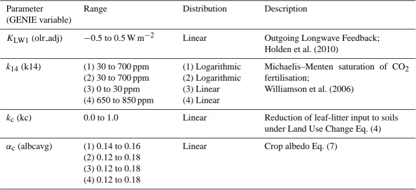
Fig. 1. 20-member ensemble-averaged 850 AD (a) vegetative carbon density and (b) soil carbon density. (c) LUC fractional change (2000– 1900 AD). (d) 20-member ensemble-averaged LUC emissions (1900 to 2000 AD, LUC forcing only, CO2relaxed to 280 ppm).

explicitly for the dynamics of natural and agricultural vege-tation. Carbon and water fluxes are linked to vegetation pat-terns and dynamics through the linkage of transpiration and photosynthesis and thus take plant water stress into account. Rising atmospheric CO2concentration affects transpiration

and biomass production through physiological and structural plant responses (Sitch et al., 2003).

Above ground biomass of the cropland area (present-day 1495 Mha) was averaged over the growing season, with sow-ing dates calculated after Waha et al. (2012). Biomass on the set aside area, represented by grass, grows between the cropping season. The time-weighted mean of crop and set-aside biomass gives the average above ground biomass es-timation of the cropland area. Managed grassland (present-day 2716 Mha) is grown over the entire year and is harvested whenever the increment of net primary production (NPP) ex-ceeds 300 gC m−2_.

4 Validation of ENTSML

The LUC implementation is validated through the applica-tion of a 20-member subset of Experiment 1, described in Joos et al. (2012). This ensemble was filtered from Exper-iment 1, applying the constraint of plausible atmospheric CO2. The subset was used in the interests of computational

efficiency, though we note that this approach does not allow us to consider the full range of modelled uncertainty. For the purposes of this validation, we apply the ensemble to a

simulation with only direct LUC forcing. In order to isolate the direct effects of LUC from the indirect effects of LUC emissions on climate and photosynthesis, atmospheric CO2

is relaxed to 280 ppm. Aspects of this experiment have been previously discussed in the inter-model comparison of Eby et al. (2012).

Figure 1a and b illustrate the ensemble-averaged spatial distributions of preindustrial (850 AD) vegetation and soil carbon density. These are provided in part to demonstrate that the ensemble distributions are similar to those obtained in tuned simulations (Lenton et al., 2006) and in part be-cause errors in carbon released by LUC can be related to er-rors in the simulation of potential vegetation and soil carbon. Deserts are less distinct than observed because atmospheric moisture transport is too diffusive. Boreal forest is generally too sparse because of insufficient moisture transport into the continental interior, and too northerly in location. Some ap-parent weaknesses of the vegetation carbon distribution in Fig. 1a (excessive forestation in the tropics and in Europe) are reconciled with modern observations through the effects of LUC (not shown). We note, however, that the excessive 850 AD forestation in Central USA is likely a result of the over-diffusive atmosphere rather than the absence of LUC at this time.

P. B. Holden et al.: A model-based constraint on CO2fertilisation 345

land–atmosphere LUC emissions from 1900 to 2000 AD. The largest fluxes are driven by removal of vegetation car-bon. However, soil emissions can be significant, especially in the Himalayas. This results from high soil densities at altitude due to lapse rate cooling, and likely too high be-cause soil weathering is not modelled. The regional dis-tributions of the LUC fluxes are generally consistent with Houghton (2008). A notable exception is the large modelled flux from central USA where, as previously noted, potential vegetation density is overstated. We do not provide a com-parison with the LUC flux distributions of Raddatz (2010) as the two approaches apply quite different assumptions. Dom-inant emissions in GENIE arise from regions associated with densely vegetated, deforested regions. Dominant emissions in Raddatz (2010) are associated with high population den-sity.

In summary, although ENTS is based around a single PFT, the climatic dependencies of this PFT are sufficient to pro-vide a reasonable spatial description of vegetative carbon density. As a result, simulated spatial patterns of LUC emis-sions also vary reasonably depending on whether the local potential vegetation is “forest” (high vegetation carbon den-sity) or “grassland” (low vegetation carbon denden-sity).

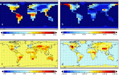
Figure 2a compares the ensemble-averaged temporal his-tory of LUC emissions with estimates of Houghton (2008) and with the LPJmL L simulation. GENIE underestimates the LUC flux, especially in recent decades. We note that this underestimate of LUC emissions is a common feature of EMICs (Eby et al., 2012). It is, however, also worth not-ing that neither the analyses of Houghton (2008) nor the LPJmL L simulation include feedbacks due to the direct cli-matic impact of LUC. These clicli-matic feedbacks (which are represented in the coupled EMICS), most notably the uptake of soil carbon driven by LUC albedo cooling, may explain part of the simulated differences. However, structural issues, most notably errors in the distributions of potential vegeta-tion, are likely to be at least as significant.

4.1 The land management parameterkc

The ensemble average in Fig. 2a conceals a substantial vari-ability in the magnitude of the simulated LUC flux. The land management parameterkc, the fractional reduction in leaf

lit-ter input to soils under LUC, is the dominant driver of LUC emission uncertainty. This is illustrated in Fig. 2b, which plots the time integrated LUC emissions (1850 to 2000) as a function ofkc. We note that very high values ofkcappear

to have been ruled out by the requirement for plausible mod-ern CO2 that was used to filter this 20-member ensemble;

the unfiltered ensemble (Experiment 1) evenly sampleskcin

the range 0 to 1. We apply the constraint of total LUC emis-sions (1850 to 2000 AD) to derive a simple calibration for

kc. Houghton (2008) emissions are 149 GTC. LPJmL

emis-sions are 181 GTC. The linear fit in Fig. 2b suggests that appropriate values ofkcare 0.45 and 0.54, respectively. We

  34  

Figure 2: a) Global LUC emissions, comparing Houghton (2008), the LPJmL_L simulation 1  

and GENIE (LUC-only forced, 20-member ensemble-average). b) Temporally integrated 2  

global LUC emissions (1850 to 2000 AD) as a function of the land management parameter kc 3  

(LUC-only forced, 20-member GENIE ensemble). 4  

5   6  

!" #" $"

#%&!" #%'!" #%(!" #(#!" #()!" #(&!" #('!" #((!"

!"#$% & '((')*$+,#$-% .$/% 0. $

*+,-./+0"$!!%" 12342"50657895":;5<:-5" =>?7="

!"#"$%$&'(")"*+&,-'" ./"#"-&,'$**" )0-" -" 0-" *--" *0-" '--" '0-" $--"

-" -&*" -&'" -&$" -&1" -&0" -&,"

!"#$% & '((')*($+,-./01///2$34#$ 56$ !" #"

  34  

Figure 2: a) Global LUC emissions, comparing Houghton (2008), the LPJmL_L simulation

1  

and GENIE (LUC-only forced, 20-member ensemble-average). b) Temporally integrated

2  

global LUC emissions (1850 to 2000 AD) as a function of the land management parameter kc

3  

(LUC-only forced, 20-member GENIE ensemble).

4  

5   6  

!" #" $"

#%&!" #%'!" #%(!" #(#!" #()!" #(&!" #('!" #((!"

!"#$% & '((')*$+,#$-% .$/% 0. $

*+,-./+0"$!!%" 12342"50657895":;5<:-5" =>?7="

!"#"$%$&'(")"*+&,-'" ./"#"-&,'$**" )0-" -" 0-" *--" *0-" '--" '0-" $--"

-" -&*" -&'" -&$" -&1" -&0" -&,"

!"#$% & '((')*($+,-./01///2$34#$ 56$ !" #"

Fig. 2. (a) Global LUC emissions, comparing Houghton (2008), the LPJmL L simulation and GENIE (LUC-only forced, 20-member ensemble-average). (b) Temporally integrated global LUC emis-sions (1850 to 2000 AD) as a function of the land management pa-rameterkc(LUC-only forced, 20-member GENIE ensemble).

apply these values as centres of two alternative priors in the Bayesian calibration ofk14 that follows. The 1-sigma width

of the priors, assumed to be Gaussian, is taken as the RMSE of the simulations with respect to the linear fit (0.11).

It is useful to discuss what uncertainty in kc is likely to

represent. By design, this parameter was intended to rep-resent the effects of land management on soil carbon. Soil carbon is reduced under cropped land because harvesting re-duces the carbon returned to the soil and because tillage in-creases soil oxidation rates. However, by applying a prior tokc that favours reasonable LUC emissions, we subsume

structural deficiencies of ENTSML into the parameterisation, such as the excessive potential vegetation in central USA or the excessive potential soil carbon at high altitude. Notably, the ENTS soil model has a single layer that reacts instanta-neously throughout its depth to surface temperature changes. Deforestation results in radiative cooling due to increased albedo, although, as has been demonstrated in more com-plex models, this is countered by decreased evaporative cool-ing, especially in the tropics (Arora and Montenegro, 2011). It is likely that an excessive decrease in soil respiration (and increase in soil carbon density) would result from the deforestation-driven cooling, i.e. the relatively high values of

346 P. B. Holden et al.: A model-based constraint on CO2fertilisation

due, at least in part, to this sensitive soil carbon response to LUC (both crop and pasture). It is important to note that our approach to calibratingkchas the effect of negating this

LUC–climate–soil carbon sink. The parameterkcis shifted

by our choice of prior to values that result in LUC emissions that are consistent with Houghton (2008), thus counteracting direct LUC–climate–carbon feedbacks. Although the pres-ence of the albedo-driven sink cannot be ruled out in nature, we prefer to assume that the sink is negligible given the sin-gle soil layer in ENTS (i.e. by applying this prior). Sensitivity to this assumption is tested by also considering a significantly lowerkc prior (centred on 0.2) in the analysis of Sect. 6.1.

This choice is influenced by previous modelling studies with tuned LUC models (Olofsson and Hickler, 2008; Stocker et al., 2011), which suggest a∼40 % reduction of leaf-litter in-put to arable soils, approximately equivalent to a global value ofkc∼0.2 when applied to all cultivated regions (ENTSML

does not distinguish between crops and pasture).

5 Methods

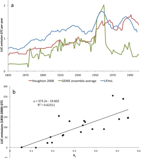
The flow chart (Fig. 3) summarises the methodology. The ensemble displayed a wide range of responses, with 671-member ensemble-averaged terrestrial carbon loss over the period 1850 to 2000 AD of 128±139 GTC (1σuncertainties are provided throughout). This compares to BernCC model estimates of∼100 to 120 GTC from the range of LUC sce-narios considered by Stocker et al. (2011), neglecting their il-lustrative scenario of a linear scaling of fractional LUC from 10 000 BC to the present. The comparison between GENIE uncertainty (∼100 GTC, driven by uncertain model param-eter values) and BernCC uncertainty (∼10 GTC, driven by alternative temporal evolutions of LUC) suggests that our ne-glect of the latter is reasonable for these purposes. We note that 123 of the 671 completed GENIE simulations exhibited an increase in terrestrial carbon storage over this period. Al-though the direct consequences of LUC can only reduce ter-restrial carbon in the model (through reductions in vegetation density and in the leaf litter-rate to soils), the effects of car-bon emissions (CO2 fertilisation and climate) and indirect

(climate-driven) LUC feedbacks, acting on both natural and cultivated vegetation, can combine to increase the modelled global terrestrial carbon reservoir.

In order to calibrate the model response, we apply the con-straint of1CO2, the simulated increase in atmospheric CO2

from 1850 to 2000 AD. This constraint is ideal for vegeta-tion calibravegeta-tion as it is associated with a negligible obser-vational error, but exhibits a wide range of simulated val-ues across the ensemble (117±41 ppm, cf. the observed in-crease of 84 ppm). It is very important to note that the ensem-ble variability is dominated by two of the poorly constrained terrestrial vegetation and land-use change parameters: 41 % of the variance in1CO2is captured by a linear dependence

on the CO2fertilisation parameterk14 and 28 % by a linear

  35  

Figure 3: Flow chart describing the experimental design.

1  

2   3  

!"#$%&%'&()*+!$,-(-%&.&(*,(&/0123.(/-4*56786*&03&%'4&********** 9:;41&0*&.*-4<)*+=#+>*

?"#$%&%'&()*+@$,-(-%&.&(*.(-03/&0.*56786*&03&%'4&*9@A=$+==A*BC>* D;2(*-11/E;0-4*,-(-%&.&(3*-11&1<* 6F,&(/%&0.3*#*.;*!**9G&HE;0*I<#)*J-'4&*#>*

6%24-.;(*;K*#@A=*.;*+===*BC*LM+*HN-0O&*PLM+*

#!)#==$%&%'&()*+@$,-(-%&.&(*&%24-.&1*&03&%'4&*;K*PLM+*

Q;3.&(/;(*1/3.(/'2E;0*K;(*LM+*K&(E4/3-E;0*,-(-%&.&(*R#!*9D/O2(&*?>*

6%24-.&*&03&%'4&*;2.,2.*;K*PLM+*-3*-*

I(1_{*;(1&(*,;4S0;%/-4*K20HE;0*;K*.N&*+@*}

/0,2.*,-(-%&.&(3*9T8L*.&(%*3&4&HE;0>*

T-S&3/-0*H-4/'(-E;0*96U*">* T-3&*H-3&V*

,9W/X>*Y*Z9RH)*=<!A)*=<##>)*[\*Y*=,,%)*]\*Y*#",,%*

^-01;%*H;%'/0-E;03*;K*!*.(-03/&0.* ,-(-%&.&(3*9J-'4&*#>*-11&1*.;*.N&*!"=* H;%,4&.&1*,4-23/'4&*,-(-%&.&(*3&.3* 9&-HN*I=*E%&3>*-3*/0,2.*.;*&%24-.;(*

T/00&1*&%24-.&1*PLM+*1-.-*9#=F#=*1-.-*'/03V*H(;,*%-0-O&%&0.*

,-(-%&.&(*RH*-01*LM+*K&(E4/3-E;0*,-(-%&.&(*R#!>*

Fig. 3. Flow chart describing the experimental design.

dependence on the land management parameterkc. The

en-semble variability due to all other 26 parameters together generate an uncertainty of∼16 ppm, compared tok14andkc,

which together contribute∼38 ppm. For this reason, we only consider the calibration of these two parameters. To further illustrate, the dominant correlations between parameters and

1CO2 are CO2 fertilisationk14: −0.64; crop management

parameterkc: 0.53; ocean wind-stress scaling WSF:−0.16;

soil respiration temperature dependence SRT: 0.15; and crop albedoαc:−0.15. WSF is the dominant parameter driving

uncertainty of ocean uptake (Holden et al., 2012). The weak correlation with SRT may be partly explained through the two opposing drivers of changing soil respiration – global CO2-driven warming and local LUC-driven cooling. Given

the dominant controls exerted byk14 andkc, the remaining

26 parameters are not well constrained by1CO2, although

we note that, in general, they have already been constrained by the requirement for preindustrial plausibility. It should also be emphasised, however, that these 26 parameters do contribute to significant uncertainty across the ensemble that, together with inherent structural error, limit the degree to which CO2fertilisation can be constrained.

We choose to constrain on the basis of1CO2rather than

present-day CO2 as we are here concerned with the

re-sponse of the system to changing CO2 and this approach

avoids additional uncertainty due to an imperfect prediction of the preindustrial state. We prefer to avoid the alterna-tive approach of tightly constraining by preindustrial CO2

P. B. Holden et al.: A model-based constraint on CO2fertilisation 347

which is to rule out only those simulations which are un-controversially implausible, necessary (Edwards et al., 2011) for the Bayesian calibration which follows. We note that ensemble-averaged preindustrial CO2(280±15 ppm) is well

centred on observations. The variability can be largely at-tributed to∼centennial-scale instabilities that are apparent in

∼30 % of the simulations that appear to be related to the pres-ence of alternative stable states, likely driven by ocean con-vection and/or stratification-dependent mixing. We choose not to filter out these simulations, in part as it was found to be very difficult to distinguish the instability from natural variability with an objective test. Imposing (somewhat sub-jective) tests to eliminate simulations that display an instabil-ity was not found to have a significant effect on the emula-tion and calibraemula-tion that follows, but including all simulaemula-tions provides a weaker but more reliable constraint as it captures the complete range of ensemble variability.

It is not appropriate to derive marginal probability distri-butions for the two parameters without first considering their joint probability distribution, especially given the strong de-pendencies of1CO2on both of these parameters which leads

to strong correlations between the parameters in plausible pa-rameter space. The 671 completed simulations are not suf-ficient to sample the 28-dimensional input space to prop-erly quantify either the expectation or the parametric uncer-tainty throughout the 2D subspace of CO2 fertilisation and

land management. We note that the parametric uncertainty of1CO2within the 2-D subspace (i.e. arising from the other

26 parameters) is not constant, ranging from 14 ppm (lowkc,

highk14)to 24 ppm (highkc, lowk14). In order to generate

sufficient data to adequately sample the 28-dimensional in-put space, we first build an emulator of1CO2, building on

Edwards et al. (2011) who used an emulator to identify im-plausible regions of input parameter space. This emulator is needed to fully and evenly sample the 28-dimensional input space in order to provide well-quantified estimates of both expectation and uncertainty at all points in thek14/ kc

sub-space.

We take the 28 parameters as emulator inputs and con-struct a cubic emulator following a similar procedure to that described in Holden et al. (2010). Our emulator attempts to fit the simulated values of1CO2to a polynomial function of the

input parameters. A quadratic emulator was first built, allow-ing cross terms between all 28 parameters, to which we allow the addition of cubic terms before applying the Bayes infor-mation criterion (BIC) to reduce the model size. The addi-tional cubic terms considered were the four cubic terms that were generated by an investigative emulation that allowed all possible cubic terms but considered only the 16 significant parameters in the quadratic model. This approach was taken to improve the efficiency of the process relative to an ap-proach that considers all possible cubic terms from 28 model parameters. Two cubic terms were retained after application of BIC (k3₁₄ and κT ×k142, where κT is atmospheric heat

diffusivity). The resulting emulator fits the simulated data well, with anR2of 94 %.

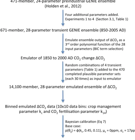
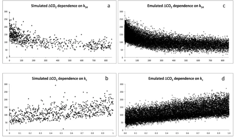
We then designed a 14 100-member parameter set to apply as input to this emulator. The design reproduces 470 of the 471 simulated parameter sets (omitting a single parameter set which did not complete in Experiment 2) thirty times, replac-ing the four transient parameters with a 4×14 100 matrix of randomly generated inputs across the ranges in Table 1. The output of this emulated ensemble is compared with the sim-ulated ensemble in Fig. 4, illustrated by the marginal depen-dencies onk14 andkc. The response to changes in these

pa-rameters is well captured by the emulator. Although the most extreme values of1CO2are underestimated by the smooth

polynomial functions, the emulated ensemble distribution of 115±39 ppm compares favourably to the simulated distribu-tion (117±41 ppm), suggesting this reduction in variance is unlikely to be significant. It is worth noting that the simulator cannot reproduce observed1CO2(84 ppm) with low values

ofk141.

To derive a joint probability distribution we first gener-ate a two-dimensional matrix of data bins. We subdivide the

kc/ k14 parameter space into 10×10 bins, linearly spaced

forkc(i=1,10) and quadratically spaced fork14(j=1,10),

across the ranges of their prior distributions (Table 1). Within each of the 10×10 bins we calculate the meanµij and

stan-dard deviationσij of simulated1CO2. Within each bin the

variance is dominated by uncertainty due to the remaining 26 ensemble parameters as, to first order, k14 and kc are

fixed. We apply Bayes’ theorem to the bin statistics to de-rive a posterior distribution for each bin. Analogously to Rougier (2007), we apply

p θij|1CO2=

cϕ1CO2, µij+µε,

q

σ_ij2+σ2

ε

p θij, (8)

where ϕ describes a normal distribution, evaluated at

1CO2=84 ppm with meanµij+µεand standard deviation

√

(σ_ij2+σ_ε2),µεandσε are model structural bias and

struc-tural error, respectively,cis a normalising constant, θij are

the binned values of thek14/ kcparameter pair, andp(θij)the

prior probability we assign to that combination. In this ap-plication, the resulting pdf was found to give similar results to a more rigorous calibration procedure that explicitly inte-grated over the individual outputs of the emulated ensemble (i.e. rather than approximating emulator output with a binned normal distribution).

It is essential to include estimates of structural error and bias in a model calibration to avoid over-constraining the re-sulting pdf. We derive an estimate for structural error by ap-plying an approach influenced by Murphy et al. (2007) who suggest the inter-model spread of a quantity can be used to provide a measure of structural error, reflecting, at least in

1_{Neglecting the single simulation that entered a Snowball Earth}

348 P. B. Holden et al.: A model-based constraint on CO2fertilisation

Fig. 4. Simulated CO2dependence on (a) CO2 fertilisation parameterk14 and (b) land management parameter kc, compared with the emulated CO₂dependencies on (c)k14and (d)kc.

part, different structural choices that can be made. Although such an approach is likely to provide an underestimate be-cause different models likely share some sources of struc-tural error, it is conservative in the sense that a component of the inter-model variability will arise from parametric un-certainty (but be attributed to structural error). C4MIP sim-ulations forced by SRES A2 exhibit a standard deviation of

∼90 ppm in the simulated increase in CO2 in 2100 relative

to 2000 (Friedlingstein et al., 2006). We note that Friedling-stein et al. (2006) found no systematic differences between the behaviours of OAGCMs and EMICs. We obtain an esti-mate of structural error by linearly scaling the C4MIP inter-model variability by the relative increase in CO2, i.e. by 1CO2/480 ppm, where 480 ppm is the C4MIP intermodel

average increase (2000 to 2100). This gives a1CO2

struc-tural error of±17 ppm. The ensemble relationship between

1CO2and total emissionsT (the sum of time integrated

fos-sil fuel and net terrestrial carbon emissions) is well described (R2=91 %) by

1CO2=0.2889T . (9)

This relationship suggests that the assumed structural er-ror in1CO2is equivalent to a 2-sigma uncertainty in

accu-mulated historical emissions of∼120 GTC, sufficient to en-compass uncertainties in historical fossil fuel emissions (cf. accumulated emissions of∼280 GTC).

In our LUC implementation, a potentially significant source of structural bias is the assumption that vegetative carbon is negligible in cultivated regions, leading to ex-cess simulated LUC emissions. The LPJmL LCC simulation

quantifies this neglect, yielding a global above-ground LUC biomass of 3 GTC, equivalent to an over-estimation of1CO2

by∼1 ppm which can reasonably be neglected in the calibra-tion.

6 Results

6.1 Calibration of CO2fertilisation parameter

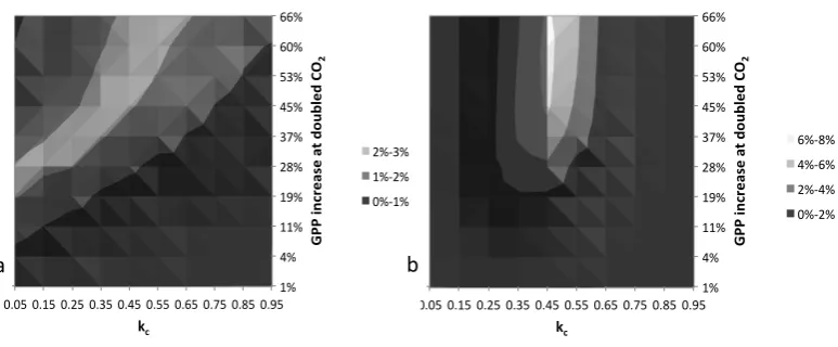
We apply Eq. (8) to derive the joint probability distribution forkc (land management) andk14 (CO2fertilisation),

illus-trated in Fig. 5. In these plots,k14is re-expressed as the

per-centage increase in photosynthesis in response to a doubling of CO2from preindustrial levels in order to facilitate

compar-ison with alternative estimates. Figure 5a applies a uniform prior; Fig. 5b constrains the loss in cultivated soil carbon to more reasonable values by applying thekc prior centred on

0.45 (Sect. 4). In both plots, structural error ofσε=17 ppm

and structural biasµε=0 ppm are applied (Sect. 5). We

in-tegrate over the joint distribution in Fig. 5b to derive the marginal probability distribution fork14, plotted as the blue

curve in Fig. 6a and b. This analysis demonstrates a GPP increase in response to doubled CO2that is most likely 40–

60 %, and very likely (90 % confidence) to exceed 20 %. Note that high values ofk14 are not well constrained by the pdf.

This is in part due to the low sensitivity of the saturating Michaelis–Menten function at high values ofk14, although

P. B. Holden et al.: A model-based constraint on CO2fertilisation 349

37  

Figure 5

: Joint probability distributions for land management parameter k

and CO

1  

fertilisation parameter k

, applying Eq. 8 with a) a uniform prior distribution p(

θ

) = 1 and b)

2  

a prior assumption for k

, p(

θ

) =

φ

(k

, 0.45, 0.11). Note that k

is re-expressed as the

3  

percentage increase in GPP in response to a doubling of CO

from preindustrial levels.

4  

5  

6  

!"# $"# !!"# !%"# &'"# ()"# $*"# *("# +,"# ++"#

,-,*# ,-!*# ,-&*# ,-(*# ,-$*# ,-**# ,-+*# ,-)*# ,-'*# ,-%*#

!""#$ %&'() *(#) +#, -. /0 (, #12 3# 4_&# +".'"# $".+"# &".$"# ,".&"# !"# $"# !!"# !%"# &'"# ()"# $*"# *("# +,"# ++"#

,-,*# ,-!*# ,-&*# ,-(*# ,-$*# ,-**# ,-+*# ,-)*# ,-'*# ,-%*#

!""#$ %&'() *(#) +#, -. /0 (, #12 3# 4&# &".("# !".&"# ,".!"#

!"

#"

Fig. 5. Joint probability distributions for land management parameterkcand CO2fertilisation parameterk14, applying Eq. (8) with (a) a uniform prior distributionp(θij)=1 and (b) a prior assumption forkc,p(θij)=ϕ(kc, 0.45, 0.11). Note thatk14 is re-expressed as the percentage increase in GPP in response to a doubling of CO₂from preindustrial levels.

38  

Figure 6: Sensitivity analysis of the marginal probability distribution for the GPP increase in

1  

response to a doubling of CO

to a) the land management parameter k

prior assumption and

2  

b) the structural error assumed for the simulation of

Δ

CO

.

3  

4  

5  

!"!# !"$# !"%#

!# !"$# !"%# !"&# !"'# !"(# !")# !"*#

!"# $% $& '&( )* +!!*&,-".%/.*%(*0#1$'.0*234* 5.,/&67&()*(#*!"&#"* +,-.# /0#12302# !"%#45#12302# !"('#12302# !" !#$" !#%"

!" !#$" !#%" !#&" !#'" !#(" !#)" !#*"

!""#$%&'()*(#)+#,-./0(,#123# 4(%*5675+8#+-#4+'.&+.')0#9''-'# +,-." /0"12" !#'("34"567068"&#%559":7,-" !#%"34"567068"%%#)559":7,-"

Figure 6

: Sensitivity analysis of the marginal probability distribution for the GPP increase in

1  

response to a doubling of CO

to a) the land management parameter k

prior assumption and

2  

b) the structural error assumed for the simulation of ΔCO

.

3  

4  

5  

!"!# !"$# !"%#

!# !"$# !"%# !"&# !"'# !"(# !")# !"*#

!"# $% $& '&( )* +!!*&,-".%/.*%(*0#1$'.0*234* 5.,/&67&()*(#*!"&#"* +,-.# /0#12302# !"%#45#12302# !"('#12302# !" !#$" !#%"

!" !#$" !#%" !#&" !#'" !#(" !#)" !#*"

!""#$%&'()*(#)+#,-./0(,#123# 4(%*5675+8#+-#4+'.&+.')0#9''-'# +,-." /0"12" !#'("34"567068"&#%559":7,-" !#%"34"567068"%%#)559":7,-" (a) (b)

Fig. 6. Sensitivity analysis of the marginal probability distribution for the GPP increase in response to a doubling of CO2to (a) the land management parameterkcprior assumption and (b) the structural error assumed for the simulation of1CO2.

sufficient to quantify a lower bound fork14(90 % confidence)

and to identify the approximate range of most likely values. Figure 6a illustrates sensitivity to the assumed prior distri-bution for land managementkc. The base casekcprior (mean

0.45, standard deviation 0.11) constrains CO2 fertilisation

with temporally integrated LUC emissions of 149 GTC (Houghton, 2008) as described in Sect. 4.1. The sensitivity experiment withkccentred on 0.54 was constrained with the

higher LUC emissions of the LPJmL simulation (181 GTC), and requires a slightly stronger CO2fertilisation effect to

bal-ance the carbon budget. i.e. to match observed1CO2. The

sensitivity experiment withkccentred on 0.2 is equivalent to

a constraint based on LUC emissions of 55 GTC. This as-sumption is equivalent to an LUC-climate feedback sink (the effect of LUC-driven albedo changes on soil respiration) of

∼90 GTC. The additional sink implicit in this analysis shifts

the most likely CO2fertilisation effect (in response to

dou-bled CO2)to∼30 %. A further sensitivity experiment applies

a uniform prior and produces a similar, though somewhat broader, pdf to the base case. This similarity does not sug-gest that the calibration is insensitive to the prior, but rather it reflects the fact that the base case prior is approximately centred on the ensemble distribution ofkc.

Figure 6b illustrates sensitivity to the structural error as-sumption. Two analyses are performed to investigate the structural bias term. The first of these has akcprior centred

on 0.45 and a structural bias ofµε=3.2 ppm. This bias is

included for the underestimate of LUC emissions (converted to1CO2 with Eq. 9) compared to Houghton (2008) when

this prior is applied to the 20-member ensemble (Sect. 4.1). The second sensitivity analysis has akcprior centred on 0.2

and a structural bias ofµε=22.6 ppm. This is an alternative

350 P. B. Holden et al.: A model-based constraint on CO2fertilisation

approach to the calibration: we assume that thekc=0.2 prior

is reasonable, but instead correct for the low LUC emissions relative to Houghton (2008) through the structural bias term. These two analyses produce similar pdfs. A further illustra-tive analysis applies no structural error (σε=0 ppm). This

calculation imposes a stronger constraint on k14, but one

which cannot be justified as it is equivalent to assuming that the only model uncertainty is due to uncertainty in the input parameters.

The base case pdf fork14is generally robust with respect

to these various sensitivities, with the exception of the choice ofkcprior. The dependency onkcis unsurprising given that

both parameters are comparably important in determining

1CO2, necessitating the analysis of the joint probability

dis-tribution. As previously noted, the calibration does not quan-tify the upper bound for CO2fertilisation. The most likely

GPP response to a doubling of CO2is 40–60 %, equivalent to

ak14range of∼300–600 ppm (and consistent with the

simu-lated ranges most likely to produce plausible CO2plotted in

Fig. 4a). We note that these values fork14 are significantly

greater than in the standard ENTS value (Williamson et al., 2006, 145 ppm equivalent to a 24 % increase in GPP under doubled CO2).

6.2 Calibrated ensemble output

We apply the parameter calibrations to weigh individual simulated ensemble members in order to derive calibrated model outputs of global GPP (2000 AD), post-industrial ter-restrial carbon change (1850 to 2000), land–atmosphere car-bon flux (1990–2000 average) and ocean–atmosphere carcar-bon flux (1990–2000 average). Each of these quantities is of im-portance to the global carbon cycle and each is associated with significant uncertainty. These analyses were performed in part to provide independent estimates of these widely stud-ied metrics, and in part as a validation of the calibration.

We consider the 470 completed simulations that comprise Experiments 1 and 2. We do not include Experiments 3 and 4, as these simulations were performed to better quantify the simulated response at the tails of thek14 distribution. Their

inclusion would compromise the prior distribution ofk14by

attributing too much weight to the tails.

The temporal evolution of atmospheric CO2is plotted in

Fig. 7. The ensemble-averaged distribution overstates the rise in CO2, unsurprising given that the calibration of Sect. 6.1

suggests that the ensemble-averaged value ofk14 (212 ppm,

equivalent to a 32 % GPP increase under doubled CO2)is too

low to match the observed change in atmospheric CO2. The

calibrated curve is better matched, although it underestimates atmospheric CO2by up to∼10 ppm between 1850 and 1950

(and overestimates1CO2). The sharp drop in CO2at 1815

is associated with the Tambora volcanic eruption and reflects the unreasonably fast response time of the single-layer soil pool to surface cooling (see Sect. 4.1). However, the com-parably rapid recovery suggests that this sink is unlikely to

  39  

Figure 7: The temporal evolution of atmospheric CO2.

1  

2   3   4  

!"#$%&'( !")$%&'( !"*$%&'( +",$%&'( +"+$%&'( +"#$%&'( +")$%&'( +"*$%&'( '",$%&'(

,)#&( ,-&&( ,-#&( ,*&&( ,*#&( !&&&(

!"#

$%&

&'(

$

./012345670( $7018/91(43124:1( ;49</24=1>(17018/91(

Fig. 7. The temporal evolution of atmospheric CO2.

explain the low CO2estimates that persist through to 1950.

A more likely explanation is the underestimate of early LUC emissions (Fig. 2a).

The following discussion considers a series of posterior pdfs (Fig. 8). In order to generate these pdfs, we subdivided the output space into data bins and summed the probability weights of all simulations that fall into each bin. The width of the bins was chosen to remove fine structure from the pdf. We assume that this fine structure is unlikely to be physi-cally meaningful. The binning approach is crudely equivalent to ascribing a structural error to each model output, rather than accepting it as a point estimate. Each figure illustrates the calibrated GENIE pdf, together with the 66 % confidence interval, and the point estimates from the LPJmL LCC and LPJmL LC simulations, respectively, including and neglect-ing the direct effect of CO2on vegetation.

Figure 8a plots the pdf of global natural GPP (2000 AD). ENTSML does not calculate GPP in cultivated regions but applies the simplifying assumption of instantaneous harvest-ing and grazharvest-ing. The GENIE calibration (likely in the range 107 to 152 GTC yr−1) is therefore limited to global GPP in regions unaffected by LUC. The LPJmL LCC simula-tion quantifies this neglect to be ∼7 GTC yr−1 (crops) and

∼29 GTC yr−1(pasture). The LPJmL LCC estimate of nat-ural GPP of∼97 GTC yr−1(1991 to 2000 average) is some-what lower than the GENIE pdf, although consistent with the 2-sigma uncertainty. A recent observational based esti-mate of global GPP (Beer et al., 2010) is 123±8 GTC yr−1_,

of which 15 GTC yr−1_{was attributed to croplands. It is}

im-portant to note that the GENIE calibration of GPP is not well constrained by1CO2(which rather constrains the

P. B. Holden et al.: A model-based constraint on CO2fertilisation 351

  40  

Figure 8: Probability distributions of carbon exchange between land-atmosphere-ocean. Each

1  

calculation applies the base case prior distribution for the land management parameter kc, 2  

p(θij) = φ(kc, 0.45, 0.11), together with the posterior distribution for CO2 fertilisation 3  

parameter k14 (base case, Fig 6) to probability weight each of the 470 completed GENIE 4  

simulations (Experiments 1 and 2). Distributions are a) global GPP (2000), b) change in

5  

terrestrial carbon over the post-industrial period (1850 to 2000), c) annually-averaged

land-to-6  

atmosphere flux (1990 to 2000) and d) annually-averaged ocean-to-atmosphere flux (1990 to

7  

2000). Vertical dashed lines illustrate the 66% confidence interval. In a-c, the dark green

8  

vertical bar is the LPJmL_LCC simulation (including the direct CO2 effect) and the light 9  

green vertical bar is the LPJmL_LC simulation (neglecting the direct CO2 effect). 10  

11  

12  

!"!#$ !"%#$ &"!#$ &"%#$ '"!#$ '"%#$

%!$ (!$ &&!$ &)!$ &*!$ '!!$

!"#

$%

$&

'&(

)*

+,,,*-'#$%'*.%(/"%'*-!!*0-123*

!"!#$ !"%#$ !"&#$ !"'#$ !"(#$

)&!!$ )*!!$ )%!!$ )+!!$ !$ +!!$ %!!$ *!!$ &!!$

!"#

$%

$&

'&(

)*

+#(%'*,-%./0*&.*(0""01("&%'*,%"$#.*23456786669*2:+;9*

!"# $!"# %!"# &!"# '!"# (!"#

)(# )&# )$# $# &# (#

!"#

$%

$&

'&(

)*

+,-"%.-*'%/01%(2#345-"-*678*9:;;<1=<<<>*9?@A)"1:_>*

!"# $!"# %!"# &!"# '!"# (!!"#

)*# )+# )(# (# +# *#

!"#

$%

$&

'&(

)*

+,-"%.-*'%/01#2-%/*345*678891:999;**6<=>)"17_;*

!" #"

$" %"

Fig. 8. Probability distributions of carbon exchange between land–atmosphere–ocean. Each calculation applies the base case prior distribution for the land management parameterkc,p(θij)=ϕ(kc, 0.45, 0.11), together with the posterior distribution for CO2fertilisation parameterk14 (base case, Fig. 6) to probability weight each of the 470 completed GENIE simulations (Experiments 1 and 2). Distributions are (a) global GPP (2000), (b) change in terrestrial carbon over the post-industrial period (1850 to 2000), (c) annually averaged land–atmosphere flux (1990 to 2000) and (d) annually averaged ocean–atmosphere flux (1990 to 2000). Vertical dashed lines illustrate the 66 % confidence interval. In (a)–(c), the dark green vertical bar is the LPJmL LCC simulation (including the direct CO2effect) and the light green vertical bar is the LPJmL LC simulation (neglecting the direct CO2effect).

moisture diffusivity (R2=44 %), soil respiration tempera-ture dependence (16 %), baseline photosynthesis rate (13 %), atmospheric heat diffusivity (10 %), baseline leaf litter rate (10 %) and, finally, the CO2fertilisation parameterk14(6 %).

Global GPP in LPJmL (natural and cultivated) increases by 9.3 % due to the direct effect of a 22 % increase in CO2

(i.e. between 1900 and 2000 AD). This compares to the GE-NIE calibration (Sect. 6.1) in response to a doubling of CO2

of a most likely increase of 40–60 %, very likely to be more than 20 %.

Figure 8b plots the posterior distribution of post-industrial terrestrial carbon change (2000–1850). This analysis pre-dicts a 66 % probability that the change in terrestrial biomass lies between a loss of 0 and 128 GTC. The probability-weighted mean of 66 GTC provides a best estimate of net post-industrial land emissions, consistent with data-driven estimates (for the period 1800 to 1994) of 39±28 GTC (Sabine et al., 2004). We note that the linear fit of Eq. (9) esti-mates most likely historical net land emissions to be 13 GTC. The higher terrestrial carbon losses in the probabilistic cali-bration likely reflect the ensemble prior distribution fork14,

which favours a weaker land sink, being logarithmically spaced from 30 to 700 ppm (cf. the calibrated estimate of

∼300 to 600 ppm). The LPJmL LCC result (including CO2

fertilisation) lies within the calibrated pdf. The LPJmL LC

result (neglecting CO2fertilisation) does not. This suggests

that plausible post-industrial net land emissions can only be simulated in LPJmL (at default parameters) if the direct ef-fect of CO2is included.

Figure 8c illustrates calibrated pdf of the land–atmosphere carbon flux over the recent period (1990 to 2000 average). This has a probability-weighted mean of−0.7 GTC yr−1and a 66 % confidence interval of uncertain sign, ranging from

−1.7 to 0.4 GTC yr−1. LPJmL can only simulate a plausi-ble land–atmosphere flux under the assumption of a direct CO2effect. The GENIE estimates compare with IPCC

esti-mates (Denman et al., 2007) of−1.0±0.6 GTC yr−1. More recently, Le Qu´er´e et al. (2009) estimated LUC emissions (1990 to 2005) of 1.5±0.7 GTC yr−1 _{offset by a}

terres-trial sink (1990 to 2000) of 2.6±0.7 GTC yr−1_{, implying}

a net land–atmosphere flux of−1.1±1.0 GTC yr−1_{. Joos et}

al. (1999) applied the single deconvolution approach, closely related to the approach taken here as both use an ocean model to constrain carbon uptake and solve for the resid-ual land–atmosphere flux, to estimate the 1990 flux to be

−0.8 GTC yr−1.