Daniel B. Tait
Thesis submitted to the Faculty of the Virginia Polytechnic Institute and State University in partial fulfillment of the requirements for the degree of
Master of Science in
Electrical Engineering
R. Michael Buehrer, Chair Harpreet S. Dhillon Steven W. Ellingson
August 12, 2020 Blacksburg, Virginia
Keywords: Direction-of-Arrival Estimation, Array Signal Processing, ESPRIT, Independent Component Analysis, Cyclostationarity, Higher-Order Statistics
Daniel B. Tait (ABSTRACT)
Daniel B. Tait
(GENERAL AUDIENCE ABSTRACT)
List of Figures vii
List of Tables x
1 Introduction 1
1.1 Motivation. . . 2
1.2 Prior Work . . . 5
1.3 Contributions . . . 8
1.4 Outline . . . 8
2 Background 10 2.1 Modeling . . . 11
2.1.1 Electromagnetic Vector-Sensor Model . . . 11
2.1.2 Signal Model . . . 16
2.2 Direction-of-Arrival Estimation with Subspace Techniques . . . 18
2.2.1 Uni-Vector-Sensor ESPRIT Algorithm . . . 20
2.3 Performance Metrics . . . 25
2.4 Cyclostationarity . . . 27
2.5 Higher-Order Statistics . . . 29
3.2 Cyclostationarity-based UVS-ESPRIT . . . 37
3.3 Cumulant-based UVS-ESPRIT . . . 43
3.4 Electromagnetic Vector-Sensor Observability . . . 50
4 Results and Discussion 52 4.1 Simulation Setup . . . 53
4.2 Algorithm Performance . . . 57
4.2.1 Performance without Interference . . . 57
4.2.2 Performance with Interference . . . 70
4.2.3 Discussion . . . 73
4.3 The Spectral Overlap Problem. . . 74
4.3.1 Results . . . 74
4.3.2 Discussion . . . 80
4.4 Additional Results . . . 81
4.4.1 Time-Lag for Non-Deterministic Sources . . . 81
4.4.2 Spatial Diversity and Observability . . . 83
4.4.3 Estimating More Sources Than Sensor Elements . . . 84
4.5 Algorithm Comparison . . . 87
5.2 Future Work . . . 89
Bibliography 91
Appendices 100
Appendix A Independent Component Analysis for DOA Estimation 101
Appendix B Simulation Conditions 106
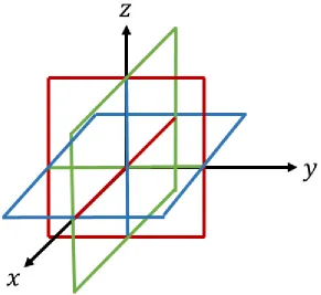
2.1 Visual representation of a single electromagnetic vector-sensor, comprised of both dipole and magnetic loop antennas. The x-oriented elements are shown
in red, they-oriented elements are shown in green, and thez-oriented elements
are shown in blue. . . 13
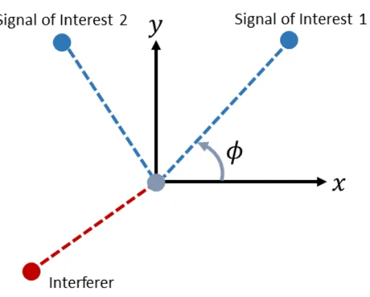
2.2 Visual representation of the problem with three sources present. In this case, the DOA of the two signals-of-interest would be estimated, while the interferer would be neglected. All sensor elements are located at the origin. . . 15
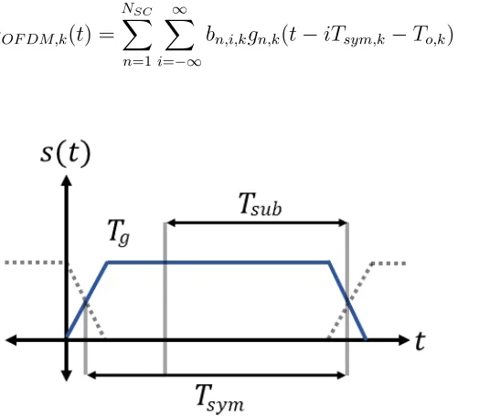
2.3 Time-domain representation showing the windowing and guard interval of an OFDM subcarrier. . . 17
3.1 Cylic correlogram for a PAM digital signal with raised-cosine pulse shaping and Tsym= 16 samples.. . . 40
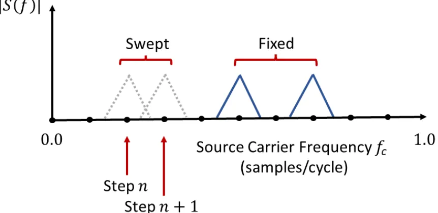
4.1 Visual representation of how the frequency sweep is performed when three sources are present. This depicts the power spectrum for a single channel, whereas the the electromagnetic vector-sensor contains six. . . 56
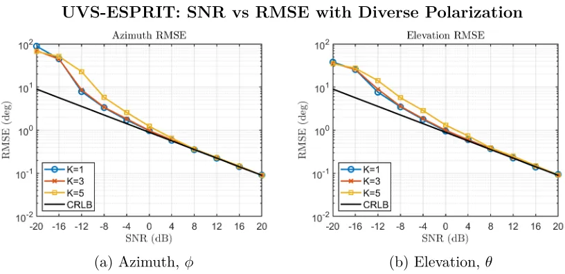
4.2 UVS-ESPRIT RMSE for up to five diversely polarized harmonic sources. . . 58
4.3 UVS-ESPRIT RMSE for up to five linearly polarized harmonic sources. . . . 58
4.4 UVS-ESPRIT RMSE for up to five diversely polarized PAM digital sources with Tsym = 64. . . 60
4.6 UVS-ESPRIT RMSE for up to five diversely polarized OFDM digital sources with Tsym = 64. . . 62
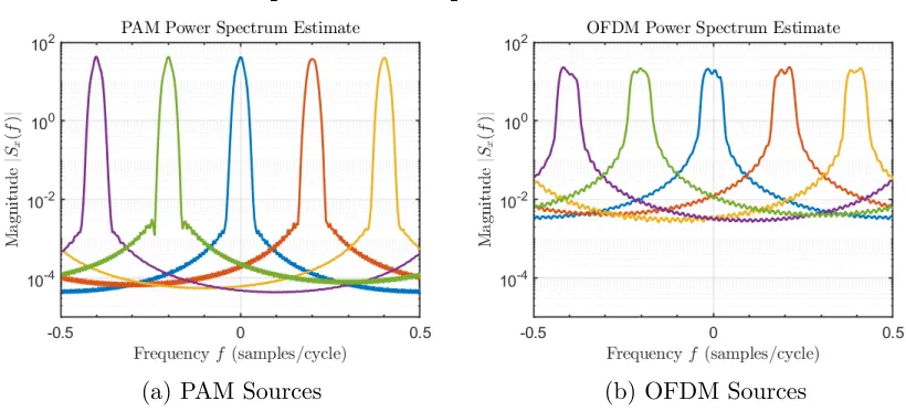
4.7 Comparison between the PAM and OFDM power spectra. . . 62
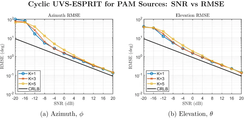
4.8 Cyclic UVS-ESPRIT RMSE for up to five diversely polarized PAM digital sources with Tsym = 64 and α= 1/Tsym. . . 64
4.9 Cylic correlogram for a OFDM digital signal. . . 65
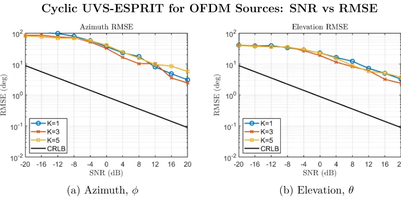
4.10 Cyclic UVS-ESPRIT RMSE for up to five diversely polarized OFDM digital sources with Nsc = 10, Tsym = 256, and Tg =Tsym/4. . . 66
4.11 Cumulant UVS-ESPRIT RMSE for up to five diversely polarized PAM digital sources with Tsym = 64 and square pulse-shaping. . . 67
4.12 Performance of Cumulant UVS-ESPRIT with variable kurtosis due to differ-ent waveforms. . . 69
4.13 Performance of cumulant ESPRIT with variable kurtosis due to the digital constellations. . . 69
4.14 Performance of the Cyclic UVS-ESPRIT algorithm when an interferer is present. 71
4.15 Performance of the Cumulant UVS-ESPRIT algorithm when an interferer is present. . . 72
4.16 Performance of the UVS-ESPRIT algorithm when there is spectral overlap for two sources. . . 75
4.18 Performance of the Cyclic UVS-ESPRIT algorithm when there is spectral overlap for two sources with the same cycle frequency.. . . 78
4.19 Performance of the Cumulant UVS-ESPRIT algorithm when there is spectral overlap for two sources, where fk ∈ {0.20,0.30}. . . 79 4.20 RMSE of the UVS-ESPRIT algorithm for harmonic and digitally modulated
sources as the time lag increases, where fc ∈ {0.0,0.5}. . . 82 4.21 Estimates for fixed azimuth and elevation forK = 16sources andT = 32trials. 83
4.22 Example trials where φ∼Unif[0◦,360◦] and θ ∼Unif[45◦,135◦]. . . 84 4.23 Cumulant UVS-ESPRIT algorithm for a large number of sources and variable
frequency spacing. . . 86
A.1 JADE RMSE for up to five diversely polarized PAM digital sources. . . 104
A.2 JADE estimating the DOA of more sources than sensor elements for various SNR. . . 105
4.1 Comparison of the algorithms discussed in this thesis. . . 87
B.1 Simulations for UVS-ESPRIT without interference. . . 106
B.2 Simulations for Cyclic/Cumulant UVS-ESPRIT and the JADE algorithm without interference. . . 107
B.3 Simulations for Cyclic/Cumulant UVS-ESPRIT with interference. . . 108
B.4 Simulations for UVS-ESPRIT with spectral overlap.. . . 108
AWGN Additive White Gaussian Noise
CRLB Cramer-Rao Lower Bound
DOA Direction-of-Arrival
EMVS Electromagnetic Vector-Sensor
ESPRIT Estimation of Signal Parameters via Rotational Invariant Techniques
JADE Joint Approximate Diagonalization of Eigenmatrices
MUSIC MUltiple SIgnal Classification
OFDM Orthogonal Frequency Division Multiplexing
PAM Pulse Amplitude Modulation
QAM Quadrature Amplitude Modulation
QPSK Quadrature Phase-Shift Keying
RMSE Root-Mean-Squared Error
SIR Signal-to-Interference Ratio
SNOI Signal-Not-of-Interest
SNR Signal-to-Noise Ratio
SOI Signal-of-Interest
UVS Uni-Vector-Sensor
Introduction
This chapter first discusses the motivation behind the investigation into signal processing for a single electromagnetic vector-sensor and the relevance of DOA estimation. The general motivation behind conducting research into this subject is discussed and an explanation is provided into why additional algorithms based on cyclostationarity and higher-order statis-tics are investigated for estimating the DOA in the presence of interference.
After presenting the motivations, the prior contributions which form the basis of this work are provided to the reader. This includes a general discussion on DOA estimation and its relation to cyclostationary signal processing and higher-order statistics for array signal processing applications. Valuable references are provided to the reader that, so those who are interested in further exploration of this topic will know where to begin.
Finally, the distinctive contributions of this thesis to the DOA estimation problem for a single electromagnetic vector-sensor are presented and the content of each chapter is outlined.
1.1 Motivation
The direction-of-arrival estimation problem is related to the localization problem where the angular-spatial parameters of one or more wavefronts (also referred to as sources) impinging upon an array of sensors is estimated. The design of these sensors and the implementation of the DOA estimation algorithms in these systems can vary depending on the topology of the array because of the mapping between the wavefront and the array. For example, the approach taken towards applying DOA estimation algorithms to a uniform linear array of dipoles differs from those applied to a circular array [35]. In general, there are three classes of algorithms that may be applied to these sensor arrays: classical beamforming algorithms, parametric methods, and high-resolution subspace algorithms [55, 58]. The focus in this thesis is on a derivative of the high-resolution subspace algorithm ESPRIT for a single electromagnetic vector-sensor, termed Uni-Vector-Sensor ESPRIT by Wong and Zoltowski [61], and its application in the presence of interference.
One such sensor applicable to the DOA estimation problem is the electromagnetic vector-sensor. These sensors are comprised of three orthogonally oriented dipoles and three orthog-onally oriented magnetic loops. The orthogonal orientation of the sensor elements provides the capability of capturing the full electric and magnetic field vectors at a point in space from the impinging wavefronts, which enables the sensor to uniquely estimate the DOA through the Poynting vector of its array manifold vectors [39]. In general, algorithms typically rely on interferometric approaches for spatially displaced elements, but the vector-sensor may have advantages over arrays with displaced dipoles. Chevalier suggests arrays with co-located elements may estimate the DOA of more sources than spatially displaced arrays [11].
breadth of applications in the modern world and the insatiable demand for higher perfor-mance and reduced complexity. The DOA estimation problem has found applications in a range of areas including wireless communications, radar, sonar, electronic warfare, and more [58]. There are civilian applications for DOA estimation, such as cognitive radio and its role in beamforming, as well as military applications. In some cases, these problems call for capabilities that selectively estimate the DOA of a signal-of-interest (SOI) through its statistical properties in the presence of interference.
Several algorithms have been devised that are applicable to a single electromagnetic vector-sensor. One example is the cross product estimator by Nehorai [39], although this approach can only reliably estimate the DOA of a single source in the absence of interference and has lower-resolution than ESPRIT-based subspace algorithms. Another approach is to compare the array manifold to a library of vectors through a search algorithm, but this requires a computationally expensive search and would perform poorly in the presence of interference. The high-resolution subspace algorithm MUSIC could also be applied [58,60], but this also requires a computationally expensive search on the possible DOA of the impinging sources and information on the array manifold vectors.
The UVS-ESPRIT algorithm has several advantages over these algorithms. For example, it can estimate the DOA of two sources arriving from the same direction, provided the source polarization ellipticities are distinct, and is capable of estimating the DOA of multiple sources with distinct carrier frequencies [61]. Although the MUSIC algorithm can estimate the DOA through a 2D search of the spatial parameters, it would require a computationally prohibitive 4D search that includes the polarization parameters to achieve the same result. In contrast, the ESPRIT algorithm is faster because it does not rely on a search algorithm.
selectively estimate the DOA of a signal-of-interest based on its statistical properties. The basis for these approaches is the UVS-ESPRIT algorithm devised for harmonic sources [61]. Further, it is shown that UVS-ESPRIT itself may be applied to digital (or more generally, non-deterministic) sources under certain conditions. This capability is implied in papers by Xi and You that exploit non-deterministic signal properties [64, 66], but the approach towards this warrants investigation. The performance of the UVS-ESPRIT algorithm when applied to digital sources can also degrade, however, due to the spectral overlap between the source carriers that are responsible for the time-series invariance of the ESPRIT algorithm. Spectral overlap refers to overlap between the frequency spectra of the sources. The degree of overlap and its effect on the performance depends on the source bandwidth, carrier frequency spacing, and the source spatial and polarization parameters. An algorithm based on ESPRIT and cyclostationarity is shown to improve the performance in the case of spectral overlap, even if the sources have the same carrier frequency, but the algorithm based on ESPRIT and higher-order statistics does not.
The selective estimation of the source DOA when there are interferers present exploits the statistical properties of the signals-of-interest, particularly through the source cyclostation-arity and higher-order statistics. DOA estimation algorithms based on cyclostationcyclostation-arity and the fourth-order cumulants are known to selectively estimate the DOA of sources [21, 38]. The performance of these algorithms in terms of the root-mean-square error (RMSE) is de-pendent on these statistical properties, however. The cyclic ESPRIT algorithm estimates the DOA based on the cyclostationary properties, while the algorithm based on higher-order statistics estimates the DOA based on the fourth-order cumulants. It is shown that the DOA of more sources than sensor elements can be estimated through the application of higher-order statistics to a single electromagnetic vector-sensor.
electromag-cyclostationarity and higher-order statistics in the presence of interference. It expands upon the UVS-ESPRIT algorithm for harmonic sources through the formulation of algorithms based on non-deterministic signal properties, particularly cyclostationarity and higher-order statistics, that can selectively estimate the source DOA.
1.2 Prior Work
One ESPRIT-based algorithm improves the performance of UVS-ESPRIT through the use of mixed-order statistics [66]. Another paper proposes several algorithms for a single vector-sensor and is able to estimate the DOA of sources with the same carrier, but relies on linear polarization and non-circular source constellations [64]. One approach is described by Jhiang and Zhang using inner products [29]. Another approach by Tao et al. applied the Stokes parameters [54]. Although algorithms have been developed for this sensor, little is discussed on algorithms involving cyclostationarity, higher-order statistics, and selective estimation of the source DOA more generally.
Much of this thesis draws from DOA estimation using the established subspace techniques, with a focus on the ESPRIT algorithm. Major contributions in this area include the for-mulation of the ESPRIT algorithm by Roy and Kailath [45, 53] and the MUSIC algorithm by Schmidt [48]. General discussions related to this subject may be further explored in the comprehensive texts by Madisetti and Vijay [35] and Van Trees [59]. Many variants of these subspace algorithm have been investigated. Material that more thoroughly addresses the subject of direction-of-arrival estimation may be found in the text by Tuncer [58] and various authors in the volume by Theodoridis [55]. This is a well-researched topic and the literature reveals that there are many ways to approach the DOA estimation problem.
In addition to cyclostationarity, the DOA estimation problem can be approached through the fourth-order cumulants. It was originally found that higher-order statistics may be applied to the DOA estimation problem through MUSIC by Pan and Nikias [42] and to ESPRIT by Chiang and Nikias [12]. A tutorial on cumulants [36] and a comprehensive overview on the application of cumulants to array processing are discussed in the popular series of papers by Mendel [16,17,23,24,25,57]. This includes a paper on direction finding in the fourth paper of the series [25]. Of particular interest is the concept of virtual array aperture extension discussed by Mendel as well as Chevalier [11]. Cumulants can also be applied to DOA estimation algorithms as discussed by Cardoso [7]. Cardoso suggests that more sources than sensor elements may be resolved through the cumulant tensor in the blind source separation problem [6], which has also been discussed by Chevalier [11].
1.3 Contributions
This thesis contributes to the field in the following ways.
• It is shown how the UVS-ESPRIT algorithm for a single vector-sensor may be applied to non-deterministic (or stochastic) sources, rather than just harmonic sources.
• Developed approaches that selectively estimate the DOA of signals-of-interest in the presence of interference based on cyclostationarity and higher-order statistics. The ap-proach based on cyclostationarity is shown to improve performance when an interferer shares the same carrier frequency or spectrally overlaps with a signal-of-interest.
• An ESPRIT-based method for the single electromagnetic vector-sensor is developed that relies on the fourth-order cumulants and an application of independent component analysis to estimate the array manifold matrix and obtain the DOA.
1.4 Outline
The chapters that succeed this are organized as follows.
• Chapter 2, Background. This chapter presents a brief overview of relevant technical information. This includes the basis of the electromagnetic vector-sensor models used in our simulations, a discussion on direction-of-arrival estimation algorithms and the application of ESPRIT to the electromagnetic vector-sensor, an explanation of relevant performance metrics, as well as a brief discussion of cyclostationarity and higher-order statistics.
sources. The chapter then builds upon this algorithm through its application to cyclo-stationarity and fourth-order cumulants. These algorithms are capable of selectively estimating the DOA of sources based on their statistical properties. In addition, there is a discussion on the number of resolvable source DOAs with the electromagnetic vector-sensor.
• Chapter 4, Results and Discussion. The performance of the algorithms discussed in the previous chapter are simulated and compared. Approaches involving cyclostation-arity and higher-order statistics are shown to be capable of selectively estimating the source DOA. The effect on performance due to spectral overlap with regards to these algorithms is also discussed. The chapter also provides a discussion on the limita-tions and capabilities of these algorithms, such as estimating the DOA of more sources than sensor elements, then concludes with a concise summary of the advantages and disadvantages of each algorithm.
Background
This chapter discusses the relevant technical background involving direction-of-arrival esti-mation for a single electromagnetic vector-sensor. First, the model of the electromagnetic vector-sensor and the signals used throughout the simulations are presented. This provides the reader with an understanding of notation and its mathematical background. A model showing the approach to the problem when there is interference present and the DOA of sources are selectively estimated is also presented.
Then, background on the subspace algorithms for direction-of-arrival estimation algorithms is presented and it is shown how the ESPRIT algorithm can be adapted to a single elec-tromagnetic vector-sensor. This presents the UVS-ESPRIT algorithm devised by Wong and Zoltowski [61] that the algorithms relying on cyclostationarity and higher-order statistics are based upon.
Finally, central ideas behind cyclostationarity and higher-order statistics are discussed. This allows readers who are not familiar with these concepts to understand their relevance to the direction-of-arrival estimation problem.
2.1.1 Electromagnetic Vector-Sensor Model
In this section, a mathematical description for modeling the electromagnetic vector-sensor is provided. This model makes the narrowband assumption, all sources are located in the far-field, and the incident sources are treated as transverse electromagnetic plane waves traveling through a homogeneous medium. All sensor elements are treated as isotropic radiators. The described model has been confirmed to be an accurate representation of a real electromagnetic vector-sensor [39]. The electromagnetic vector-sensor has been built and tested by Antonio et al. [3] as well as Appadwedula and Keller [4].
The direction finding problem for an arbitrary array with a spatially uncorrelated complex additive white Gaussian noise (AWGN) channel may be modeled below as in 2.1 and may be represented using matrix notation as in 2.2 when there are a finite number of discrete samples, where bandwidth is assumed to be twice the sampling rate.
The notation for the continuous signal model in 2.1 is defined below.
• M is the total number of sensor elements
• K is the total number of sources
• xk(t)∈C is the kth source
• y(t)∈CM×1 is received signal vector
• w(t)∈CM×1 circularly additive white Gaussian noise vector with variance σ2
w
• ψk is a vector containing the direction and polarization parameters of the kth source,
the parameters are described later
y(t) =
K
X
k=1
a(ψk)xk(t) +w(t) (2.1)
The notation for the matrix representation of the data after being discretely sampled over some finite-duration time window is shown in 2.2 and is also defined below.
• N is the number of snapshots
• X ∈CK×N is the matrix of source data
• Y ∈CM×N is the matrix of received data
• W ∈CM×N is the matrix of complex AWGN
• A(ψ)∈CM×K is the matrix of steering vectors
Y =A(ψ)X+W (2.2)
system. The free space impedance has also been neglected by convention. This result was established by Nehorai and Paldi [39]. An informative discussion on the polarization is given by DeSchamps [15]. In the EMVS case, the steering vector is a function of both the direction and polarization parameters.
Figure 2.1: Visual representation of a single electromagnetic vector-sensor, comprised of both dipole and magnetic loop antennas. The x-oriented elements are shown in red, the y-oriented elements are shown in green, and the z-oriented elements are shown in blue.
• ψk = [θk φk γk ηk]T is the argument of the steering vector
• θk ∈ [0, π) and φk ∈ [0,2π) are the elevation and and azimuth angles respectively in
the spherical coordinate system, with θk defined from the positive z-axis
• γk ∈[0, π/2) andηk ∈[−π, π)are the polarization phase angle (determines ellipticity)
a(ψk) =gΘ(θk, φk)gp(γk, ηk) =
ex(θk, φk, γk, ηk)
ey(θk, φk, γk, ηk)
ez(θk, γk, ηk)
hx(θk, φk, γk, ηk)
hy(θk, φk, γk, ηk)
hz(θk, γk)
(2.3)
gΘ(θk, φk) =
cosφkcosθk −sinφk
sinφkcosθk cosφk
−sinθk 0
−sinφk −cosφkcosθk
cosφk −sinφkcosθk
0 sinθk
, gp(γk, ηk) =
sinγkejηk
cosγk
(2.4)
In some cases there is interest in DOA estimation when interference is present. Interference refers to sources that are not estimated by the DOA algorithm and degrade performance [70]. For example, some algorithms selectively estimate the DOA of sources based on the statis-tical characteristics of the signals present, and sources without these characteristics would be considered interferers, while those being selectively estimated are considered signals-of-interest. This is depicted in Figure 2.2. When interference is present, the models presented in2.5 and 3.5 are adopted.
• L is the total number of interferers
y(t) =
K
X
k=1
a(ψk)xk(t) + L
X
l=1
a(ψl)il(t) +w(t) (2.5)
• XS ∈CK×N and XI ∈CL×N are the matrices of signal-of-interest and interferer data respectively
• ψ = (ψT
soi,ψintT )T is a vector containing the direction and polarization parameters of
all sources
Y =A(ψsoi)XS+A(ψint)XI+W (2.6)
2.1.2 Signal Model
The signal model varies throughout the discussions in Chapter 4. In all cases, the complex bandpass representation described in2.7 is applied, with a digital carrier frequency fk
mea-sured in cycles/sample, signal power σ2
k, and a phase offset ψk∼Unif[0,2π). Signal-to-noise
ratio (SNR) is determined by the ratio of the signal and noise power (σ2
w), whereas
signal-to-interference ratio (SIR) is determined by the ratio of the signal-of-interest power to the total power of the interferers. The simplest signal considered is the deterministic harmonic signal (or “tone”) where sk(t) = 1.
xk(t) = σksk(t)ej2πfk+jψk (2.7)
In addition to the harmonic signal model, there is consideration of digital sources encoded through pulse amplitude modulation and multi-carrier orthogonal frequency-division mul-tiplexing (OFDM). The source with pulse amplitude modulation (PAM) is represented as shown in 2.8 and is discussed by Proakis [44]. Here, the symbol period is denoted Tsym, bi
are the iid symbols sampled from a complex discretely uniform distribution that depends on the modulation scheme, such as quadrature amplitude modulation (QAM) or quadra-ture phase shift keying (QPSK), the parameter To is a uniform random variable sampled
such that Tr ∼ Unif[0, Tsym) to introduce statistical variation between signals when there
are multiple sources present, and the function p(·) is a waveform denoting the pulse
shap-ing. PAM sources generally use raised-cosine pulse shaping, although square pulse-shaping is considered for the higher-order statistics.
sP AM,k(t) =
∞ X
i=−∞
The parameters in common with the PAM signal are the same. There are NSC subcarriers
and the waveform gn(·) contains the ith symbol of the nth subcarrier generated by of the
system. The parameters of greatest interest for this signal are the symbol period, which is such thatTsym=Tg+Tsub, whereTg is the guard interval andTsub is the subcarrier interval.
A visual description of the time-domain signal for one symbol period is shown in Figure 2.3. These OFDM signals use a cyclic prefix and raised-cosine or square windowing.
sOF DM,k(t) = NSC
X
n=1
∞ X
i=−∞
bn,i,kgn,k(t−iTsym,k−To,k) (2.9)
2.2 Direction-of-Arrival Estimation with Subspace
Tech-niques
Most direction finding algorithms can be categorized into the classical direction finding algo-rithms, such as the conventional beamformer and minimum-variance distortionless response, the parametric methods which exploit data directly, such as covariance matching, or as the high-resolution subspace techniques. A comprehensive overview of direction finding algo-rithms can be found in the text by Tuncer [58] and various authors in the fifteenth chapter of the volume by Theodoridis discussed by Haardt et al. [55]. This thesis focuses on the application of ESPRIT-based subspace techniques due to its high performance and speed. In traditional arrays, the array elements are spatially displaced and the phase difference between them is used to estimate the DOA, but in this case the sensor elements do not have spatial displacement.
The subspace algorithms exploit the signal and noise subspaces obtained from the eigende-composition of the correlation matrix Ry. The signal and noise subspaces are a vector-space
that describes a statistical mapping of the signals which have been mixed into the sensor according to the array manifold vectors.
The correlation matrix may be defined as below.
Ry =E[y(t)yH(t)]
ˆ
Ry =
1
NY Y
H
The concept of signal and noise subspace is well-described by Proakis [43] and authors in the volume by Theodoridis [55]. First, assume that λi are the eigenvalues for the noiseless case
and are ordered, such that λ1 ≥ λ2 ≥ · · · ≥ λM. In the noiseless case, only the eigenvalues
{λ1, . . . , λK}are nonzero and the orthonormal eigenvectors{e1, . . . eK}span what is referred
to as the signal subspace. When the additive noise is introduced, the eigendecomposition below is obtained.
Ry =ARsAH +σ2wI
=
K
X
i=1
λieieHi + M
X
i=1
σw2eieHi
=
K
X
i=1
(λi+σw2)eieHi + M
X
i=K+1
σw2eieHi
It can be seen that the set of eigenvectors {e1, . . . eK} spans the signal subspace and the
set of eigenvectors {eK+1, . . . eM} spans what is referred to as the noise subspace. These
2.2.1 Uni-Vector-Sensor ESPRIT Algorithm
ESPRIT-based algorithms estimate signal parameters through the signal subspace [45]. To apply ESPRIT, two data sets are taken from sub-arrays of an array, such that there is a spatially- or temporally-invariant phase difference between the two data sets. This unitary phase difference between the data sets Φis referred to as the rotation operator and acts as
a reference between the two signal subspaces.
Typically, the ESPRIT algorithm relies on the spatial invariance between two data sets, but this is not possible with a single electromagnetic vector-sensor due to the collocation of its sensor elements. The application of this algorithm to the vector-sensor relies on an unconventional temporal displacement of the data, which is not typically used in the DOA estimation problem for arrays. Although, ESPRIT-based algorithms exploiting time-series may be applied to parametric estimation [44, 46] and have found applications in a multiple-invariance approach [53], they typically rely on spatial displacement for the case of DOA estimation. The ESPRIT algorithm applied to a single EMVS is able to obtain the DOA through its array manifold, so spatial displacement is unnecessary.
To apply the ESPRIT algorithm to a single vector-sensor, the temporal-invariance must be exploited through the phase difference between two data sets of samples [61]. This algorithm is termed the “UVS-ESPRIT” algorithm by Wong to emphasize the requirement of a single electromagnetic vector-sensor. It is assumed that the carrier frequencies of each source are different, so the temporal displacement between the data sets,τ = ∆T, results in a distinct
phase offset such that the rotation operatorΦ=diag(ej2πf1∆T, . . . , ej2πfK∆T). Note that the
y2(t) =y1(t−∆T) =
K
X
k=1
ej2πfk∆Ta(ψ
k)sk(t)e−j2πfkt+w(t)
˜
y(t) =
y1(t)
y2(t)
= A AΦ
x(t) +w(t)
For the noiseless case, the sample correlation matrix of the dataRywould then be partitioned
between the data sets as follows.
Ry =
ARsAH ARsΦHAH
AΦRsAH AΦRsΦHAH
= 1 N
Y1Y1H Y1Y2H
Y2Y1H Y2Y2H
The signal subspaceEsis then obtained from the upper and lower partitions of the correlation
matrix as shown below.
Es =
E1 E2 = AT
AΦT
The eigendecomposition between the upper and lower partitions of the correlation matrix results in two signal subspaces that are related through the rotation operator Φ, which are
E1Ψ=E2 =⇒ TΨ=ΦT =⇒ Ψ=T−1ΦT
The matrix Ψ is then estimated through the total least squares estimate. Alternatively,
the ordinary least squares method may be applied [45]. The total least squares estimate is selected since noise will be introduced. To apply the total least squares estimate, the matrix
U is obtained from a singular value decomposition of the augmented matrix containing the signal subspace eigenvectorsE12HE12=LΣUH, where the augmented matrix E12= [E1|E2].
The total least squares estimate is computed through the upper and lower right quadrants of U, such that ΨT LS =−V12V22−1.
U =
V11 V12
V21 V22
Finally, the eigenvalues of Ψ are the diagonal elements of Φ and the right eigenvectors of
Ψ are given by EΨ = T−1. In spatially displaced arrays, the DOA can be estimated from
the elements of Φ. However, the UVS-ESPRIT algorithm estimates it through the matrix
of array steering or array manifold vectors denoted as A.ˆ
ˆ
A= 1
2 E1EΨ+E2EΨΦ
−1
wave and is related to the electric and magnetic field vectors through the cross product. Therefore, this vector may be obtained through the six measured scalar electric and magnetic field components.
ˆ
pk=
ˆ
ek
||eˆk||
× hˆ ∗
k
||hˆk||
= ˆ ux,k ˆ uy,k ˆ uz,k
Finally, the DOA estimates for the electromagnetic vector-sensor are obtained from the preceding unit vector and its relation to the spatial parameters.
ˆ
θk =arccos uˆz,k
, φˆk=arctan uˆy,k/ˆux,k
The source carrier frequencies are estimated from Φk, which are the diagonal elements of Φ.
ˆ
fk= ∠
Φk
2π∆T
Although not of interest in this thesis, the polarization parameter estimators are included for completion. This is discussed by Wong and Zoltowski [61].
ˆ
γk = N
X
n=1
arctanˆgk1(tn)
ˆ
ˆ
ηk= N
X
n=1
∠ˆgk1(tn)
ˆ
gk =
ˆ
gk1
ˆ
gk2
= [g
H
Root-Mean-Square Error
The DOA estimation algorithms may be evaluated according to the root-mean-square er-ror and the Cramer-Rao lower bound. The RMSE for the azimuth and elevation is the conventional metric used to evaluate the performance of DOA estimation algorithms. An alternative metric has been proposed by Nehorai in his original paper on the electromagnetic vector sensor [39], but the RMSE is preferred because the units are in degrees.
The RMSE is the root of the mean-square error. The sample RMSE is presented in 2.10, whereT are the number of trials,θis the true parameter (e.g. the azimuth or elevation), and
ˆ
θ is the estimated parameter. The subscriptt denotes the index of the estimated parameters
for the tth trial.
RM SE =√M SE
=
q
(E[(θ−θˆ)2]
=
v u u t
1
T
T
X
t=1
(θ−θˆt)2
(2.10)
The MSE is a measure of both the estimator variance (precision) and bias (accuracy) from the true parameter [10].
Cramer-Rao Lower Bound
The Cramer-Rao lower bound (CRLB) provides a lower bound on the variance of an unbiased estimator and is a reference against an ideal estimator. Although the full derivation for the CRLB for a single electromagnetic vector-sensor is not presented here, the reader may be referred to the derivation by Wong and Yuan [63, 67]. The bounds presented in the figures throughout the writing are shown in 2.11 and 2.12 are for the deterministic single source case, where σ2w is the noise power and N is the number of snapshots.
In general, the source elevation in each trial are selected at random, but from a value close to
θ = 90◦. Therefore, the bound is still expected to convey meaningful information. Fixing the
elevation of the bound in this way also generalizes it for an arbitrary polarization. However, this constraint may influence the performance as the number of sources increases, due to the linear dependence among the source array manifold vectors [31].
CRLBθ =
σ2
w
2N (2.11)
CRLBφ=
σ2w
2N
1
(1 + (cosθ)2[1−2(cosη)2−2(cosγ)2(sinη)2])
θ=90◦
= σ
2
w
A stochastic process is considered cyclostationary (or almost-cyclostationary in the case of incommensurate periods) when it possesses moments that are periodic in the time-domain. For example, a moment periodic inτ =T0, as shown in 2.13, would exhibit cyclostationarity
in the wide sense, due to the periodicity of its second-order moment. This may be compared to the requirement for periodicity for a continuous time-domain signal when the relation
x(t) = x(t+T0)holds true for any t.
E[x(t)x∗(t)] =E[x(t+τ)x∗(t)] ∀t ∈(−∞,∞) (2.13)
The periodic nature of the statistics latent to cyclostationary signals lends itself to a con-venient interpretation referred to as the fraction-of-time framework, in contrast with the stochastic framework. Although it is not applied in depth here, a comprehensive discussion of cyclostationary signal processing and the fraction-of-time framework is documented by Gardner [21] and Napolitano [22, 37].
With the fraction-of-time framework, a deterministic interpretation of cyclostationary signals is possible due to the periodic nature of the statistics which occur over infinitely long periods of time [21]. The time-average operator is then defined as in 2.14, which is used to evaluate the expectation of cyclostationary signals.
h·i, lim
T→∞
1
T
Z T/2 −T/2
(·)dt (2.14)
is nonzero for α. For commensurate periods, the cycle frequency may be represented as
α = k/T0 where k is an integer and T0 is the period in 2.13. The cyclic autocorrelation
function defined by Napolitano [37] for complex-valued signals is shown in 2.15, where the expectation to obtain the cyclic autocorrelation of a specified cycle frequency denotedEα[·]
extracts the cyclic autocorrelation function from the autocorrelation function.
Rαx(τ) =Eα[Rx(t, τ)e−j2παt]
=hRx(t, τ)e−j2παti
=hx(t+τ/2)x∗(t−τ/2)e−j2παti
(2.15)
The cyclic autocorrelation functions for each cycle frequency may be interpreted as Fourier coefficients of the autocorrelation function. Therefore, it can be found that the power in the cyclic components of the cyclostationary signals will be less than the total signal power, which is related to the cyclic Wiener-Khinchin theorem (or Gardner relation) [37]. The autocorrelation function may be recovered from the sum of the nonzero cyclic autocorrelation functions as shown in 2.16. The set A denotes the cycle frequencies where Rα
x(τ)6= 0.
Rx(t, τ) =
X
α∈A
Rαx(τ)e−j2παt (2.16)
Only the first- and second-order moments are typically considered in most signal processing applications. However, higher-order statistics, which are those statistics involving third-order moments and higher, have also found applications in signal processing, as signals are not completely described by their lower-order statistics. One application of higher-order statistics in signal processing is DOA estimation [12, 42]. A comprehensive description of the applications of higher-order statistics and cumulants in array processing is discussed in the series of papers by Mendel [16, 17, 23, 24, 25, 57]. One interpretation of cumulants in array processing is the phenomenon of array aperture extension, such that “virtual” array elements are formed due to the cross-cumulants, which allows for improved observability.
The nth-order moment of a random variable X is defined as shown in 2.17.
µn =E[Xn] (2.17)
A statistic closely related to the moments are the nth-order cumulants, which are computed
through the moments and cumulants of orders less than or equal to n. This computation
depends on the Bell numbers, discussed by Gardner and Spooner [20], and may be simplified in some cases, such as when the first-order statistics are zero. For example, the second-order cumulant is the variance, which may obtained by subtracting off the square of the first-order moment, the mean.
These cumulants possess many useful properties, the most notable being that the sum of the cumulants of two independent random variables is the cumulant of their sums (i.e. they accumulate). This thesis focuses on the fourth-order cumulants, also referred to as kurtosis, which provide a measure of non-Gaussianity.
For time-series applications, it can be assumed that communication signals do not possess first- or third-order moments [17]. Therefore, these moments are neglected, and the cumulant operation for a time-series is described as shown in 2.19. Note that the xi presented here
are functions of time and may contain a time-lag parameter, such that xi =xi(t+τi)where
τ4 = 0, although this has been disregarded below for clarity.
cum(x1, x∗2, x
∗
2, x4) =E[x1x∗2x
∗
3x4]−E[x1x∗2]E[x
∗
3x4]
−E[x1x∗3]E[x
∗
2x4]−E[x1x4]E[x∗2x
∗
3]
(2.19)
Since the application here involves vectors, the formulation involves the complex fourth-order cumulant matrix (also referred to as the cumulant tensor or “quadrocovariance” in some cases [6]). This is computed through the Kronecker product. The estimation of the cumulant matrix for sources with zero first- and third-order statistics, which is typically the case in communication signals, is shown in 2.20.
C =cum(x1,xH2 ,x
H
3 ,x4) =E
(x⊗x∗)(x⊗x∗)H
−E
(x⊗x∗)
E
(x⊗x∗)H −E(xxH)⊗E(xxH)∗
(2.20)
Algorithm Formulation
In this chapter, the ESPRIT-based algorithms for selectively estimating the DOA of sources in the presence of interference with a single electromagnetic vector-sensor are formulated. First, the approach to applying the UVS-ESPRIT algorithm to non-deterministic sources, using PAM sources as an example, and the problems that arise from this are discussed. Then, it is shown how to apply the Cyclic UVS-ESPRIT algorithm to sources that possess cyclostationary properties, and how it can be used to correct deficiencies with the UVS-ESPRIT algorithm. Finally, a Cumulant-based UVS-UVS-ESPRIT algorithm is also devised which selectively estimates the DOA of sources based on the fourth-order cumulants. This approach relies on the application of independent component analysis through the JADE algorithm.
The ESPRIT algorithm for the single electromagnetic vector-sensor by Wong and Zoltowski [61] was originally formulated for the case of deterministic harmonic sources and exploits a time-series invariance between two uniformly sampled data sets. In this section, it is shown how this algorithm may be applied to the case of PAM digital sources.
The conditions to apply this algorithm to digital sources are listed below.
1. There must be high correlation between the data sets. Therefore, the time delta between them must be as small as possible.
2. There must be distinct phase offsets that result from the carriers. Therefore, source carrier frequencies cannot be harmonically related. That is, the carriers are neither the same, nor are they integer multiples of the other carriers, such that the time-delay results in indistinct phase offsets.
First, the need for high correlation between the data sets is discussed. As previously dis-cussed, applying ESPRIT to the electromagnetic vector-sensor relies on a time-series in-variance. Other applications of ESPRIT involving time-series are the multiple invariance approach [53] and harmonic retrieval problems [43, 46]. It is possible to estimate the DOA through the time-series invariance because of the relationship between the Poynting vector and electromagnetic field data contained within the array manifolds.
Since this relies on a time difference between the data sets, the time-lag τ = ∆T must be
sufficiently small, so that there is high correlation. Consider the case of digital sources with pulse-amplitude modulation as shown in 3.1. When τ is greater than the symbol period
Tsym, the iid symbols will be uncorrelated. When it is very small, such that τ → 0, there
Rx(t, τ) =E[x(t+τ)x∗(t)]
=ej2πfcτX
m,n
E[bmb∗n]p(t−mTsym+τ)p∗(t−nTsym)
=σs2ej2πfcτX
m
p(t−mTsym+τ)p∗(t−mTsym)
(3.1)
Which follows from the iid relationship between the symbols, bi.
E[bmb∗n] =
σ2
s if n=m
0 if n6=m
Furthermore, whenτ Tsym, it is found thatp(t−mTsym+τ)≈p∗(t−mTsym), resulting in
high correlation. The reason that there must be high correlation in the ESPRIT algorithm is so the rotational operator Φ remains unitary. However, the rotational operator will be
contractive or expansive, since τ cannot be identically zero.
Φ∗Φ=ΦΦ∗ =I
This may also be understood through the signal subspace described below in 3.2. When samples are taken at a different time, the power of eachkth source is scaled by someβk that
is dependent on the time-lag [17].
Ry = K
X
k=1
βkσ2kekeHk +σ
2
Samples are ideally be taken as close together as possible, so it is expected that higher sampling rates will yield better performance. The performance of the algorithm is also influenced by the pulse-shaping found in PAM sources, but this is generally found be an insignificant factor if the time-lag is sufficiently small, although an error floor is observed for square pulse-shaping.
As previously stated, there are two conditions for this algorithm to be applicable to the case of non-deterministic sources. The first is high correlation between the data, and the second is that the source carriers must result in distinct phase offsets from the time-lag. The need for distinct phase offsets arises from the principles of the ESPRIT algorithm. Roy and Kailath discusses the signal subspace between two subarrays [45].
TΨT−1 =Φ (3.3)
SinceΦis diagonal, the eigenvalues along the diagonal ofΨwill equal the diagonal elements
of Φ. If the entries along the diagonal of Φ are the same, then the eigenvalues will be the
same and the eigenvectors will be linearly dependent.
Although it is required that the time-lag between the data is sufficiently large (so that there are distinct phase offsets between the source carriers) the time-lag cannot result in phase offsets that are indistinct. This is a consequence of the relationship between the time-lag and the harmonic relationship between carrier frequencies that share the same fundamental frequency.
The above is clarified with an example. If the complex harmonics have the frequencies
fk∈ {0.2,0.4} and a time lag ofτ = 5 samples, the phase offsets between these carriers will
Φ=diag(ej2πf1τ, ej2πf2τ) = diag(ej2π(1/5)5, ej2π(2/5)5) =I
Observe that these phase offsets are are not distinct and the signal subspace will therefore contain a single eigenvector. Therefore, there must be consideration of the source carriers when estimating the DOA of the impinging sources. This may be resolved by simply setting
τ = 1 sample, although it may not be so simple in a practical implementation.
There is one problem that arises from applying the UVS-ESPRIT algorithm to digitally-modulated sources however. Since the carriers are digitally-modulated with data, rather than complex harmonics (i.e. unmodulated carriers), the sources have some non-negligible bandwidth Bk.
If the carriers are not sufficiently spaced, then the spectral components within the main lobe may be shared between the sources within the channel. Should these spectral components overlap with the source carrier, then the performance of the estimate will degrade. It is shown in the results chapter that this is because of the time-series invariance Φ, possibly because
the rotational invariance of the signal subspace depends on both the carrier and overlapping source [46]. The performance of the algorithm when this occurs can be improved with the cyclic ESPRIT approach, which is discussed in the next chapter.
To conclude, this section has shown that the ESPRIT algorithm involving a single elec-tromagnetic vector-sensor may be applied to non-deterministic sources with PAM digital modulation under two conditions. The first condition is to set a small time-lag τ = ∆T
The first approach to selectively estimating the source DOA in the presence of interference is through the cyclostationary statistics. The advantage of this approach is the reliance on second-order statistics and that many modern digital communications signals possess cyclostationarity, so it can be readily applied to most sources [37]. It can also be found that the UVS-ESPRIT algorithm discussed in the previous section that has been adapted to non-deterministic sources performs poorly when estimating the DOA of sources that spectrally overlap. The overlapping signals may be distinguished by their cyclostationary properties, however. By exploiting this cyclostationarity, the time-series invariance can be changed and the source DOA can be selectively estimated.
First, the signal models presented in chapter 2 are considered and cyclic autocorrelation matrices are computed. Let the matrix Rα
y denote the received signal cyclic autocorrelation
matrix and Rα
s denote the source data cyclic autocorrelation matrix. The cyclic
autocorre-lation of the AWGN can be neglected, since it is not cyclostationary [19, 70].
Rαy =A(ψ)RαsAH(ψ) (3.4)
For the signal model with interferers, the matrix Rα
i denotes cyclic autocorrelation of the
interferers.
Rαy =A(ψsoi)RαsA H
(ψsoi) +A(ψint)RαiA H
(ψint) (3.5)
When interferers are present and there areK+Ltotal sources. TheK largest eigenvalues of
the eigendecomposition for the matrixRα
sources with the cycle frequency α. For the case of finite discrete samples, the eigenvalues
{λK+1, . . . , λK+L} tend to zero as N becomes large.
Rαy =
K
X
k=1
λkekeHk
It can be seen thatαis a parameter that controls how the data are correlated. For example,
if α is set so that the elements of Rαi tend to zero, then the sources contained within the signal subspace of Rα
s can be selectively estimated.
Consider the PAM signal described by 3.1. For a small time delay between the data, it can be found that there is still high correlation as shown in the previous section. However, there is some degradation in the performance in comparison, since the signal component for that cycle frequency does not contain the full signal power [37].
As described previously, the UVS-ESPRIT algorithm relies on a time-series invariance through the time-lag. A time-series invariance can be obtained with the cyclic autocorrelation for an arbitary PAM source as shown in 3.6. The parameter T0 denotes the period of the
Rαx(τ) =hRx(t, τ)e−j2παti
=hσs2ej2π(fc+α)τX
m
p(t−mTsym+τ/2)p∗(t−mTsym−τ/2)e−j2παti
= lim
T0→∞
1
T0
Z T0/2 −T0/2
σs2ej2π(fc+α)τX
m
p(t−mTsym+τ/2)p∗(t−mTsym−τ/2)e−j2παtdt
=σs2ej2π(fc+α)τ lim
T0→∞
1
T0
Z T0/2 −T0/2
X
m
p(t−mTsym+τ/2)p∗(t−mTsym−τ/2)e−j2παtdt
=σs2ej2π(fc+α)τhX
m
p(t−mTsym+τ/2)p∗(t−mTsym−τ/2)e−j2παti
(3.6)
The time-lag results in the time-series invariance Φk = ej2π(fk+α) which can be applied to
the UVS-ESPRIT algorithm through the same conditions discussed in the previous sections. The time-series invariance differs due to the cycle frequency α, however, and now depends
on both the carrier frequency and cycle frequency. Sources with the same carrier frequency, but different cycle frequencies, will then have distinct phase offsets due to the time-lag.
Applications involving the Cyclic ESPRIT algorithm can either estimate the cycle frequencies of the data if the source cycle frequencies are unknown or directly specify them (i.e. they are known a priori) to compute the cyclic correlation matrix [37]. With a PAM digital source that has raised-cosine pulse shaping, it is known that the largest nonzero cycle frequencies occur when α ∈ {−1/Tsym,0,1/Tsym} as discussed by Napolitano [37]. For example, the
PAM Cyclic Correlogram
Figure 3.1: Cylic correlogram for a PAM digital signal with raised-cosine pulse shaping and
Tsym = 16 samples.
When the carrier frequencies of all the sources are included, the rotation operator will be such that Φ=diag(ej2π(f1+α)τ, . . . , ej2π(fK+α)τ). Where f
k are the carrier frequencies of the
kth signal-of-interest. The sources that have the selected cycle frequencyαcan be estimated
provided the phase-offsets are distinct.
It is now discussed how to construct the cyclic correlation matrix used in the ESPRIT algorithm. Recall that in the previous case, the correlation matrix was obtained from the
2M-row vector formed by two data sets. A similar correlation matrix must be applied that
will contain the time-series invariance between these data sets.
˜
y(t) =
y1(t)
y2(t)
=
y1(t)
y1(t−τ)
Computation of an arbitrary cyclic correlation matrixRα
z will involve cyclic cross-correlations
dimensional cyclic correlation function. Where yi(t) or yj(t) would be the ith or jth row
of either yk(t), where k ∈ {1,2}. When there are finite samples, the expectation may be
estimated through the sample correlation.
Rαz
izj(τ) = E[zi(t+τ/2)z ∗
j(t−τ/2)]
=E[(yi(t+τ/2)ejπα(t+τ/2))(yj(t−τ/2)e−jπα(t−τ/2))∗]
=ejπατE[(yi(t+τ/2)ejπα(t+τ/2))(yj(t−τ/2)e−jπα(t−τ/2))∗]
Since the data is partitioned as y˜(t), the full cyclic correlation matrix between the
time-delayed data sets Rα
˜
y is then a partition of the correlation matrices for various time-lags.
Let the matrix Rαij denote the cyclic correlation matrix between yi(t)and yj(t). The matrix
Rαy˜ would be obtained from a partition of Rαij, wherei, j ∈ {1,2}.
Rαy˜ =
Rα
11 Rα12
Rα
21 Rα22
=
E[y1(t)yH1 (t)] E[y1(t)y2H(t)] E[y2(t)yH1 (t)] E[y2(t)y2H(t)]
=
hy(t)yH(t)ej2πti hy(t)yH(t−τ)ej2πti
hy(t−τ)yH(t)ej2πti hy(t−τ)yH(t−τ)ej2πti
The Cyclic UVS-ESPRIT algorithm then proceeds as in the case of the UVS-ESPRIT al-gorithm for digital or harmonic sources. The difference is that K is the total number of
sources with the selected cycle frequencies, which are the signals-of-interest, rather than the total number of sources present. That is, the eigenvectors corresponding to the K largest
eigenvalues would be selected, even though K+Lsources are present.
Cyclostationarity has several applications in DOA estimation. Consider a cognitive radio, where a primary and secondary user are sharing a band of the frequency spectrum [28]. Source cyclostationarity may be exploited, such as through the introduction of a cyclosta-tionary signature, which is the practice of embedding cyclic statistics in an OFDM source to provide control information to the receiver of a cognitive radio [49, 50]. This could poten-tially be exploited in DOA estimation to selectively estimate the source DOA of a primary or secondary user when the frequency spectrum is being shared.
This section devises an ESPRIT-based algorithm that relies exclusively on higher-order statistics for a single electromagnetic vector-sensor and is capable of selectively estimating the DOA in the presence of interference based on the higher-order statistics. The advan-tage of this approach over the cyclostationarity-based approach is the potential for higher performance when selectively estimating the signal-of-interest DOA, but this performance is dependant on the fourth-order statistics. Subspace algorithms based on higher-order statis-tics are described by Cardoso [7] and in the text by Tuncer [58]. Cumulants also provide notable benefits in array processing, such as robustness to colored noise and selective estima-tion of the source DOA based on higher-order statistics [16]. This is described in the series of papers by Mendel [17]. Subspace algorithms can be applied to higher-order statistics and is discussed by Nikias [12,42].
This algorithm is based on the cumulant tensor. Although there are other formulations of the cumulant matrix, such as those presented by Mendel [2, 17, 68] and others, these were found to not be applicable to a single EMVS using the formulations attempted. It should be noted, however, that other approaches can exploit these cumulants, such as the algorithm for the electromagnetic vector-sensor described by Xu and Liu that relies on mixed-order (both second- and fourth-order) statistics [26,66]. Different ways to formulate the cumulant matrix for ESPRIT are described by Yuen and Friedlander [68]. Additional approaches are described by Ahmed et al. [2]. These approaches exploit what is referred to as cumulant slices and do not use the full cumulant tensor. Further information on the higher-order subspace algorithms, also referred to as 2q-ESPRIT algorithms for q >1, are described by
Tuncer [58].
the cumulant matrix of noise with arbitrary statistical properties and κk is the real-valued,
positive or negative kurtosis ofkth source the tensor. Therefore, the DOA estimates through
subspace algorithms depend on the source kurtosis.
Cy = K
X
k=1
κkσ4k(ekeHk)(ekeHk) H +C
w
To apply the cumulant UVS-ESPRIT algorithm, the data sets are first partitioned to form a 2M-row column vector as in the UVS-ESPRIT algorithm.
˜
y(t) =
y1(t)
y2(t)
=
y1(t)
y1(t−τ)
≈ A AΦ
x(t) =Gx(t)
This is also described in the matrix notation below.
˜ Y = Y1 Y2 = A AΦ
X =GX
Recall the cumulant tensor described in section 2.5. To compute this for y˜(t).
Cy˜ =cum( ˜y,y˜H,y˜H,y˜)
=E( ˜y⊗y˜∗)( ˜y⊗y˜∗)H−E( ˜y⊗y˜∗)E( ˜y⊗y˜∗)H−E( ˜yy˜H)⊗E( ˜yy˜H)∗ =E((Gx)⊗(Gx)∗)((Gx)⊗(Gx)∗)H−E((Gx)⊗(Gx)∗)E((Gx)⊗(Gx)∗)H
−E
((Gx)(Gx)H) ⊗E
term using the properties of the Kronecker product.
E((Gx)⊗(Gx)∗)((Gx)⊗(Gx)∗)H = (G⊗G∗)E(x⊗x∗)(x⊗x∗)H(G⊗G∗)H
E((Gx)⊗(Gx)∗)E((Gx)⊗(Gx)∗)H = (G⊗G∗)E(x⊗x∗)E(x⊗x∗)H(G⊗G∗)H
E
((Gx)(Gx)H) ⊗E
((Gx)(Gx)H)∗
=GE
(xx)H)
GH ⊗G∗E
(xxH)∗ GT
= (G⊗G∗)E(xxH)GH ⊗E(xxH)∗GT
= (G⊗G∗)E(xxH)⊗E(xxH)∗(G⊗G∗)
Since the matrix (G⊗G∗) and its Hermitian will multiply the expectation on the left and
right respectively and Cx = Cs, as the product of the complex harmonic carriers and its
conjugate will be identity, the result will be 3.7. The matrix of AWGN Cw becomes zero,
because it is normally distributed and does not have fourth-order statistics (i.e. κw = 0).
Cy˜= (G⊗G∗)Cs(G⊗G∗)H (3.7)
Consider the simpler case without any time-delay, such the data sets are not partitioned and
y(t) = y1(t). In this case, we would then obtain the following result forCy.
Cy = (A⊗A∗)Cs(A⊗A∗)H (3.8)
When there are interferers present, the additive property of cumulants would result in two terms. WhereCi denotes a matrix with the kurtosis of the interferers (or signals that are not
interferers respectively. The signal subspace have eigenvalues for each source that depends on κk for the signals-of-interest and κl for the interferers. The signals-of-interest may be
selectively estimated when the interferers have |κl| ≈0.
Cy = (As⊗A∗s)Cs(As⊗A∗s) H
+ (Ai⊗A∗i)Ci(Ai⊗A∗i)
H (3.9)
Reconsider the case of partitioned data sets fory˜(t). LetG= ¯AΦ¯I¯. WhereIK is a K×K
identity matrix, 0m×n is a m×n matrix of zeros, and I¯is a stacked identity matrix.
¯
A=
A 0M×K
0M×K A
, ¯ Φ=
IK 0K×K
0K×K Φ
, ¯ I = IK IK
Where y˜(t) = Gx(t) = ¯AΦ¯Ix¯ (t). The Kronecker product (G⊗G∗) will then be such that
(G⊗G∗) = ( ¯AΦ¯I¯⊗A¯∗Φ¯∗I¯∗)
= ( ¯A⊗A¯∗)( ¯Φ⊗Φ¯∗)( ¯I⊗I¯∗)
= ˜AΦ˜I˜
Since the matrixA¯ is a block diagonal matrix with blocks A, the matrix A˜ = ¯A⊗A¯∗ will then be
˜
A= ( ¯A⊗A¯∗) =
A⊗A¯∗ 02M2×2K2
02M2×2K2 A⊗A¯∗
Since the matrixΦ¯ is a diagonal matrix, the matrix Φ˜ = ¯Φ⊗Φ¯∗
˜
Φ= ( ¯Φ⊗Φ¯∗) =
IK ⊗Φ¯
∗
02K2×2K2
02K2×2K2 Φ⊗Φ¯ ∗
The matrix in the upper partition IK ⊗ Φ¯
∗
will be comprised of K sets of diagonal
ele-ments containing the K elements in both I = diag(1, . . . ,1) and Φ∗ = diag(Φ∗1, . . . ,Φ∗K).
Furthermore, the matrix in the lower partition Φ⊗Φ¯∗ will also contain K sets of
diag-onal elements that are the products between the kth phase offset and the elements of
Φ∗. That is, the kth diagonal matrix will consist of Φk = ΦkI = diag(Φk, . . . ,Φk) and
ΦkΦ∗ =diag(ΦkΦ∗1, . . . ,ΦkΦ∗K).
The time-series invariance now contains products between the phase offsets for each kth
source, suggesting that the UVS-ESPRIT algorithm will now depend on a time-series invari-ance for multiple phase offsets. This will create a problem when there are multiple sources, especially when estimating the DOA of a large number of sources, because the crowding between the power spectrums of each source will overlap with the time-series invariances of all the sources that grow with K2. This is shown to be an issue later, although further
analysis of this problem or a different approach may resolve it.
Since the elements of matrix I¯are all real, the equality I¯∗ = ¯I will be true. Therefore, the upper and lower partitions of the Kronecker product I˜= ¯I⊗I¯∗ = ¯I⊗I¯will be the same. Both A¯ and Φ¯ are block diagonal matrices, therefore the upper and lower partitions of the
matrix Cy˜ will contain the same signal subspace. We can then apply the UVS-ESPRIT
algorithm by selecting the upper and lower partitions of the cumulant tensor.
ap-proach will estimate the product(A⊗A¯∗)U, where U is a2K2×K dimensional mapping.
This has been described in3.10 for clarity, whereΦˆ is the K×K diagonal matrix of phases
that allows for coherent addition between the signal subspace eigenvectors.
(A⊗A¯∗)U = 1
2 E1EΨ+E2EΨ ˆ
Φ∗ (3.10)
We cannot retrieve (A⊗A¯∗) however, as the mapping to the signal subspace with this
approach is not invertible. That is, the K ×K matrix T in the relationship between the signal subspace and array manifold E = AT is now singular, because of the mapping to a lower-dimensional space E= (A⊗A¯∗)U. Even if the matrix (A⊗A¯∗)could be recovered,
the Kronecker product between the array manifolds must be decomposed.
However, the array manifold matrix can be obtained by unfolding the matrix and treating the result as a blind source separation problem. The DOA can therefore be recovered by unfolding the2M2×K dimensional matrix in 3.10into a M ×2M K matrix, then applying
independent component analysis on the new data matrix. Independent component analysis is also a known approach towards Kronecker product decomposition [14] and has other other applications in DOA estimation as well [8,47].
The columns of the matrix in3.10 may also be selected and independent component analysis for a single component may be applied, since each column is expected to contain the signal subspace of a single source. This approach can be used to estimate the DOA of a large number of sources.
This is presented mathematically. Shown in 3.11, the goal is to estimate A through inde-pendent component analysis, Γis theM×2M K reshaped matrix, and Z is theK×2M K2
Γ=AZ (3.11)
This application relies on the JADE algorithm by Cardoso [8]. The array manifold vectors used in the DOA estimation problem may be recovered through the operation LJ ADE(·),
denoting the application of independent component analysis. The recoveredAˆ would be the
mixing matrix obtained through independent component analysis.
ˆ
A=LJ ADE(Γ) (3.12)
The DOA estimates are obtained from the array manifold matrix. This approach is supported in the next chapter with simulation results, as the algorithm achieves the CRLB at some SNR for sources with high kurtosis depending on the spectral overlap of the sources. It is also found that this algorithm can estimate the DOA of more sources than sensor elements, although there are limitations.
3.4 Electromagnetic Vector-Sensor Observability
This section describes factors that influence the observability of the electromagnetic vector-sensor, which relates to the number of resolvable source DOAs. It is possible to estimate the DOA of a larger number of sources than sensor elements through the higher-order statistics. This is described in further detail by Mendel and Cardoso [6, 17].
The co-location of the sensor elements in the vector-sensor allows the estimation of a larger number of sources than an array with spatially displaced elements. In theory, a sensor with co-located elements is able to resolve the DOA of up to M2 − 1 sources, whereas
for spatially displaced arrays this reduces to M2 −M. For electromagnetic vector-sensors
however, redundancies between the electric and magnetic field data prevent a large number of sources from being estimated, due to linear dependence between the array manifold vectors. This issue is discussed by Nehorai, who states that for every five steering vectors, one of those steering vectors will be linearly dependent regardless of its DOA [30, 31, 33]. The DOA estimation of a large number of sources is limited by the linear dependence between between the array manifold vectors. Therefore, the theoretical limit of M2 −1 sources may
not be achievable in practice. For example, if two sources came from the same direction, then these sources could only be distinguished by the polarization parameters, but not by the spatial parameters.
Another factor that should be taken into consideration are the cumulant slices, in contrast with the full cumulant tensor. This is discussed by Lie et al., who finds that the performance of algorithms relying exclusively on fourth-order DOA estimates is worsened when only using slices of the cumulant tensor [34]. Since it is desirable to take full advantage of the cumulant tensor, the approach applying fourth-order statistics only is taken for this algorithm described in this thesis.
A disadvantage of relying on the higher-order statistics for DOA estimation is that the DOA estimates are sensitive to the kurtosis of the sources, as well as the source power. This may be used to our advantage if the signal-of-interest has high kurtosis, which depends on the pulse-shaping and digital constellations. Further discussion on this is provided by Swami and Sadler [51], who present the theoretical higher-order statistics of the constellations for various digital modulation schemes. Further discussion by Ochiai addresses the role of pulse-shaping in higher-order statistics for linearly modulated digital communications schemes [41]. In general, pulse shapes with tails will perform worse due to the lower kurtosis of the statistical distribution, which are generally more bandwidth-efficient [44]. Square pulse shaping is found to be optimal due to the absence of tails, yet is not a bandwidth-efficient pulse shape.