Long-term evolution of magnetospheric current systems during storms

SRef-ID: 1432-0576/ag/2004-22-1317 © European Geosciences Union 2004

Annales

Geophysicae

Long-term evolution of magnetospheric current systems during

storms

N. Yu. Ganushkina1, T. I. Pulkkinen1, M. V. Kubyshkina2, H. J. Singer3, and C. T. Russell4

1_{Finnish Meteorological Institute, Geophysical Research Division,P.O. Box 503, FIN-00101 Helsinki, Finland} 2_{Institute of Physics, University of St.-Petersburg, St.-Petersburg,198904, Russia}

3_{NOAA Space Environment Center, Boulder, CO 80303-3328, USA}

4_{Institute of Geophysics and Planetary Physics, University of California, Los Angeles, CA 90095-1567, USA} Received: 20 May 2003 – Revised: 7 October 2003 – Accepted: 28 October 2003 – Published: 2 April 2004

Abstract. We present a method to model the storm-time magnetospheric magnetic field using representations of the magnetic field arising from the various magnetospheric cur-rent systems. We incorporate the effects of magnetotail changes during substorms by introducing an additional lo-calized thin current sheet into the Tsyganenko T89 model. To represent the storm-time ring current the T89 ring cur-rent is replaced by a bean-shaped curcur-rent system, which has a cross section that is close to the observed distribution of trapped particles in the inner magnetosphere and has an east-ward flowing inner and westeast-ward flowing outer components. In addition to the symmetric ring current, an asymmetric partial ring current is taken into account with closing Re-gion 2 sense field-aligned currents. Magnetopause currents are varied in accordance with solar wind dynamic pressure variations. Three moderate geomagnetic storms whenDst reached about−150 nT and one big storm withDst about −250 nT are modelled. The model free parameters are spec-ified for each time step separately using observations from GOES 8 and 9, Polar, Interball and Geotail satellites andDst measurements. The model gives a high time-resolution field representation of the large-scale magnetic field, and a very good reproduction of theDst index. It is shown that the ring current is most important during intense storms, whereas the near-Earth tail currents contribute more to theDstindex than the ring current during moderate storms.

Key words. Magnetospheric physics (Current systems; Magnetospheric configuration and dynamics; Storms and substorms)

Correspondence to: N. Yu. Ganushkina

([email protected])

1 Introduction

Many changes occur in the Earth’s magnetosphere during magnetic storms, including changes in different current sys-tems, and, hence, in the magnetic field. During the last decades several magnetospheric magnetic field models have been developed. One of the first ones for modelling of the storm-time magnetic field was a nonstationary paraboloid model proposed by Alekseyev (1978); Alexeev et al. (1996, 2001). This model contains dipole, magnetopause, tail and ring current sources and is able to calculate the magnetic field from them separately. The model contains five time-dependent input parameters: geomagnetic dipole tilt angle, distance to the subsolar point, distance to the earthward edge of the magnetospheric tail current sheet, geotail lobe mag-netic flux, and intensity of the ring current perturbation field at Earth. Except for dipole tilt, none of these parameters are direct observables, they are defined by the solar wind den-sity and velocity, the strength and direction of interplanetary magnetic field and auroral ALindex. In the latest version (Alexeev et al., 2001), new analytical relations describing the dynamics of different magnetic field sources dependent on input parameters were introduced.

The most widely used models are the empirical Tsyga-nenko models based on tens of years of satellite data. In the earlier versions, T87 and T89 (Tsyganenko, 1987, 1989), the data set was divided into six subsets, corresponding to six

Kp-values, ranging from 0 to>5. Separate sets of model parameters were found for each Kp-bin. Magnetospheric configurations corresponding to average conditions are quite well represented, whereas fine structure in the magnetic field during substorms or large magnetic field changes during storms cannot be accounted for by these models (Ganushkina et al., 2002b).

dynamic pressure, and Dst. In the latest version T01 (Tsyganenko, 2002a, b), an attempt was made to take into account the prehistory of the solar wind introducing two functionsG1andG2in the parametrization of the tail field term that depends on IMF Bz and solar wind velocity and their time history. Whereas these models are much more flexible in representating different magnetospheric configu-rations, the model parameters determining the current con-figurations were fitted to the entire data set and hence situ-ations occurring only rarely in the data set are still not well represented.

Several types of studies require an accurate representa-tion of the magnetospheric configurarepresenta-tion during a specific event. It is the magnetospheric configuration that determines how particles move in the magnetosphere, and changes in that configuration provide the particle acceleration. For such cases, event-oriented modelling may be of key importance (Ganushkina et al., 2002a, b, c). Event-oriented models con-tain free parameters whose values are evaluated from obser-vations for each separate time period. We have introduced a model, where the T89 model was modified by introducing a “bean”-shaped axially symmetric ring current with a cross section close to the observed distribution of trapped particles and by varying the intensity of the tail current according to the changes associated with substorm activity. The model free parameters were set by fitting to in-situ field observa-tions and theDst index. When compared to the T89 or T96 models, this event-oriented model is in better agreement with the observed magnetic field and theDst index.

In this paper we further develop the event-oriented mod-elling and discuss the dynamics of magnetic storms using the model results. Instead of the axially symmetric ring cur-rent model (Ganushkina et al., 2002b, c), we introduce an asymmetric model including partial ring current and field-aligned currents closing in the ionosphere. We account for the substorm changes in the magnetospheric tail by adding a localized thin current sheet to the model, and the magne-topause currents are adjusted to solar wind dynamic pressure changes. We model four storm events: the period of 2–4 May 1998, contained two storms, Dst=−85 nT on 2 May andDst=−250 nT on 4 May. During both 10–12 October 1997, and 6–9 November 1997,Dst reached about−150 nT. We examine the long-term evolution of different current sys-tems during storm times and compute the relative contribu-tions from the ring, magnetotail and magnetopause currents to theDst index.

2 Storm-time magnetic field modelling

2.1 Ring current

The ring current model consists of symmetric and asym-metric parts. The symasym-metric ring current has eastward and westward components. Both eastward and westward cur-rents have a “bean-shaped” crosssection that is close to the observed distribution of trapped particles (Ganushkina et al.,

2002b). The current density is axially symmetric relative to theZaxis in geocentric solar magnetic (SM) coordinates.

In the equatorial planeZ=0 the current density distribu-tion is given by a Gaussian distribudistribu-tion

J (Req)= ±J0exp "

−(Req−R0) 2

2σReq2

#

, (1)

whereR_eq2=X2+Y2,J0is the maximum current density at

Req=R0, σReq is the half-width of the current density

dis-tribution, and + (-) sign corresponds to westward (eastward) current.

The current density at a point R outside the equato-rial plane is given by the functional dependence of omni-directional flux along the field line (Roederer, 1970)

J (B/B0)=J (Req)(B/B0)−A/2, (2)

where B is the magnetic field at R andB0is the magnetic field at the equator. A dipole magnetic field is used for trac-ing the magnetic field lines. Latitudinal dependence of the current density is given by the anisotropy indexA/2. IfA=0, the particle distribution is isotropic along the field lines. In-creasingAleads to particle distributions concentrated closer to the equator.

The total current density of the symmetric ring current is a sum of eastward and westward current densities

J (R, B/B0)SYM=

−J0east·exp "

−(Req−R0east) 2

2σReq2

#

(B/B0)−A/2

+J0west·exp "

−(Req−R0west) 2

2σReq2

#

(B/B0)−A/2. (3) This symmetric ring current is fully defined by six param-eters: the mean radius of the maximum current density for eastward and westward components (R0east andR0west), the maximum current density for eastward and westward com-ponents (J0east andJ0west), the width of the Gaussian dis-tribution (σR), and the anisotropy index (A). The last two parameters are assumed to be the same for the eastward and westward components.

The asymmetric ring current model contains a partial ring current, together with closing field-aligned currents flowing from the ionosphere at dawn and into the ionosphere at dusk, which corresponds to the Region 2 field-aligned current di-rection. The local time dependence is given by

J (R, B/B0, φ)ASYM=

J0partexp "

−(Req−R0part) 2

2σ_R2

eq

# ×

(B/B0)−A/2· [1−cos(φ−δ)], (4) where J0part is the maximum current density reached at

to the symmetric ring current produces day-night asymme-try in the ring current distribution. The phaseδ represents the dawn-dusk asymmetry of the ring current such that posi-tive values of the angleδshifts the maximum current density towards dusk.

We define the ring current system on a grid (R,lat,lon) in spherical coordinates, whereRis in the range of 1–8RE, lat=(−90◦, 90◦) andlon=(0◦, 360◦) with the number of grid-points of 50×100×100, respectively. These grid points span the space where the model ring current flows. In order to attribute each grid element a value of the current, we inte-grate the current densityJ through a surface dS in the vicin-ity of the grid element. To obtain the magnetic field at a given point, we calculate the contributions from all current elements.

As the total current density needs to be divergenceless, the local time asymmetry of the current gives rise to field-aligned currents. At each grid point, the difference in current density between neighboring points is evaluated. A field-aligned current along dipole field lines into (1J <0) or out from (1J > 0) the ionosphere is used to close the perpen-dicular current. Finally, the magnetic field from this current system is calculated using the Biot-Savart law.

The asymmetric ring current is defined by three param-eters: the mean radius of the maximum current density (R0part), the maximum current density (J0part), and the phase

δ, giving the dawn-dusk asymmetry. The parametersσR and Aare assumed to be the same as for the symmetric part.

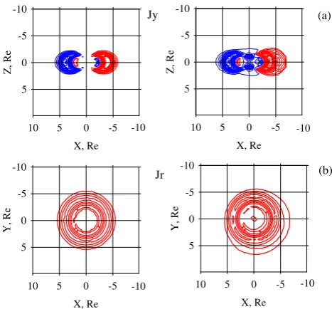
Figure 1 shows schematically the isolines of (a) jy in the noon-midnight meridional plane and (b)jR=

q

jx2+jy2 in the equatorial plane for a symmetric ring current (left panel), corresponding to quiet conditions and an asymmet-ric ring current (right panel) for disturbed conditions. The blue color indicates current flowing into and red color cur-rents out from the plane. Eastward and westward flow-ing components of the rflow-ing current are present both for quiet and disturbed conditions. Asymmetry is pronounced on the nightside. The parameters used to create this plot were R0east=2RE, R0west=4RE, σR=0.8, A=1, and J0east=1.5 nA/m2,J0west=3 nA/m2 for the symmetric case andR0part=6RE,J0part=2 nA/m2andδ =0◦for the asym-metric case.

2.2 Addition of a new tail current sheet

For the tail current system we introduce both global and lo-cal changes. Global changes include intensification of the tail current sheet as a whole using a tail current amplifica-tion factor(1+AT S)(Ganushkina et al., 2002b). This fac-tor indicates the change in the tail current from the original value, i.e. that given by Tsyganenko T89Kp=4, to values both lower (AT S<0) and higher (AT S>0) than the standard model. A new, thin tail current sheet is added to account for the local changes. The azimuthal componentAT of the vec-tor potential giving the tail current sheet in the Tsyganenko

-5 0 5 10

X, Re -10

-5

0

5

Y,

Re

-5 0 5 10

X, Re -10

-5

0

5

Y, R

e

Jr

-5 0 5 10

X, Re -10

-5

0

5

Z, Re

-5 0 5 10

X, Re -10

-5

0

5

Z, Re

Jy (a)

(b)

-10 -10

-10 -10

Fig. 1. The isolines of (a)jyin the noon-midnight meridional plane

andjR= q

jx2+jy2in the equatorial plane for symmetric ring current (left panel) corresponding to quiet conditions and asymmetric ring current (right panel) for disturbed conditions. Blue color indicates current flowing into and red color currents out from the plane.

T89 model has the form:

AT = W (x, y)

ST(z, aT, D0)+aT +ξT(z, D0) ×

C1+

C2

ST(z, aT, D0)

, (5)

whereC1andC2are the coefficients which define the current distribution in the central current sheet,aT is the radial scale length which defines the geocentric distance to the current density maximum, andD0 is the half-thickness of the cur-rent sheet in the central magnetotail region (for details, see Tsyganenko (1989)). The truncation factorW (x, y)is given in SM coordinates by

W (x, y)=0.5 1− x−x0

(x−x0)2+Dx2 1/2

! ×

1+y2/Dy2 −1

, (6)

wherex0is the coordinate which defines the location of the region of steepest decrease ofW (x, y),Dx andDy are the scale lengths corresponding to variations ofW (x, y)along

X- andY-directions.

We introduce two vector potentials,

AT1=

W1(x, y)

ST +aT +ξT

C1+

C2

ST

and

AT2=

W2(x, y)

ST +aT +ξT

C1+

C2

ST

20

10

0

-10

-20

-30

-40

Xgsm, Re

-150

-100

-50

0

50

100

150

200

250

In

te

g

ra

l c

u

rr

en

t,

mA

/m

T89

thin CS T89 + thin CS

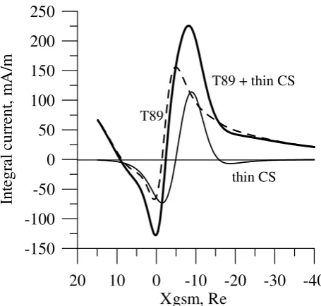
Fig. 2.xGSM-dependence of the integral current for the T89 model Kp=4 (dotted line), for the additional, relatively thin current sheet (thin solid line), and the combined T89 model with the added thin current sheet (thick solid line).

where the truncation factors are

W1(x, y)=

Ant c 1−

x−x1nt c

(x−x1nt c)2+Dx2 1/2

!

×1+y2/Dy2 −1

and

W2(x, y)=

Ant c 1−

x−x2nt c

(x−x2nt c)2+Dx2 1/2

!

×1+y2/Dy2 −1

(8)

The differenceAT1−AT2gives a vector potential character-ized by a finitex-scale; it is zero outside 25RE. Further-more, this vector potential produces a relatively thin current sheet. The current sheet is defined by four parameters: the amplitudeAnt c, which defines the thin current sheet intensity, x1nt candx2nt cdetermine the spatial distribution of functions W1andW2and give the points of steepest increase of these functions, and the half-thickness of the current sheet (D0). Other parameters are as in the T89 tail current module.

Figure 2 shows thexGSM-dependence of the Z-integrated current for the T89 modelKp=4 (dotted line), and for the additional thin current sheet (thin solid line). The thick solid line shows the combined T89 model and the additional thin current sheet. When the thin current sheet is added to T89 model, the integrated current maximum value is increased and its position is shifted tailward. The combination of the global variation of the tail current and the added new thin current sheet makes it possible to account for the magnetic field changes associated with substorms during the storm.

Table 1. Model parameters.

Ring current Tail current Magnetopause currents

R0east AT S RT

R0west Antc AMP

R0part x1ntc J0east x2ntc

J0west D0

J0part

σR

A δ

2.3 Magnetopause currents

The magnetopause moves inward during increased solar wind dynamic pressure. To adjust for this, the mag-netic field of the Chapman-Ferraro currents BCFT89 at the

magnetopause given by T89 Kp=4 model was scaled by BCF=χ3BCFT89, whereχ=(Pd/<Pd>)

k_,k=1/6,P dis the solar wind dynamic pressure, and <Pd>=2 nPa (Tsyga-nenko, 2002b). Self-similar compression/expansion of the magnetopause in response to changes inPd and scaling of its linear dimensions by the factor χ allow us to make a similar scaling for field components. The scaling parameter

AMP=χ3 is directly determined from solar wind pressure variations.

In the T89 model, the parameterRT defines the character-istic scale size of the magnetotail. In the T89Kp=4 model its value isRT=30RE. Using this model with zero tilt an-gle we determined the “magnetopause” position ZT ,T89 at

XGSM=−20REandYGSM=0. We then determined the mag-netopause position as given by Shue et al. (1998) model

ZT ,Shue, using the observed solar wind and IMF parameters. The magnetotail size is then modified by changing the value ofRT to 30RE·ZT ,Shue/ZT ,T89. As the magnetopause po-sition in the Shue et al. (1998) model depends on the solar wind dynamic pressure and IMFBz, theRT parameter is thus defined by the observed solar wind and IMF parameters.

Table 1 lists the model parameters for the three current sys-tems: the ring current, the tail current, and the magnetopause currents.

2.4 Modelling procedure

For modelling the storm events we use the Tsyganenko T89

accordance to Lui et al. (1987) study where AMPTE/CCE data were used to obtain perpendicular current character-istics during storms. The width of the Gaussian distribu-tion σR=0.8 and the anisotropy index A/2=1 are used for all three components of the ring current representation. The

σR=0.8 gives the rate of increase (decrease) in current den-sity distribution so that all the notable current would be in-cluded in between 2 and 6RE. A/2=1 was set following the Garcia and Spjeldvik (1985) study on anisotropy of par-ticle distribution, and it means that current density is concen-trated near the equator and decreases away from the equator. For the additional thin current sheet we setx1nt c=−2.0RE, x2nt c=−10.0 RE, andD0=0.2RE. With these values of pa-rameters for the additional thin current sheet the total tail cur-rent starts to deviate from the T89 value at about−5RE, and returns back to T89 value after−15RE(see Fig. 2).

Three parameters are computed from the observed so-lar wind data and Dst index. In the partial ring cur-rent representation, the parameterδ defining the duskward rotation depends on the corrected ring current index

D∗_st:δ=π 2t anh

|Dst∗|

Dst∗

0

, where Dst∗₀=41.6 nT (Tsyganenko, 2002b). The scaling parameterAMP for the magnetic field of the magnetopause currents and the scale size of the magne-totailRT were obtained from the solar wind data as described above.

The free parameters in the model, which are marked by bold font in Table 2, are the radius of the westward ring current (R0west) and partial ring current (R0part) and the maximum current densities for westward (J0west) and par-tial (J0part) ring currents, the amplification factor for the tail current (ATS), and the amplitude of additional thin current sheet intensity (Antc). We then searched the values of the free parameters that give the best fit between the model and the in-situ magnetic field observations by GOES 8, GOES 9, Polar, Geotail and Interball satellites (obtained from the Coordinated Data Analysis Web (CDAWeb) and DARTS at the Institute of Space and Astronautical Science (ISAS) in Japan), and theDst measurements (obtained from the World Data Center C2 for Geomagnetism, Kyoto).

The details of the fitting procedure are the following (Ganushkina et al., 2002b): The search procedure is initiated from different sets of initial values of the model parameters randomly generated using the Monte-Carlo method. The set of parameters which gave the minimum error between the model and the observed magnetic field values was selected as the starting point. After that, one of the parameters was var-ied while others were held fixed, in order to find the parame-ter value that gave the minimum error between the model and the observations. Next, using the optimum value for that pa-rameter, the next parameter was varied. The procedure was repeated for all free parameters. As a result, we obtain a set of parameters corresponding to the minimum error between observations and model. The procedure was repeated once more, but the parameters were varied in the vicinity of the previously obtained values, with a smaller step size to bet-ter localize the minimum. The possibility of finding a local

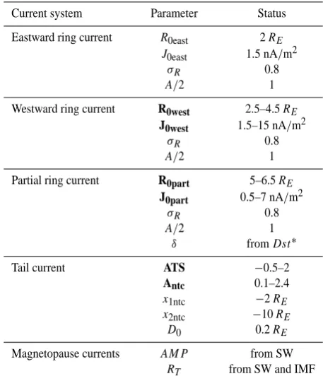
Table 2. Model parameters for storm event modelling.

Current system Parameter Status

Eastward ring current R0east 2RE J0east 1.5 nA/m2

σR 0.8

A/2 1

Westward ring current R0west 2.5–4.5RE J0west 1.5–15 nA/m2

σR 0.8

A/2 1

Partial ring current R0part 5–6.5RE J0part 0.5–7 nA/m2

σR 0.8

A/2 1

δ fromDst∗

Tail current ATS −0.5–2

Antc 0.1–2.4

x1ntc −2RE

x2ntc −10RE

D0 0.2RE

Magnetopause currents AMP from SW RT from SW and IMF

rather than a global minimum is reduced by combining two methods: first, the Monte-Carlo method that gives a random distribution of parameter values and then, the minimization procedure. Furthermore, the error value was controlled for each step of the calculations.

To obtain the model Dst index, the magnetic field from the extraterrestrial currents was computed at the locations of several stations such as Sun Juan, Tenerife, Tbilisi, Lunping, Kakioka, Honolulu and Del Rio. However, before the model values can be compared with the observed ones, the quiet time level must be subtracted from the model. This is done by modelling the entire duration of the quietest day of the month for each storm event. The quiet level of the magnetic field given by the model is then evaluated at the locations ofDst stations. In order to be able to examine the contributions of the different current systems to theDst index, the quiet-time levels are also evaluated for the ring, tail and magnetopause currents separately. Currents in the magnetosphere induce currents in the electrically conducting Earth, which are esti-mated to be about 25% of the measuredDst (H¨akkinen et al., 2002). In comparing our modelDst with the observed one, we remove this 25% from the observedDst.

3 Description of events

-20 -10 0 10 20

IM

F

B

z,

nT

0 8 16

Ps

w

, nPa

May 2, 1998

0 1000 2000

A

E

, nT

May 4, 1998

November 6-7, 1997 -80

-40 0 40

Ds

t,

n

T

-20 -10 0 10

IMF

B

z,

n

T

0 4 8 12

P

sw

, nP

a

October 10-12, 1997

0 400 800 1200 1600

AE,

n

T

-160

-120-80

-400

Ds

t,

n

T

-40 -20 0 20 40

IMF

B

z,

n

T

0 20 40

Ps

w

, nPa

0 1000 2000 3000

A

E

, nT

-300 -200 -100 0

Ds

t,

n

T

-20 -10 0 10 20

IM

F

B

z,

n

T

0 4 8 12

Ps

w

, nPa

0 400 800 1200

A

E

, nT

-160

-120-80

-400

40

Ds

t,

n

T

18 24 6 12 18 24 UT

0 12 24 12 24 UT

(a) (b)

(c) (d)

0 4 8 12 16 20 24 UT

0 4 8 12 16 20 24 UT

Fig. 3. Overviews (panels from top to bottom in each figure: IMFBzandPswas measured by WIND spacecraft,AEandDst) of four storm events that occurred on (a) 2 May 1998, (b) 4 May 1998, (c) 10–12 October 1997, and (d) 6–9 November 1997.

The storms in early May 1998 were initiated from an ex-tended period of solar activity which started on 29 April 1998. There were several coronal mass ejections during the period: on 29 April (17:00 UT), 1 May (23:40 UT), 2 May (05:30 UT) and 4 May (02:00 UT). The activity on 2 May 1998 (Fig. 3a) was driven by a magnetic cloud, whose ef-fects were first seen at about 03:35 UT, when IMFBzturned southward. There were several pressure pulses reaching up to about 15 nPa. The magnetospheric response was seen as a strong increase in theAEindex that reached over 20:00 nT at about 12:00 UT. TheDst index reached about−80 nT at 15:00 UT and recovered to the level of about−50 nT by the end of the day.

The storm on 10–12 October 1997 was moderate in inten-sity (Fig. 3c). The IMFBzremained negative (−12 nT) until about 10:00 UT on 11 October. A solar wind dynamic pres-sure peak of about 10 nPa was detected at about 22:00 UT on 10 October. TheAEindex showed several peaks with more than 1000 nT magnitude during the main phase and storm maximum. Dst reached−140 nT at about 03:00 UT on Oc-tober 11 and recovered to−20 nT by the end of the day.

A storm of about similar intensity occurred on 6–7 November 1997 (Fig. 3d). On 6 November Bz fluctuated around zero and dropped to −15 nT at the end of the day around 23:00 UT. Solar wind dynamic pressure was about 3 nPa during 6 November and increased up to about 10 nPa at about 22:00 UT. The AEindex had several peaks, with the highest magnitude of about 1000 nT at the beginning of 7 November. Dst reached−120 nT at about 04:00 UT on 7 November and recovered to−20 nT by the end of the day.

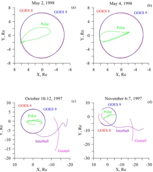
Figure 4 shows the evolution of orbits of satellites such as GOES 8 (red curve), GOES 9 (blue curve), Polar (green curve), Geotail (pink curve) and Interball (purple curve), dur-ing the time periods when the magnetic field data was used for modelling storm events on (a) 2 May 1998, (b) 4 May 1998, (c) 10–12 October 1997, and (d) 6–9 November 1997.

4 Model results

4.1 Magnetic field andDst index

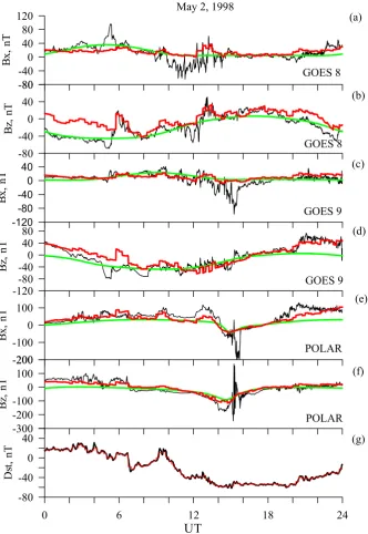
Figure 5 shows the model results for the storm on 2 May 1998. The Bx and Bz components (GSM coordinates) of the external magnetic field are shown in solid black lines for GOES 8 (a, b), GOES 9 (c, d), and Polar (e, f). The By is not shown since theBxandBzcomponents represent the most changes in the main current systems occurring during storm times, and our model does not include separate repre-sentation for field-aligned currents. Our storm time model is shown in red and the Tsyganenko T89 model forKp=4 in green. Bottom panel (g) shows the measuredDst index (black line) andDstas calculated using our storm time model (red line). Figure 6 shows the results for the 4 May 1998 storm in the same format as Fig. 5.

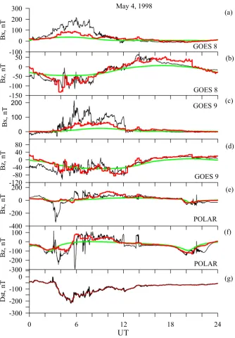
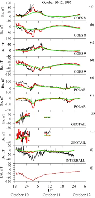
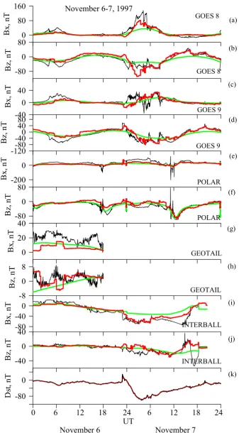
Figure 7 shows the measured and modeled magnetic field in the same format as Fig. 5, with the addition of theBxand Bz components of the external magnetic field from Geotail (g, h) andBxcomponent from Interball (i) for the 10–12 Oc-tober 1997 storm event. TheBz component from Interball was not available during this time. Figure 8 shows the model results for the 6–7 November 1997 storm in the same format as Fig. 7.

Our storm-time magnetic field model reproduces the ob-servedDst index almost perfectly for all modeled storms. The Bz component at geostationary orbit is also quite well reproduced, including the substorm-associated changes. Model curves forBzcomponent follow quite closely the ob-served ones also at Polar, Geotail and Interball. On the other hand, our model cannot fit well the observed large variations

in the Bx component. The large observed Bx values im-ply the existence of intense currents that can be either field-aligned or perpendicular, or an even stronger compression of the magnetosphere than that represented by the magne-topause current intensification in our model.

4.2 Model parameters

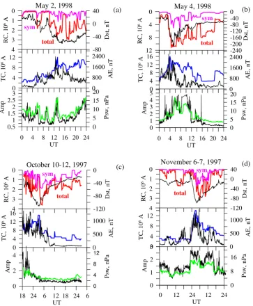
Figure 9 shows the time evolution of the model parameters. The four plots show the results for the four storm events (in each figure): symmetric ring current intensity (pink line) and total ring current intensity including symmetric and partial components (red line), together with variation of theDst in-dex (black line), tail current intensity (blue line), together with theAEindex (black line), and amplification factor for magnetopause currentAMP (green line) with the observed solar wind dynamic pressure (black line).

The ring current intensity tends to follow theDst index. Our model produces a very sharp and large increase in the ring current intensity during the storm main phase on 4 May 1998, when the relative role of the ring current inDst also strongly increases. The tail current responds with its in-tensity increase to substorm activity represented by theAE

index. The amplification factor for the magnetopause cur-rent magnetic field AMP was computed from solar wind dynamic pressure, which is reflected in the similar temporal evolution of the two curves.

Maximum tail current intensity value ranged from about 10·106A on 2 May 1998 to 20·106 A on 4 May 1998. On the other hand, maximum ring current intensity was around 3·106A during all three moderate storms, but during the in-tense storm on 4 May 1998, the ring current intensity was 11·106A, sometimes reaching values higher than the tail cur-rent.

The partial ring current plays a significant role. The total ring current intensity was 3·106A for moderate storm maxi-mum and 10·106A for intense storm maximum. At the same time, the symmetric ring current values were 1.8·106A and 3.9·106A, respectively.

4.3 Contributions toDst index

8 4 0 -4 -8 X, Re

-8 -4 0 4 8

Y

,

R

e

May 2, 1998

GOES 8 _{GOES 9}

Polar

8 4 0 -4 -8

X, Re -8

-4 0 4 8

Y

,

R

e

May 4, 1998

GOES 8 _{GOES 9}

Polar

10 0 -10 -20

X, Re -20

-15 -10 -5 0 5 10

Y

,

R

e

October 10-12, 1997

GOES 8

GOES 9

Polar

Geotail Interball

10 0 -10 -20 -30

X, Re -30

-20 -10 0 10

Y

,

R

e

November 6-7, 1997

GOES 8 GOES 9

Polar

Geotail Interball

(a) (b)

(c) (d)

Fig. 4. Evolution of orbits of satellites during the time periods when the magnetic field data was used for modelling storm events on (a) 2 May 1998, (b) 4 May 1998, (c) 10–12 October 1997, and (d) 6–9 November 1997.

obtained model values for the quiet time ring current were 0.2 to 3 nA/m2, which is in agreement with previous ob-servations (Lui and Hamilton, 1992) and modelling (Milillo et al., 2003).

Figure 11 shows contributions from the ring current (red line), tail current (blue line) and magnetopause currents (green line) to the observed Dst index (black line) during the four storm events. For the two consecutive storms on 2 May and 4 May 1998, it is clear that the contributions from different current systems to theDst index change during the storm development: the ring current contribution gradually increases and reaches maximum at the intense storm maxi-mum, whereas the tail current contribution does not show a clear increase with storm development on 4 May. During the moderate storm on 3 May, the tail current contributes more than the ring current to theDst. The situation is quite dif-ferent during the intense storm on 4 May: It is clearly seen that then the main contribution toDst comes from the ring current. For the 10–12 October 1997 storm, the main contri-bution to theDst comes from the tail current after the storm beginning until the maximum. At the beginning of the recov-ery phase the ring current becomes dominant and remains

dominant until the end of the storm. During the entire 6–7 November 1997 storm, the main contribution toDst index comes from the tail current. These results suggest that the relative contributions from different current systems to the

Dst index depend on the storm intensity such that the ring current dominates during strong storms while the tail current is important during moderate storms. Note that for all storms the tail current intensifies first at the storm beginning when theDstdrops, while the ring current develops later and stays longer at an increased level.

5 Discussion

-80 -40 0 40 80 120

Bx

,

n

T

GOES 8

-80 -40 0 40 80

Bz

,

n

T

-120-80

-400

40

Bx

,

n

T

-120 -80 -40 0 40 80

Bz,

n

T

GOES 9 May 2, 1998

-200 -100 0 100

Bx

,

n

T

-300 -200 -100 0 100 200

Bz

,

n

T

GOES 8

GOES 9

POLAR

POLAR

0 6 12 18 24

UT

-80 -40 0 40

Ds

t,

n

T

(a)

(b)

(c)

(d)

(e)

(f)

(g)

Fig. 5. Modelling results for 2 May 1998 (panels from top to bottom):BxandBzcomponents of the external magnetic field measured (solid black lines) on GOES 8 (a, b) and GOES 9 (c, d), on Polar (e, f), calculated using our storm time model (red lines) and T89Kp=4 (green lines), and measured (black line) and calculated (red line)Dst-index (g).

magnetopause, and varied the dayside magnetopause cur-rents. The key new features in this paper are the introduction of an eastward ring current and a partial ring current with closure by Region 2 field-aligned currents, in addition to the westward symmetric ring current. Furthermore, a new time-variable thin cross-tail current has been added to the model. This combination allows us to simultaneously describe the substorm-associated tail field variations and the storm-driven ring current intensity changes. Magnetic field observations by GOES 8, GOES 9, Polar, Geotail and Interball, and the

Dst measurements were used to evaluate the model parame-ters for each time step individually.

-100 0 100 200 300

Bx

,

n

T

GOES 8

-150 -100 -50 0 50

Bz

,

n

T

0 100 200

Bx

,

n

T

-120 -80 -40 0 40 80

Bz,

n

T

GOES 9 May 4, 1998

-400 -200 0 200

Bx

,

n

T

-300 -200 -100 0 100

Bz

,

n

T

GOES 8

GOES 9

POLAR

POLAR

0 6 12 18 24

UT

-200 -100 0

Ds

t,

n

T

(a)

(b)

(c)

(d)

(e)

(f)

(g)

Fig. 6. Same as in Fig. 5 but for 4 May 1998 storm event.

unlikely that large Bx values are due to localized current systems, such as field-aligned currents, asBx remains large quite a long time and field-aligned currents typically occupy more narrow region in local time. There is a correspondence between the times when largeBx is observed on the night-side and the times when there are peaks in solar wind dy-namic pressure (see Fig. 3 and Figs. 5–8). These largeBx values are most probably created by strong compression of the magnetosphere, which is only partially represented in the model by the intensification of the magnetopause currents.

The model ring current intensity follows closely theDst index, which is partly but not totally a consequence of us-ingDst as input data in the model. Our tail current inten-sifies as substorm activity represented by theAE index

-40

0

40

80

120

B

x

, n

T

GOES 8

-160

-80

0

80

Bz

,

n

T

-40 0 40

Bx

,

n

T

-120

-80

-40

0

40

80

Bz,

n

T

GOES 9

October 10-12, 1997

0

100

B

x

, n

T

-200

-100

0

100

Bz

,

n

T

GOES 8

GOES 9

POLAR

POLAR

-120

-80

-40

0

40

Dst

,

n

T

-80

-40

0

40

80

B

x

, n

T

-20

0

20

Bz,

n

T

-60

-40

-20

0

20

Bx

,

n

T

18 24 6 12 18 24 6

UT

October 10 October 11 October 12

GEOTAIL

INTERBALL

GEOTAIL

(a)

(b)

(c)

(d)

(e)

(f)

(g)

(h)

(i)

(j)

0

80

160

B

x

, n

T

-80

0

80

B

z, n

T

-40

0

40

Bx,

nT

-120

-80

-40

0

40

80

Bz,

n

T

GOES 9

November 6-7, 1997

-200

0

B

x

, n

T

-80

0

80

Bz

,

n

T

GOES 8

GOES 9

POLAR

POLAR

-80

0

Ds

t, n

T

0

20

40

B

x

, n

T

-8

0

8

Bz

,

n

T

-80

-40

0

Bx,

nT

0 6 12 18 24 6 12 18 24

UT

November 6

November 7

INTERBALL GEOTAIL

-40

0

40

Bz,

n

T

INTERBALL (a)

(b)

(c)

(d)

(e)

(f)

(g)

(h)

(i)

(j)

(k)

4 3 2 1 0 RC, 10

6 A

-80 -40 0 40 Ds t, nT 0 4 8 12 TC , 10

6 A

0 800 1600 2400 AE , n T

May 2, 1998

0.5 1 1.5 2 2.5 3 Am p 0 5 10 15 20 Ps w , n Pa

0 4 8 12 16 20 24 UT 12 8 4 0 RC, 10

6 A

-240 -200 -160 -120 -80 -40 0 Ds t, n T 0 4 8 12 16 TC , 10

6 A

0 800 1600 2400 AE , n T

May 4, 1998

0 1 2 3 4 5 Am p 0 5 10 15 20 Ps w , n Pa

0 4 8 12 16 20 24 UT 4 3 2 1 0 RC, 10

6 A

-120 -80 -40 0 Ds t, n T 0 4 8 12 16 TC , 1 0

6 A

0 500 1000 AE , n T

October 10-12, 1997

0 2 4 Am p 0 4 8 12 Ps w , n Pa

18 24 6 12 18 24 6 UT 4 3 2 1 0 RC, 10

6 A

-120 -80 -40 0 40 Ds t, n T 0 4 8 12 TC , 10

6 A

0 500 1000

AE

, nT

November 6-7, 1997

0 1 2 3 Amp 0 8 16 Ps w , n Pa

0 12 24 12 24 UT (a) (b) (c) (d) total sym total sym sym total total sym

Fig. 9. Time evolution of the model parameters (in each figure): (upper panel) symmetric ring current (pink line) and asymmetric ring current including symmetric and partial components intensity (red line), together with variation ofDstindex (black line), (middle panel) tail current intensity (blue line), together withAEindex (black line), and (bottom panel) amplification factor for magnetopause current magnetic field AMP(green line) with the observed solar wind dynamic pressure (black line) for (a) 2 May 1998, (b) 4 May 1998, (c) 10–12 October 1997, and (d) 6–9 November 1997 storm events.

The tail currents intensify because of the strong driving (compare Fig. 11 to IMFBz in Fig. 3). As theAE index includes both the driven system, as well as the substorm-associated currents, it intensifies strongly as the driving in-creases. As we are looking at the storm evolution in a rather coarse time resolution, theAEindex is the appropriate com-parison, and the correlation is positive: the tail currents inten-sify for increasingAE. On the other hand, a more fine time resolution comparison of the substorm-associated cross-tail current variations should show an anti-correlation with the substorm-associatedAEindex.

-30 -20 -10 0 10 20

Dst

, nT

November 29, 1997, quiet day

mp

rc

tc

0 2 4 6 8 10 12 14 16 18 20 22 24 UT

-8 -4 0 4

Ds

t,

nT

Fig. 10. Contributions from the ring current (red line), the tail cur-rent (blue line) and the magnetopause curcur-rents (green line) to the ob-servedDstindex (black line) and (lower panel) the observed (black line) and model (purple line)Dst index during 29 November, the quietest day of November 1997.

The eastward ring current at the inner edge provides an improved response of the current changes in theDst index, while its effects are quite small in the magnetic field mea-surements of the high-altitude spacecraft. Thus, as theDst index is a measure of the integrated total intensity of the cur-rents in the magnetosphere, the eastward ring current pro-vides a substantial improvement. The partial ring current in our model is located near the outer edge of the symmetric ring current in the evening sector, and its intensity is thus largely defined by the geostationary orbit magnetic field mea-surements that record the strongest variations of currents in that region. Our total ring current representation is in agree-ment with the recent study by Le et al. (2003) on the mor-phology of the ring current derived from magnetic field ob-servations. Figure 12 illustrates the changes in the model current density in nA/m2in the (a) equatorial and (b) noon-midnight meridian planes for three moments during the 4 May 1998 intense storm: (left) before the storm at 01:00 UT, (middle) at the storm main phase at 05:00 UT and (right) during the recovery phase at 10:00 UT. It can be seen how the ring and tail currents intensify and how the ring current becomes asymmetric with maximum near dusk at the storm main phase and recovers its symmetry during the recovery phase. Our model gave the total ring current intensity as 3·106A for moderate storm maximum and 10·106A for in-tense storm maximum, and the symmetric ring current val-ues were 1.8·106A and 3.9·106A, respectively. This means that a large part (40% and 60%, respectively) of the intensity of the total ring current comes from the partial ring current. On the other hand, as we do not have good local time cov-erage of the inner magnetosphere magnetic field measure-ments, the distinction between symmetric and asymmetric parts is sometimes difficult. However, without better

cover-age of observations, there is little that can be done to address this ambiguity.

During moderate-intensity storms, the tail current con-tributed to theDst index more than the ring current. This re-sult is consistent with the study by Dremukhina et al. (1999), who studied four moderate storms. On the other hand, Turner et al. (2000), using the Tsyganenko T96 magnetospheric magnetic field model to model one moderate January 1997 storm, concluded that the tail current contribution is about 25% of the measuredDst variation. For 2 May 1998, and 6–7 November 1997, the tail current contribution almost fol-lows the observed Dst index, whereas on 10–12 October, 1997, the ring current is dominant during the storm recov-ery phase. On 4 May 1998, during the vrecov-ery intense storm, the ring current was dominant and also gave the largest con-tribution to theDst index. Comparing the two consequent storms on 2 May and 4 May 1998, the tail current intensifi-cation was quite comparable during both storms, while ing 4 May the ring current was much more intense than dur-ing the 2 May storm. Furthermore, durdur-ing the 4 May storm, the magnetosphere was in a highly compressed state (Russell et al., 2000), which also contributed to the inner magneto-sphere field variations. Thus, during intense storms the main contribution to the Dst index comes from the ring current, but during moderate storms the tail current contribution can be dominant or comparable to the ring current. Our results are similar to earlier work (Alexeev et al., 1996; Dremukhina et al., 1999) with regard to moderate storms, but give a quite different picture of the dynamics during intense storms.

When discussing the relative contributions from the ring and tail currents, the key question is how to separate partial ring current and tail current at the inner edge of the plasma sheet. Alexeev et al. (1996), Dremukhina et al. (1999), and Arykov and Maltsev (1994) assumed that the current flowing in the region at 6–8REis a tail current. At the same time, Le et al. (2003) state that current in this region is a partial ring current.

0 6 12 18 24 UT

-80 -40 0 40 80

Ds

t,

n

T

May 2, 1998

mp

rc

tc

0 6 12 18 24

UT -300

-200 -100 0 100

Ds

t,

n

T

May 4, 1998

-120 -80 -40 0 40

Ds

t,

n

T

mp

mp

mp

-120 -80 -40 0 40

Ds

t,

n

T

18 24 6 12 18 24 6 UT

0 6 12 18 24 6 12 18 24 UT

October 10-12, 1997 November 6-7, 1997

rc

rc

rc

tc

tc tc

(a) _(b)

(c) (d)

Fig. 11. Contributions from the ring current (red line), the tail current (blue line) and the magnetopause currents (green line) to the observed Dst-index (black line) during (a) 2 May 1998, (b) 4 May 1998, (c) 10–12 October 1997, and (d) 6–7 November 1997 storm events.

by Le et al. (2003), and the tail current was not subtracted from the measurements. Therefore, it is important to real-ize that results indicating strong asymmetric ring current and strong inner-tail current are not contradictory but may be the same physical process described with different terminology.

It is interesting to note that our model current systems have different characteristic response times. While the ring cur-rent increases quite slowly (much slower than theDst en-hancement), the tail current responds very rapidly. Thus, most of the fast decrease in theDst index during the storm main phase in this model is created by the intensifying cross-tail current. The ring current intensification contributes to the magnitude and timing of the storm maximum, as the ring current maximizes at storm maximum. Further analysis on the relative contributions toDst from the different current systems including the ring and tail current contributions dur-ing storm recovery phase and the contribution of the magne-topause currents is still needed. In particular, one of the still open issues is how the different solar wind drivers affect the evolution of the magnetospheric current systems: for exam-ple, are the current systems during magnetic clouds similar to those produced by highly fluctuating solar wind and IMF conditions (Huttunen et al., 2002)?

The model presented here is an empirical model, where the temporal evolution is determined from the observed mag-netic variations. The modelling method is an extension of the work by Pulkkinen et al. (1992), providing an improved time-varying representation of the inner magnetosphere field.

Furthermore, while Pulkkinen et al. (1992) modeled individ-ual substorm phases lasting typically 1–2 h using a single set of parameter values that changed in a linear manner, here the modelling covers several storms each lasting of the order of 24 h, and the model parameters are defined for each time step individually, with no forced relationship of the parame-ter values between subsequent time steps.

Fig. 12. The model current density in nA/m2in the (a) equatorial and (b) noon-midnight meridian planes for three moments during 4 May 1998 intense storm: (left) before the storm at 01:00 UT, (middle) at the storm main phase at 05:00 UT and (right) during the recovery phase at 10:00 UT.

An important feature of paraboloid model (Alexeev et al., 2001) is that it describes the magnetic field of each current system as a function of its own time-dependent parameters which are determined from satellite and ground-based data. Because both Alexeev’s model and our models contain time-dependent parameters, it would be very useful and interesting to compare the modelling results. It is planed to do the mod-elling of several storm events using both models in the near future. This will be a topic for another paper.

A third approach to defining the storm-time inner magne-tosphere current distribution was adopted in the T02 model

model details faster field variations associated with substorm activity in the tail than the T02 model. Furthermore, it ap-pears that the T02 model reproduces quite well the observed magnetic field during moderate storms, but during the very intense storm on 4 May 1998, the T02 model produced a very strong Bz at GOES 8 and 9 of −300 nT, instead of the observed−100 nT. This is most probably caused by the very small number of such intense storms in the statistical database used to derive the model parameters. Thus, at times of highly atypical behavior, the event-oriented models, which adjust the parameters according to in-situ observations, can provide higher accuracy.

The time variations of the current systems during storms allows us to discuss one of the key open issues in storm re-search, namely the role of substorms in the storm evolution (see, e.g. McPherron, 1997). We have shown that theAE -enhancements are associated with strong intensification of the tail current, in a manner analogous to the isolated sub-storms (see, e.g. Baker et al., 1996). This would imply that most substorms during storms have similar tail current sys-tem development as during isolated substorms. This is con-sistent with the study of Pulkkinen et al. (1992), where a sub-storm during a moderate sub-storm was found to have a current sheet that was located closer to the Earth and more intense than during isolated substorms, but the temporal evolution was quite similar. On the other hand, Pulkkinen et al. (2002) found that only a portion of the storm-time substorms be-have similarly to the isolated ones. The auroral electrojet expanded sometimes poleward but in many cases also equa-torward. The storm-time energetic particle fluxes show large fluctuations, quite different from isolated substorm injections (Reeves and Henderson, 2001). Using the time-evolving model developed here with a higher time resolution during storm-time substorms will allow us in the future to examine the storm-substorm relationship in more detail.

6 Conclusions

We presented an empirical, temporally evolving magnetic field model for storm periods. The model describes the ring current, the tail current, and the magnetopause currents with functions containing free parameters, whose values are de-fined for each time step separately based on in-situ measure-ments in the magnetosphere, on solar wind dynamic pres-sure, and on the ground-based storm indexDst. We modeled the magnetic field evolution during four storms: 2 May and 4 May 1998, 10–12 October 1997, and 6–7 November 1997. The storm-time magnetic field model reproduced quite well large-scale variations of currents and magnetic field, while the smaller scale variations would require the introduction of localized currents not included in this model. Of the model parameters, the ring current intensity followed theDst index and the tail current intensity followed theAEindex, which lends support to the conclusion that our model indeed re-produces the field variations associated with storms and sub-storms.

The model results show quite consistent behavior during the four modeled storms. The tail current intensifies first, and follows the drop in theDst index. The ring current de-velops slower, and stays at an increased level longer than the tail current. During moderate storms (Dst>−100–150 nT), both ring and tail currents are intensified, but the tail cur-rent contributes more toDst than the ring current. On the other hand, during intense storms (Dst>−200 nT), the tail current is intensified, but remains nearly constant, while the ring current follows theDstvariations. During these periods, the main contribution to theDst index comes from the ring current. Thus, the information contained in theDst index is different during small and large storms.

Acknowledgement. We would like to thank K. Ogilvie and R. Lep-ping for the use of WIND data in this paper, Interball-tail MIF-M team for providing high resolution data (routinely produced by S. Romanov), World Data Center C2 for Geomagnetism, Kyoto, for the provisionalAE,KpandDst indices data. The data were obtained from the Coordinated Data Analysis Web (CDAWeb). GEOTAIL magnetic field data were provided by T. Nagai through DARTS at the Institute of Space and Astronautical Science (ISAS) in Japan. This work was supported by the Academy of Finland.

References

Alekseyev, I. I.: Regular magnetic field in the Earth’s magneto-sphere, Geomagnetism and Aeronomy, 18, 447–452, 1978. Alexeev, I. I., Belenkaya, E. S., Kalegaev, V. V., Feldstein, Y. I., and

Grafe: A. Magnetic storms and magnetotail currents, J. Geophys. Res., 101, 7737–7747, 1996.

Alexeev, I. I., Kalegaev, V. V., Belenkaya, Bobrovnikov, S. Y., Feld-stein, Y. I., and Gromova, L. I.: Dynamic model of the magne-tosphere: Case study for January 9–12, 1997, J. Geophys. Res., 106, 25 683–25 693, 2001.

Arykov, A. A. and Maltsev, Yu. P.: Contribution of various sources to the geomagnetic storm field, Geomagnetism and Aeronomy, 33, 771–775, 1994.

Baker, D. N., Pulkkinen, T. I.: Angelopoulos, V., Baumjohann, W., and McPherron, R. L. The neutral line model of substorms: Past results and present view, J. Geophys. Res., 101, 12 975–13 010, 1996.

Chen, M. W., Schulz, M., Lyons, L. R., and Gorney, D. J.: Storm-time transport of ring current and radiation belt ions, J. Geophys. Res., 98, 3835–3849, 1993.

Dessler, A. J. and Parker, E. N.: Hydromagnetic theory of magnetic storms, J. Geophys. Res., 64, 2239–2259, 1959.

Dremukhina, L. A., Feldstein, Y. I., Alexeev, I. I., Kalegaev, V. V., and Greenspan, M. E.: Structure of the magnetospheric magnetic field during magnetic storms, J. Geophys. Res., 104, 28 351– 28 360, 1999.

Ebihara, Yu. and Ejiri, M.: Simulation study on fundamental prop-erties of the storm-time ring current, J. Geophys. Res., 105, 15 843–15 859, 2000.

Fok, M.-C. and Moore, T. E.: Ring current modeling in a realistic magnetic field configuration, Geophys. Res. Letters, 24, 1775– 1778, 1997.

Ganushkina, N. Yu., Pulkkinen, T. I., Kubyshkina, M. V., Singer, H. J., and Russell, C. T.: Modeling the ring current magnetic field during storms, J. Geophys. Res., 10.1029/2001JA900101, 02 July 2002b.

Ganushkina, N. Yu., Pulkkinen, T. I., Kubyshkina, M. V., and Singer, H. J.: Comparative study of magnetospheric configura-tion changes during May 2, 1998 moderate storm and May 4, 1998 intense storm events, in Proceedings of Sixth International Conference on Substorms, edited by Winglee, R. M., University of Washington, Seattle, 483–488, 2002c.

Ganushkina, N. Yu., and Pulkkinen, T. I.: Particle tracing in the inner Earth’s magnetosphere and the formation of the ring cur-rent during storm times, Advances in Space Research, 30, 1817– 1820, 2002.

Garcia, H. A., and Spjeldvik, W. N.: Anisotropy characteristics of geomagnetically trapped ions, J. Geophys. Res., 90, 347–358, 1985.

Huttunen, K. E. J., Koskinen, H. E. J., and Schwenn, R.: Variability of magnetospheric storms driven by different solar wind pertur-bations, J. Geophys. Res., 107, 10.1029/2001JA900171, 02 July 2002.

H¨akkinen, L. V. T., Pulkkinen, T. I., Nevanlinna, H., Pirjola, R. J., and Tanskanen, E. I.: Effects of induced currents on Dst and on magnetic variations at midlatitude stations, J. Geophys. Res., 107, SMP1-7, CitedID 1014, DOI 10.1029/2001JA900130, 2002.

Jordanova, V. K., Kozyra, J. U., Nagy, A. F., and Khazanov, G. V.: Kinetic model of the ring current-atmosphere interactions, J. Geophys. Res., 102, 14 279–14 291, 1997.

Le, G., Russell, C. T., and Takahashi, K.: Morphology of the ring current derived from magnetic field observations, accepted for publications to Annales Geophysicae, 2003.

Liemohn, M. W., J. U. Kozyra, M. F. Thomsen, A. J. Ridley, G. Lui, J. E. Borovsky, and Cayton, T. E.: Dominant role of the asym-metric ring current in producing the stormtime Dst*, J. Geophys. Res., 106, 10 883–10 904, 2001.

Lui, A. T. Y., McEntire, R. W.; Krimigis, S. M.: Evolution of the ring current during two geomagnetic storms, J. Geophys. Res., 92, 7459–7470, 1987.

Lui, A. T. Y. and Hamilton, D.C.: Radial profiles of quiet time mag-netospheric parameters, J. Geophys. Res., 97, 19 325–19 332, 1992.

McPherron, R. L.: The role of substorms in the generation of mag-netic storms, in: Geomagmag-netic Storms, Geophysical Monograph 98, edited by Tsurutani, B. T., Gonzalez, W. D., Kamide, Y., and Arballo, J. K., 131–147, 1997.

Milillo, A., Orsini, S., Delcourt, D. C., Mura, A., Massetti, S., De Angelis, E., and Ebihara, Y.: Empirical model of proton fluxes in the equatorial inner magnetosphere: 2. Properties and applica-tions, J. Geophys. Res., 108, 2002JA009581, 2003.

Pulkkinen, T. I., Baker, D. N., Pellinen, R. J., Buchner, J., Koski-nen, H. E. J., Lopez, R. E., Dyson, R. L., and Frank, L. A.: Par-ticle scattering and current sheet stability in the geomagnetic tail during the substorm growth phase, J. Geophys. Res., 97, 19 283– 19 297, 1992.

Pulkkinen, T. I., Koskinen, H. E. J., Huttunen, K. E. J., Kauristie, K., Tanskanen, E. I., Palmroth, M., and Reeves, G. D.: Effects of magnetic storms on substorm evolution, Sixth International Conference on Substorms, edited by R. M. Winglee, University of Washington, Seattle, 2002, 464–471.

Reeves, G. D., and Henderson, M. G.: The storm-substorm rela-tionship: Ion injections in geosynchronous measurements and composite energetic neutral atom images, J. Geophys. Res., 106, 5833–5844, 2001.

Roederer, J. G.: Dynamics of geomagnetically trapped radiation, 36 pp., Springer-Verlag, New York, 1970.

Russell, C. T., Le, G., Chi, P., et al.: The extreme compression of the magnetosphere on May 4, 1998, as observed by the Polar spacecraft, Adv. Space Res., 25, 1369–1375, 2000.

Sckopke, N.: A general relation between the energy of trapped par-ticles and the disturbance field near the Earth, J. Geophys. Res., 71, 3125–3130, 1966.

Shue, J.-H., Song, P., Russell, C. T., et al.: Magnetopause loca-tion under extreme solar wind condiloca-tions, J. Geophys. Res., 103, 17 691–17 700, 1998.

Tsyganenko, N. A.: Global quantitative models of the geomagnetic field in the cislunar magnetosphere for different disturbance lev-els, Planet. Space Sci., 35, 1347–1358, 1987.

Tsyganenko, N. A.: A magnetospheric magnetic field model with a warped tail current sheet, Planet. Space Sci., 37, 5–20, 1989. Tsyganenko, N. A.: Modeling the Earth’s magnetospheric magnetic

field confined within a realistic magnetopause, J. Geophys. Res., 100, 5599–5612, 1995.

Tsyganenko, N. A.: A model of the near magnetosphere with a dawn-dusk asymmetry: 1. Mathematical structure, J. Geophys. Res., 107, SMP 12-1, CiteID 1179, DOI 10.1029/2001JA0002192001, 2002a.

Tsyganenko, N. A.: A model of the near magnetosphere with a dawn-dusk asymmetry: 2. Parameterization and fitting to obser-vations, J. Geophys. Res., 107, SMP 10-1, CiteID 1176, DOI 10.1029/2001JA000220, 2002b.