Trunk detection based on laser radar and vision data fusion
Jinlin Xue
*,
Bowen Fan
,
Jia Yan
,
Shuxian Dong
,
Qishuo Ding
(College of Engineering, Nanjing Agricultural University, Nanjing210095, China)Abstract: Tree trunks detection and their location information are needed to perform effective production and management in forestry and fruit farming. A novel algorithm based on data fusion with a vision camera and a 2D laser scanner was developed to detect tree trunks accurately. The transformation was built from a laser coordinate system to an image coordinate system, and the model of a rectangle calibration plate with twoinward concave regions was established to implement data alignment between two sensors data. Then, data fusion and decision with Dempster-Shafer theory were achieved through integration of decision level after designing and determining basic probability assignments of regions of interesting (RoIs) for laser and vision data respectively. Tree trunk width was calculated by using laser data to determine basic probability assignments of RoIs of laser data. And a stripping segmentation algorithm was presented to determine basic probability assignments of RoIs of vision data, by calculating the matching level of RoIs like tree trunks. A robot platform was used to acquire data from sensors and to perform the developed tree trunk detection algorithm. Combined calibration tests were conducted to calculate a conversion matrix transforming from the laser coordinate system to the image coordinate system, and then field experiments were carried out in a real pear orchard under sunny and cloudy conditions, with trunk width measurement of 120 trees and 40 images processed by the presented stripping segmentation algorithm. Results showed the algorithm was successful to detect tree trunks and data fusion improved the ability for tree trunk detection. This algorithm could provide a new method for tree trunk detection and accurate production and management in orchards.
Keywords: trunk detection, data fusion, evidence theory, calibration, laser radar, vision camera DOI: 10.25165/j.ijabe.20181106.3725
Citation: Xue J L, Fan B W, Yan J, Dong S X, Ding Q S. Trunk detection based on laser radar and vision data fusion. Int J Agric & Biol Eng, 2018; 11(6): 20–26.
1 Introduction
Tree trunk detection and their location information are needed to perform effective production and management in forestry and fruit farming, such as fertilization, irrigation, weeding, spraying, pruning and harvesting operations[1,2]. At present, laser radar and
machine vision have been used as main device for detecting tree trunks[3-6]. Liang et al.[7] distinguished different data classes using
laser point cloud data, and then identify the class of data points of tree trunk through the detection of linear points in the vertical direction. Lehtomäki et al.[8] classified the LiDAR points on the
basis of cylinder feature to detect tree trunk and pole-like objects. Rahman and Gorte[9] proposed tree filtering approach to separate
dominant tree and undergrowth vegetation on the fact that a dominant tree has distinct parts in the histogram. Bargoti et al.[10]
presented a trunk localization pipeline for identification of individual trees in an apple orchard using a Hough Transform and a Hidden Semi-Markov Model. Hamner et al.[11] tendered a 2D
laser scanner based method to identify rows of trees by detect trunks and/or tree crown, and a Hough Transform was used to
Received date: 2017-08-17 Accepted date: 2018-02-06
Biographies: Bowen Fan, Master candidate, research interest: intelligent agricultural vehicle, Email: [email protected]; Jia Yan, Master candidate, research interest: intelligent agricultural vehicle, Email: [email protected];
Shuxian Dong, Master candidate, research interest: intelligent agricultural vehicle, Email: [email protected]; Qishuo Ding, PhD, Professor, research
interest: agricultural mechanization, Email: [email protected].
*Corresponding author: Jinlin Xue, PhD, Professor, Vice dean, research
interest: intelligent agricultural vehicle, College of Engineering, Nanjing Agricultural University, Nanjing 210095, China. Tel: 86-13813902501, Email: [email protected].
extract feature points and rows of tree for navigation of an agricultural vehicle. Guivant et al.[12] detected tree trunks by
using a two-dimensional laser scanner, and the detected tree trunk was regarded as landmarks to perform simultaneous localization and mapping algorithm. Also, 3D laser scanners have been applied to detect trees. Zhang et al.[13] proposed a method to
extract information of tree rows and trunks from 3D LiDAR point cloud data for an autonomous vehicle in orchards. However, 3D laser scanners have more expensive and more intensive computation than 2D laser scanners.
Also, vision sensors can be used to extract features such as color, shape, texture and edge of trees. Ali et al.[14] introduced a
method for autonomous navigation of vehicles in forest, which is based on image segmentation to classify tree trunks by integration techniques of color and texture. He et al.[15] proposed machine
vision based method to detect the intersection of main trunks and the ground for calculation of navigation path of a harvesting robot in orchards. The authors pointed out that this algorithm is affected significantly by weeds in orchards. Morgenroth and Gomez[16] applied a 3D image analysis technique with a SLR
camera to assessment of tree structure such as tree height and stem diameter.
combination of color information from machine vision and geometric information from laser radar can proved a better description of surrounding environment, thus it can perceive trees effectively in orchards. Meanwhile the combination of machine vision and laser radar might be reasonable for the research on production and management in orchards, considering the complex environment and low costs.
Cheein et al.[17] distinguished single trunks in olive orchard by
the combination of a visual camera and a laser scanner. They detected tree trunks from images firstly, and obtained the angle of tree trunks related to a mobile robot, then the tree trunks were validated in the adjacent area of this angle by using the laser scanner. Also, Shala et al.[18] presented a tree trunk detection
algorithm using a camera and laser scanner data to discriminates between trees and non-tree objects. The laser scanner was used to detect the edge points and determine the width of the tree trunks and non-tree objects, while the camera images were used to verify the color and the parallel edges of the tree trunks and non-tree objects.
In fact, data fusion between a laser scanner and a vision camera exist certain difficulties due to the different view of field, resolution, frequency and data format. Meanwhile, there are some uncertainties such as false detection and missing detection with whether laser radar or machine vision, and data redundancy due to the detection of the same tree trunk by the two sensors. Therefore, the objective of this work is to develop a novel algorithm based on decision level fusion of a vision camera and a 2D laser scanner, with Dempster-Shafer theory to detect tree trunks accurately in forestry and fruit farming.
2 Materials and methods
2.1 Principle of data fusion of laser radar and machine vision Data fusion can be divided into pixel level fusion, feature level fusion and decision level fusion. Due to different view of field, resolution, frequency and data format of a laser radar and a vision camera, there are certain difficulties in data fusion of pixel level and feature level. But, decision level fusion is regarded as a high level fusion, where decisions can be made respectively in light of their own data of each sensor firstly, and then data fusion is processed in a fusion center. The decision level fusion has small dependence on sensors, i.e. it does not require sensors with the same type, and the fusion center has low processing cost. Therefore, the advantages of decision level fusion can solve many problems about dissimilar sensors fusion.
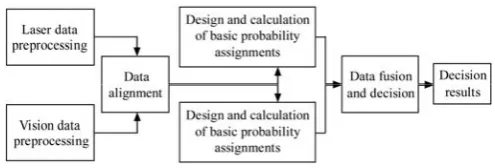
Considering some uncertainties, such as false detection and missing detection with whether laser radar or machine vision, and data redundancy due to the detection of the same tree trunk by the two sensors, Dempster-Shafer theory was chosen to deal with those uncertainties and redundancy. The fusion process is shown in Figure 1. Firstly, some preprocessing works were implemented, such as single calibration of laser radar and vision camera, reduction of measurement noises of laser data and preprocessing of vision data. Then, data alignment was implemented by the combined calibration from the laser coordinate system to the image coordinate system. Subsequently, basic probability assignment functions with a frame of discernment were designed rationally and calculated for regions of interesting (RoIs) of laser data and vision data respectively. At last, data fusion was conducted in light of evidence combination rules and decision should be made in light of decision rules of Dempster-Shafer theory.
Figure 1 Decision level fusion based on Dempster-Shafer theory 2.2 Preprocessing of sensors data
Several preparations were carried out before data fusion. First of all, time synchronization was conducted to acquire for the two sensors by using the same computer. Then, the two sensors were calibrated respectively. Here camera calibration was achieved using the Matlab Camera Calibration Toolbox, and laser calibration was carried out to detect the installed error and the measurement error[19]. Then, the raw data from the two sensors
were preprocessed.
In theory, the precision of laser radar is high, but a lot of noises usually are contained in laser data due to its systematic errors, reflection or transmission of some measured objects, mixed pixel and ambient light, which reduce the measure precision of laser radar. Here, median filter with three neighborhoods was adopted to process the data to reduce the effect of measurement noises.
A 2D linear interpolation method was used to preprocess images from the vision sensor to reduce the range of data hole. The method is to search four closest pixels around an interpolating pixel point. Then, the gray value of the interpolating pixel point was obtained by weighed average of the four pixels gray values, where the reciprocal of distance was set as the weight. This method is simple with fast speed processing.
2.3 Data alignment between sensors data
Data alignment between laser and vision sensors was carried out to implement data fusion, because they have different data representation and different resolution. Here, a combined calibration based method was used to solve the problem of data alignment between the two sensors.
For a camera sensor, the 3D world coordinates are transformed to the 2D image coordinates, and there is only one corresponding pixel in an image for one point in the 3D space. Also, each data point from a laser sensor has a unique position in the 3D world coordinate system. Thus for one laser data point, there is only one corresponding point in the 3D world coordinate system, and also there is only one corresponding point in the image. Therefore, the calibration can be implemented from the laser coordinate system to the image coordinate system, considering the fact that it is plane scanning for laser radar and its scanning points are located on the calibration plane.
2.3.1 Single line laser radar model
The 3D coordinates of any radar data point P can be expressed by the following Equation (1) in the world coordinate system (Figure 2).
1 1
P
p P
p P
X x
Y
M y
Z
⎡ ⎤ ⎡ ⎤
⎢ ⎥ ⎢ ⎥
⎢ ⎥ = ⋅ ⎢ ⎥
⎢ ⎥ ⎢ ⎥
⎢ ⎥ ⎣ ⎦
⎢ ⎥
⎣ ⎦
(1)
where, [XP,YP,ZP,1]T is the homogeneous coordinate of the point P
in the Cartesian coordinate system; [xP,yP,1]T is the homogeneous
Figure 2 2D laser sensor model 2.3.2 Camera model
For a camera sensor, the 3D world coordinates are transformed to the 2D image coordinates, as shown in Figure 3. Any point P= [XP,YP,ZP]T in the world coordinate system has the only projection
point p=[u,v]T in the 2D image plane W, and O is the center of
projection.
Figure 3 Camera model This perspective projection can be expressed as:
1
1 P P
P X u
Y
λ v Q Z
⎡ ⎤
⎡ ⎤ ⎢ ⎥
⎢ ⎥= ⋅⎢ ⎥
⎢ ⎥ ⎢ ⎥
⎢ ⎥ ⎢ ⎥
⎣ ⎦ ⎢ ⎥
⎣ ⎦
(2)
where, [u,v,1]T is the homogeneous coordinate of the projection
point p in the image plane W; [XP,YP,ZP,1]T is the homogeneous
coordinate of the point P in world coordinate system; λ is a scaling factor; Q is a 3×4 perspective projection matrix, which is determined by the internal and external parameters of the camera. 2.3.3 Direct calibration method of laser radar and camera
According to Equations (1) and (2), the transformation is obtained from the laser coordinate system to the image coordinates system as Equation (3), where G is a 3×3 conversion matrix.
1 1 1
P P P P
x x
u
λ v Q M y G y
⎡ ⎤ ⎡ ⎤
⎡ ⎤
⎢ ⎥ ⎢ ⎥
⎢ ⎥ = ⋅ ⋅⎢ ⎥= ⋅⎢ ⎥
⎢ ⎥
⎢ ⎥ ⎢ ⎥
⎢ ⎥
⎣ ⎦ ⎣ ⎦ ⎣ ⎦
(3)
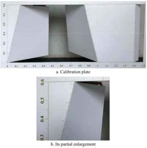
The traditional solution to the conversion matrix G is to implement the two calibration process respectively to calculate the rotation matrix M and the perspective projection matrix Q. But the disadvantage of this method is that every calibration will introduce error and thus it will result in a greater error for the calculation of the conversion matrix G due to error accumulation. To find the image pixel points corresponding to the laser data points, a rectangle calibration plate is adopted as shown in Figure 4, which is referred to the literature [20]. The plate has two inward concave regions (Figure 4a), one is on the left with isosceles trapezoid, and another is on the right with rectangular. And positions of all vertices of the two regions can be measured accurately in the plate coordinate system. The plate coordinate system OBxByB is connected to the plate, the origin point of the
coordinate system is set on the bottom left corner of the isosceles trapezoid, the xB axis is horizontal to the right, and the axis yB is
vertical to the up. Figure 4b is the partial enlargement of the
calibration plate with scaling marks, and the scaling marks can be positioned with visual interpretation.
There are certain differences for the laser scanning data reflected from the inward concave regions and the flat part on the plate. According to these differences and the geometric relationship, the coordinates of some special laser scanning points in the calibration plate can be calculated, and then the corresponding positions in the image found according to the coordinates of the special scanning points in the plate coordinate system.
a. Calibration plate
b. Its partial enlargement
Figure 4 Calibration plate and its partial enlargement 2.3.4 Combined calibration algorithm of laser and image
The model of the calibration plate was established as shown in Figure 5, where the sold lines represent the edge of the inward concave regions, and the dotted line indicates the position of the scanning line. The three intersection points A, B and C between the laser scanning line and the two waists of the trapezoid and the left edge of the rectangular are regarded as the special points. Thus, the coordinates of these special points are calculated respectively in the laser coordinate system and the image coordinate system. Then, the conversion matrix G of Equation (3) was calculated in light of the obtained coordinates of these special points above.
Figure 5 Plate model
From Figure 5, the linear equations of two waists of the isosceles trapezoid were y=4x and y=-4x+4 in the calibration plate. And the coordinates of A, B and C points can be expressed as:
The length of line segment of AB and BC were lAB and lBC
respectively, and the following equations can be obtained according to the distance equation between two points.
2 2 2
(xA−xB) +(4xA+4xB−4) =lAB (4)
2 2 2
(1.4−xB) +(yC+4xB−4) =lBC (5) And the following equation can be obtained according to the collinear condition of A, B and C points.
4 4 4 4 4
1.4 A B C B
A B B
x x y x
x x x
+ − = + −
− − (6) Thus, the coordinates of A, B and C points can be calculated according to Equations (4)-(6). Then, the coordinates of the three special points in the image plane are calculated in light of the exact coordinate scales in the calibration plate, thus to realize the matching of laser data points and image pixels.
A set of calibration data {(x1,y1,u1,v1), (x2,y2,u2,v2), …,
(xn,yn,un,vn)} can be achieved by changing the position of the
calibration plate in front of an agricultural vehicle with a camera and a laser radar, as the agricultural vehicle is kept stationary.
Set a transition matrix G:
11 12 13
21 22 23
31 32 33
g g g
G g g g
g g g
⎡ ⎤ ⎢ ⎥ = ⎢ ⎥ ⎢ ⎥ ⎣ ⎦ (7)
Substitute G in Equation (3), then we have:
11 12 13
21 22 23
31 32 33
1 1
p p x
g g g
u
λ v g g g y
g g g
⎡ ⎤ ⎡ ⎤ ⎡ ⎤ ⎢ ⎥ ⎢ ⎥ ⎢ ⎥ =⎢ ⎥⋅ ⎢ ⎥ ⎢ ⎥ ⎢ ⎥ ⎢ ⎥ ⎢ ⎥ ⎣ ⎦ ⎣ ⎦ ⎣ ⎦ (8)
Eliminate λ, then we have:
31 32 33 11 12 13
31 32 33 21 22 23
( )
( )
P P P P
P P P P
u g x g y g g x g y g
v g x g y g g x g y g
⋅ + ⋅ + = ⋅ + ⋅ +
⎧
⎨ ⋅ + ⋅ + = ⋅ + ⋅ +
⎩ (9)
By Equation (9), each set of laser-image data pairs can determine two equations, so at least 5 sets of data pairs are needed to solve the matrix G. Here the value of g11 is set to 1, and
Equation (9) is converted to:
12 13 31 32 33
21 22 23 31 32 33
( )
( ) 0
P P P P
P P P P
g y g u g x g y g x
g x g y g v g x g y g
⋅ + − ⋅ + ⋅ + = −
⎧
⎨ ⋅ + ⋅ + − ⋅ + ⋅ + =
⎩ (10)
Usually, n>5 is selected to reduce the calibration error, and then 2n equations can be obtained as n sets of data pairs are substituted to Equation (11). Set X=[g12, g13, g21, g22, g23, g31, g32,
g33]T, the 2n equations can be rewritten as:
1 1 1 1 1 1
1 1 1 1 1 1 1
1 0 0 0 0 0 1
1 0 0 0 0 0 1
n n n n n n n n n n n n n
y u x u y u
x y v x v y v
y u x u y u
x y v x v y v
− ⋅ − ⋅ − ⎡ ⎤ ⎢ − ⋅ − ⋅ − ⎥ ⎢ ⎥ ⎢ ⎥ ⎢ − ⋅ − ⋅ − ⎥ ⎢ ⎥ ⎢ − ⋅ − ⋅ − ⎥ ⎣ ⎦ # 1 0 0 n x X x − ⎡ ⎤ ⎢ ⎥ ⎢ ⎥ ⎢ ⎥ ⋅ = ⎢− ⎥ ⎢ ⎥ ⎢ ⎥ ⎣ ⎦
# (11)
The matrix G can be calculated when the equations above are solved by using the least square method.
2.4 Data fusion and decision based on Dempster-Shafer theory 2.4.1 Concept of basic probability assignments
For tree detection in an orchard environment, a frame of discernment is defined as Ω={T, NT}, where T refers to the tree trunk, and NT indicates not the tree trunk. So, a nonempty set of the frame Ω includes three subsets of {T}, {NT} and {T, NT}. A function m:2Ω→[0,1] is called a basic probability assignment if it
satisfies m(Φ)=0, where Φ is empty set, and ( ) 1 A Ω
m A ⊆
=
∑
The quantity m(A) is defined as A’s basic probability number. It represents the strength of some evidence.
2.4.2 Basic probability assignments of laser data
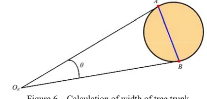
The information of trunk width is chosen as evidence to design the basic probability assignments of laser data preprocessed by median filter. Considering the fact that a tree trunk is approximately cylindrical and the distance from radar to the tree trunk is so farther than the diameter of the tree trunk, the polar radius values of all laser data points corresponding to the tree trunk are very close, and the edge of the tree trunk can be detected in light of the change rate of polar radius, as shown in Figure 6, where the point OR represents the original point of laser radar, the lines
ORA and ORB represents the polar radius values of the edge of tree
trunk, θ is intersection angle of the lines ORA and ORB, AB
represents the width of the trunks. According to the relative triangle Equations, we have
2 2 2 2 cos
R R R R
AB =O A +O B − ⋅O A O B⋅ ⋅ θ (12) According to Equations (12), the trunks width can be calculated. Here, the calculated width of the tree trunk should be smaller than the tree trunk diameter, but they are very close.
Figure 6 Calculation of width of tree trunk
Assuming that the limit of the trunk width is W=[wmin, wmax],
where unit is millimeter, and when the diameter of one measurement is di, the basic probability assignment of laser data
points indicating the tree trunk is:
min
max
1 min max
( )/10
1 1 min
( )/10
1 max
if [ Δ , Δ ]
( ) if Δ
if Δ
i i
i w w Δw
i w Δw w
i
k w w w w w
m T k e w w w
k e w w w
− −
+ −
∈ − +
⎧ ⎪
=⎨ ⋅ < −
⎪ ⋅ > +
⎩
(13)
where, k1 is a constant and general close to 1; m1(T) is the belief
level that the data points represent the tree trunk, the greater value of m1(T) means that the data points represent the tree trunk with the
greater likelihood; Δw is the measurement error of the tree trunk. Also, assuming m1(Ω)=0, thus m1(NT)=1-m1(T), where m1 (NT)
means the likelihood of laser data points is not a tree trunk. 2.4.3 Basic probability assignments of vision data
After preprocessing with a 2D linear interpolation for data hole, the tree image includes three parts, i.e., the regions of green plants such as tree leaves and weeds, tree trunks and big branches, and background region mainly composed of soil. Here a stripping segmentation algorithm is proposed to strip out the regions not belonging to tree trunk regions part by part, as shown in Figure 7. The algorithm was detailed with examples in Section 3.2.2.
Assuming that the matching level of the corresponding vision points of the tree trunk is α, α∈[0,1], which value is determined by calculating width and height of consecutive pixel points (possible tree trunk) in the stripped image after the feature extraction of tree trunks. The higher the matching level α is, the higher the similarity level of tree trunks. Here, we define
2( ) 2 0 1
2
1 0.8 1 (Ω)
0.1 0 0.8
α α
m α
α −
⎧ ≤ ≤
⎪ = ⎨
⎪ ≤ <
⎩
(15)
where, k2 is a constant and general close to 1. Thus, m2(NT) =1–
m2(T)–m2(Ω), which means the likelihood that the vision points are
not tree trunks.
Figure 7 Algorithm of stripping segmentation 2.4.4 Data fusion and decision
For a frame of discernment Ω, m(*) indicates the basic probability assignment using the evidence combination of Dempster-Shafer theory[21], as shown in Equation (16).
1 2
1 2
1 2
( ) ( )
( ) ( )
1
( ) ( )
X Y Z
X Y Φ
m X m Y
m Z m m Z
K
K m X m Y
∩ =
∩ =
×
= ⊕ =
−
= ×
∑
∑
(16)After the evidence combination, decision will be made based on the basic probability assignment[21], then we have:
1
2
( ) ( )
(Ω) ( ) (Ω)
m T m NT ε
m ε
m T m
− >
⎧
⎪ <
⎨
⎪ >
⎩
(17)
where, T is the decision result; ε1 and ε2 are the preset threshold
values.
In Equation (17), the first inequality indicates that it should keep sufficiently large difference for each evidence to support all the different propositions, otherwise, it is thought that this evidence does not inclined to support certain proposition. The second inequality means the uncertainty level for the objective proposition, and when the uncertainty level of the evidence is very large, it is not sufficient for the evidence of sensors to classify targets. The third inequality represents that it cannot classify when the knowledge of a target is poorly little.
3 Experiments and analysis
3.1 Combined calibration tests of laser sensor and vision camera
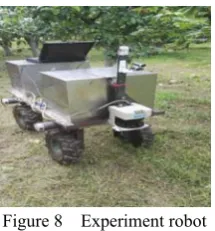
The tests were conducted in an agricultural robot, where a SICK LMS 192 laser scanner with a scanning distance of 8 meter, and a scanning angle of 180º and an angular resolution of 0.5º, was fixed on the front of the robot body with tiny downward sloping; a web camera of PK-910H with 1280×720 pixels resolution and about 60° angle of view, was fixed with a downward angle of 15°; A laptop computer TL-N12 was used to acquire and process sensor information, as shown in Figure 8. The calibration plate was vertically placed in the robot front, and 7 sets of laser-image data pairs were obtained with 7 different location of the plate, but it should be always guaranteed that the scanning line of the laser radar sweeps the two waists of the isosceles trapezoid and the rectangular edge in the plate and the plate must be in the camera view.
Figure 8 Experiment robot
According to one set of laser-image data pairs, the coordinates of the special points of A, B and C (Figure 5) were determined in the laser coordinate system, and the length of the line segment AB and BC were calculated. Then, these points were located in the image and their coordinates were obtained in the image coordinate system. Thus the matching of laser data and image pixels were implemented. The calculation process above was repeated to solve the special points of the calibration plate at different positions in front of the agricultural robot, and thus 14 sets of calibration data was obtained as followed (the units are m and pixel respectively):
M={(0.1956, 2.235, 365, 361), (0.4234, 1.91, 451, 341),…, (–0.7788, 2.199, 68, 357)}.
There are four elements in one subset, where the first two elements are the coordinates in the laser coordinate system, and the last two elements are the coordinates in the image coordinate system.
According to Equation (11), the conversion matrix G was calculated:
1 0.5230 0.1437 0.0094 0.2385 0.4905 0.0002 0.0016 0.0002 G
−
⎡ ⎤
⎢ ⎥
= ⎢ ⎥
⎢ − ⎥
⎣ ⎦
The laser data points were projected onto the image according to the conversion matrix G, as shown in Figure 9. The red points indicate the position of the scanning points of the laser in the image coordinate system after calibrating.
Figure 9 Results of the linear fitting
3.2 Field experiments 3.2.1 Experiments design
Field experiments were conducted in a pear orchard at the horticultural experiment field of Nanjing Agricultural University, on the same platform mentioned above (Figure 8). The robot was located on different position along pear trees rows, and the computer acquired sensors data in time. The 40 images and laser data were acquired from 9:00 am to 10:00 am and form 2:00 pm to 3:00 pm in sunny day and cloud day respectively. And the measurement for tree trunk width was conducted for 120 trees by using laser sensor. Then tree trunks were detected according to data pairs from laser radar and camera.
3.2.2 Image processing and matching level calculation
tree trunks were stripped out, as shown in Figure 10. Considering that there are almost green canopy of trees on the upper of an image (1280×720 pixels, Figure 10a), we selected local region of the image (1280×540 pixels, Figure 10b), which can accelerate the speed of image processing. After preprocessing data hole and analyzing the 40 images, we found the RGB values of trunks are all less than 200, the values of blue color are almost less than the values of green color and one of the RGB values of soil background is always less than 50, so we segmented the local
region image and obtained a gray image, as shown in Figure 10c. After binaryzing, a binaryzation image was shown in Figure 10d. Then, morphological operations such as “fill, open and close” were conducted for further image processing, as shown in Figure 10e, where the remaining RoIs were labeled. At last, feature extraction of tree trunks was performed in light of the fact that the height of tree trunks is bigger than the width in images, so we obtained Figure 10f where the RoIs with labels of 1, 4, 5, 8 and 9 were remained.
a. Raw image b. Local image c. Gray image
d. Binarized image e. Image after morphological operations f. Extraction with labels Figure 10 Image processing
The following equation was applied to calculate the matching level αof tree trunks:
α=min{1, k3·AB/ABB} (18)
where, AB indicates the area of a labeled region; ABB indicates the
area of the bounding box for every labeled region, which is the smallest rectangle containing the labeled region, as shown in Figure 10f; and k3 is a constant, here set k3=2. Therefore, α values of
matching level are 0.64, 0.36, 0.66, 1 and 0.52 for the labeled regions 1, 4, 5, 8 and 9 in Figure 10f respectively. Here, the matching level αof the labeled region 5 is larger than those of the labeled regions 1, 4 and 9 corresponding to tree trunks.
3.2.3 Tree trunk width measurement
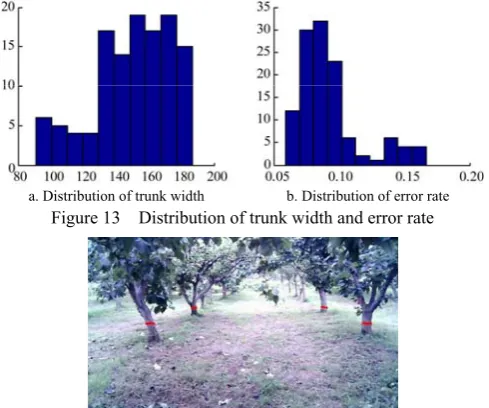
According to laser data like Figure 11, which corresponds to the scene of Figure 10a, the trunk width was calculated by Equations (12). The measured values of trunk width of 120 trees were compared to true values of tree trunk width, as shown in Figures 12 and 13. The values of trunk width are mainly at 130-185 mm (Figure 13a), but the measured values are all not more than the true values, which error rates are limited at 6%-16.7%, and mainly at 7% and 10% (Figure 13b). For Figure 11, the trunk width values for labels of A, B, C and D are 0.1836, 0.1696, 0.1735 and 0.1806, respectively. It should be noted that we only considered laser data points from 60º to 120º due to about 60º angles of view of the web camera used here.
Figure 11 Laser data
Figure 12 Width of tree trunks and error rate of trunk width 3.2.4 Data fusion and decision
The laser data points were projected onto the tree image according to the conversion matrix G in Figure 14. The red points indicate the position of the scanning points of the laser in the image coordinate system after calibrating.
a. Distribution of trunk width b. Distribution of error rate Figure 13 Distribution of trunk width and error rate
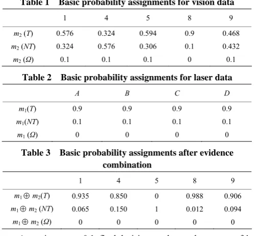
data were calculated by Equation (14). And the basic probability assignments of the labeled regions of 1, 4, 5, 8 and 9 were 0.576, 0.324, 0.594, 0.9 and 0.468 in Figure 10f respectively at k2=0.9.
Table 1 and Table 2 showed the basic probability assignments of the label A, B, C, D and 1, 4, 5, 8, 9 for a frame of discernment Ω including {T}, {NT}and {T, NT}. From data pairs of laser sensor and vision sensor, the label A, B, C and D in Figure 11 corresponds to the label 9, 8, 4 and 1 in Figure 10f, respectively, but no data from laser sensor corresponds to the label 5. Therefore, we defined the corresponding basic probability assignment as m(T)=0, and m(NT)=1.
Evidence combination was conducted according to Equation (16), the results is shown in Table 3.
Table 1 Basic probability assignments for vision data
1 4 5 8 9
m2 (T) 0.576 0.324 0.594 0.9 0.468
m2 (NT) 0.324 0.576 0.306 0.1 0.432
m2 (Ω) 0.1 0.1 0.1 0 0.1
Table 2 Basic probability assignments for laser data
A B C D
m1(T) 0.9 0.9 0.9 0.9
m1(NT) 0.1 0.1 0.1 0.1
m1 (Ω) 0 0 0 0
Table 3 Basic probability assignments after evidence combination
1 4 5 8 9
m1⊕m2(T) 0.935 0.850 0 0.988 0.906
m1⊕m2 (NT) 0.065 0.150 1 0.012 0.094
m1⊕m2 (Ω) 0 0 0 0 0
Assuming ε1=ε2=0.1, final decision results are that targets of 1,
4, 8 and 9 are tree trunks according to Equation (17), but target 5 is not, although it has high matching level like tree trunk.
4 Conclusions
A novel algorithm based on data fusion of a vision camera and a 2D laser scanner was developed to detect tree trunks accurately in forestry and fruit farming. The data fusion is achieved through the integration of decision level with Dempster-Shafer theory. A calibration plate with two inward concave regions was used to implement data alignment between two sensors data. Tree trunk width measurement by laser radar and image processing by a stripping segmentation algorithm were performed to determine basic probability assignments of RoIs for two sensor data respectively.
A robot platform was used to acquire data from sensors and to perform the presented tree trunk detection algorithm. Experiments were conducted in a real pear orchard under sunny and cloudy conditions. Results showed the algorithm was successful to detect tree trunks and data fusion improved tree trunk detection ability. This algorithm can provide a new method for tree trunk detection and accurate production and management in orchards.
Acknowledgments
The study was supported by “Jiangsu Provincial Natural Science Foundation of China (No. BK20151436) and Blue Project of Jiangsu Province”.
[References]
[1] Gertsis A, Fountas D, Arpasanu I, Michaloudis M. Precision agriculture applications in a high density olive grove adapted for mechanical harvesting in Greece. Procedia Technology, 2013; 8(3): 152–156. [2] Berk P, Hocevar M, Stajnko D, Belsak A. Development of alternative
plant protection product application techniques in orchards, based on measurement sensing systems: A review. Computers and Electronics in Agriculture, 2016; 124: 273–288.
[3] Sanz R, Rosell J R, Llorens J, Gil E, Planas S. Relationship between tree row LiDAR-volume and leaf area density for fruit orchards and vineyards obtained with a LiDAR 3D dynamic measurement system. Agricultural and Forest Meteorology, 2013; 171-172(3): 153–162.
[4] Ježová J, Mertens L, Lambot S. Ground-penetrating radar for observing tree trunks and other cylindrical objects. Construction and Building Materials, 2016; 123: 214–225.
[5] Juman M A, Wong Y W, Rajkumar R K, Goh L J. A novel tree trunk detection method for oil-palm plantation navigation. Computers and Electronics in Agriculture, 2016; 128: 172–180.
[6] Kan J M, Li W B, Sun R S. Automatic measurement of trunk and branch diameter of standing trees based on computer vision. Proceedings of 3rd IEEE Conference on Industrial Electronics and Applications, 3-5 June, 2008; pp.995–998.
[7] Liang X, Litkey P, Hyyppä J, Kaartinen H, Kukko A, Holopainen M. Automatic plot-wise tree location mapping using single-scan terrestrial laser scanning. The Photogrammetric Journal of Finland, 2011; 22(19): 37–48.
[8] Lehtomäki M, Jaakkola A, Hyyppä J, Kukko A, Kaartinen H. Detection of vertical pole-like objects in a road environment using vehicle - based laser scanning data. Remote Sensing, 2010; 2(3): 641–664.
[9] Rahman M Z A, Gorte B. Tree filtering for high density airborne LiDAR data. International Conference on LiDAR Applications in Forest Assessment and Invertory, Edinburgh, UK, 2008.
[10] Bargoti S, Underwood J P, Nieto J I, Sukkarieh S. A pipeline for trunk localisation using LiDAR in trellis structured orchards. Field and Service Robotics, Switzerland: Springer International, 2015.
[11] Hamner B, Singh S, Bergerman M. Improving orchard efficiency with autonomous utility vehicles. 2010 ASABE Annual International Meeting, Pittsburgh, PA, USA, 2010.
[12] Guivant J, Masson F, Nebot E. Simultaneous localization and map building using natural features and absolute information. Robotics and Autonomous Systems, 2002; 40(2-3): 79–90.
[13] Zhang J, Chambers A, Maeta S, Bergerman M, Singh S. 3D perception for accurate row following: methodology and results. 2013 IEEE/RSJ International Conference on Intelligent Robots and Systems, Tokyo, Japan, 2013.
[14] Ali W, Georgsson F, Hellstrom T. Visual tree detection for autonomous navigation in forest environment. 2008 IEEE Intelligent Vehicles Symposium, Eindhoven, Netherlands, 2008.
[15] He B, Liu G, Ji Y, Si Y, Gao R. Auto recognition of navigation path for harvest robot based on machine vision. International Conference on Computer and Computing Technologies in Agriculture IV. Springer Berlin Heidelberg, 2011.
[16] Morgenroth J, Gomez C. Assessment of tree structure using a 3D image analysis technique - a proof of concept. Urban Forestry and Urban Greening, 2014; 13(1): 198–203.
[17] Cheein F A, Steiner G, Paina G P, Carelli R. Optimized EIF-SLAM algorithm for precision agriculture mapping based on stems detection. Computers and Electronics in Agriculture, 2011; 78(2): 195–207. [18] Shalal N, Low T, Mccarthy C, Hancock N. Orchard mapping and mobile
robot localisation using on-board camera and laser scanner data fusion – part B: mapping and localisation. Computers and Electronics in Agriculture, 2015; 119(Supp. 2): 267–278.
[19] Zhang S S. Navigation of an agricultural autonomous vehicle based on laser radar. MS dissertation. Nanjing: Nanjing Agricultural University, 2014; 6. 25p. (in Chinese)
[20] Liu D X. A research on LADAR-vision fusion and its application in cross-country autonomous navigation vehicle. Changsha: National University of Defense Technology, 2009; 2. 44p. (in Chinese)