The Reduced Rules Rule Based Forecasting Decision Support System: Details and Functionalities: An Audit Context

The Reduced Rules Rule Based Forecasting Decision Support System:

Details and Functionalities: An Audit Context

Manuel Bern1 & Edward Lusk2 1

TUI AG, Hannover, Germany 2

State University of New York (SUNY) at Plattsburgh, 101 Broad St., Plattsburgh, NY, USA & Department of Statistics: The Wharton School: University of Pennsylvania, Phila. PA, USA

Correspondence: E. Lusk, SBE SUNY Plattsburgh, 101 Broad St. Plattsburgh, NY, USA 12901.

Received: June 15, 2020 Accepted: July 12, 2020 Online Published: July 20, 2020 doi:10.5430/afr.v9n3p13 URL: https://doi.org/10.5430/afr.v9n3p13

Abstract

In execution of PCAOB audits at the Planning and Substantive Phases, forecasts of various financial account balances are often used to collect information on the veracity of the client‘s final reported balances. One of the forecast methods widely acclaimed in the academic context is the Rule Based Forecasting [RBF] model of Collopy and Armstrong [C&A]. However, for the most part, the RBF has not found its way into the panoply of the auditor. In our practice-oriented experiential context, the reason for this seems to be the lack of an enabling Decision Support System [DSS] usually needed to create reliable RBF-forecasts in a timely manner needed at the Substantive Phase of the audit. Focus In this report, we detail a GUI-friendly DSS, the VBA-programming of which is based upon a 2013 revision of an updated C&A model offered by Adya and Lusk. The DSS is called: The Reduced Rules: Rule Based Forecasting: Decision Support System [RR:RBF:DSS]. We provide a comprehensive example of the RR:RBF:DSS in a PCAOB-audit context for a Caterpillar™, Inc account Panel downloaded from Bloomberg™. This example, carefully details all of the numerous User Form-Launch platforms as well as discusses the statistical and operational Rule-scoring functionalities of the RR:RBF:DSS. The RR:RBF:DSS is available as a download without cost or restrictions on its use.

Keywords: analytical procedures, PCAOB JEL: M42 O43

1. Introduction 1.1 Overview & Context

The Reduced Rules Rule Based Forecasting Decision Support System [RR:RBF:DSS] is based on the work of Adya & Lusk (2013) [A&L] The link to A&L is: [https://www.irjaf.com/previous-issues.html][Month-link:August 2013(note 1); the full text is found on: Vol.13:Pages(1006:1024). It is strongly recommended that you read A&L before using the RR:RBF:DSS. In this report, we will discuss the development of Rule Based Forecasting from its initial launch by Collopy & Armstrong (1992) [C&A] to the RR:RBF:DSS presented in this paper. It will benefit the reader to understand these developmental points of evolution to enrich the understanding of how to maximize the beneficial use of the RR:RBF:DSS.

1.2 Report Presentation Specifically, we will present:

1. The developmental linage of RBF from C&A to the RR:RBF:DSS detailed in this report,

2. The nature of the information processing commitment required in using the RR:RBF:DSS in the Audit-context. Following we will use InCharge to indicate the individual responsible for conducting the audit OR the members of the audit team engaged in the Planning and Substantive Phases of the PCAOB-audit,

4. A detailed illustrative forecast produced in the Audit & Assurance context for a PCAOB Audit. The dataset is that of Caterpillar™ Inc. as taken from the Bloomberg™ Terminal Link: SUNY:Plattsburgh, USA, and

5. The Conclusion and Outlook for extensions of this research. 2. Lineage of RR:RBF:DSS

To better understand the DSS offered in this report it would be productive to examine the developmental precedents upon which the RR:RBF:DSS is based.

2.1 The Core Concepts Offered by Collopy and Armstrong

The world of forecasting was delivered a rude-awaking in 1982. Prof, Spyros Makridakis and a number of forecasting luminaries published the results of a forecasting competition: called the M-Competition where: a 1001 economic time series were collected and analyzed re: the forecasting acuity of a plethora of en vogue forecasting models of the day. Prof. Makridakis reasoned: here, liberally stylistically paraphrasing Armstrong et al. (1983):

There is a glut of forecasting models. The time has come to see which of the horses are the best in

the stable.

This produced the first M-competition the details of which are found in Makridakis et al. (1982). The results were indeed surprising—actually, they shocked the forecasting world. What emerged as the ―Best in the Time-Series Class‖ among the 30 some models tested were: four models. The standard OLS two-parameter [Intercept & Slope] Linear model dating from the work of Karl Pearson (1857-1936), Sir Francis Galton (1822-1911) and Sir R.A Fisher (1890 -1962) [OLSR], The Holt/ARIMA(0,2,2) Model: (Holt (1957[2004]); a two parameter exponential smoothing model dating from the mid-1950s[Holt], Brown‘s linear exponential smoothing model Brown (1959), and remarkably: The Naïve I model, which uses the last confirmed observation as the forecast, outperformed many of the more elegant mathematical and statistical models! These M-competition results were the motivation of C&A who selected 126 time series from the M-Competition to develop their groundbreaking forecasting model called: Rule Based Forecasting-Expert System model [RBF]. C&A examined the peer-reviewed literature to extract forecast modeling strategies that were therein reported, conducted a survey of 49 Experts in the forecasting-milieu to determine what factors and forces affect the accuracy of forecasting extrapolations, and taped interviews taken with five forecasting experts who described guidelines that they employed to create useful forecasts. In the C&A study, two critical sets of forecasting definitions were offered:

2.1.1 Appendix A: Definition of the Features

These 18 features were coalesced from the copious intel collected from the experts, the C&A Appendix A had three sub-sections:

(i) Identified by Rules [Eight Concepts]: For example: Direction of the Recent Trend. The direction of the trend that results from fitting Holt’s model to the historical data,

(ii) Input by the Analyst based on Inspection of the Data [Six Concepts]. For example: Suspicious Pattern: Series that show a marked changes in the recent pattern, and

(iii) Input by the Analyst based upon Domain knowledge. [Four Concepts] For example: Cycles Present: Regular movement of the series about the Trend.

2.1.2 Appendix B The Rule Base The RBF model had 99-RBF-Rules

The first ten[10] Rules addressed Adjusting the Historical Data and Identification Features—for example: Rule [1] Truncation: IF there are irrelevant data early data, THEN delete these data. [Prior data are relevant for extrapolation only if the underlying process is stable]. The remaining 89 RBF-Rules when found to be TRUE produce shifting weights given among the four core RBF-Models. For example, for the Short-Range Model Level Rule [30] Near Extreme IF the last observation is near a previous extreme AND the series has cycles present THEN subtract 10% of the weight on the random walk [Naïve I] and add it to that on the regression and on Brown’s. {When the last observation is near a previous extreme it may be there due to chance or to transient factors. There may also be a bound on the series. Accordingly, less emphasis is given to the latest observation.}

2.2 Overview of the RR:RBF:DSS

As elegant and important as the C&A RBF model is, it has a ―chink in its armor‖. In the practical forecasting context: ―Time is of the Essence.‖ To expect the harried forecaster to devote due diligence to mixing and matching: The 18 Features and 99-Rules over Four Models—well, requires a challenging leap-of-faith in the statistical expertise, mathematical training, and time available to the forecaster whose ―forecasts are needed—usually ‗Yesterday‘ ‖. Adya & Lusk (2012). For this reason, Adya acting on the final advice of C&A (p.1408):

The rule-based forecasting procedure offers promise. We provide our rules as a starting point. Hopefully, they will be replaced by simpler and fewer rules.

offered the next developments and refinements to the C&A RBF version. Circa 2000 Adya and her colleagues corrected, simplified and automated the initial C&A RBF expert system. See: [Adya (2000); Adya, Collopy, Armstrong & Kennedy (2000); Adya, Collopy, Armstrong & Kennedy (2001). These considerable refinements fine-tuned the C&A RBF model; we refer to the ―final‖ version as: RBF[2000]. The next evolution was effected by A&L (2013). Based upon eight years of testing in academic settings, A&L taught and tested various RBF[2000] versions with an eye to continue to evolve the RBF[2000] model to ―Simplify and Reduce‖ the Rules of the RBF expert system. This lead to the research report: A&L (2013): Reduced Rules Rule Based Forecasting—where there are 12 weight-modification rules, three blending Rules C&A[97, 98 & 99], and 7 features. The A&L lean-model is termed: The Reduced Rules Rule Based Forecasting [RR:RBF] model.

However, in our discussions with various individuals engaged in forecasting, we gleaned that the ―Time to Forecast‖ still seemed to be an impediment to the use of: (i) the RBF[2000] version or, interestingly and surprisingly, (ii) the A&L RR:RBF-versions. Therefore, the next obvious developmental evolution was to create a system of processing platforms to reduce the Time to Forecast—to wit: a DSS. Perhaps, we reasoned, such a decision-aid, would stimulate use of the extraordinary ground breaking work of C&A and its leaner progeny: the RR:RBF:DSS.

Following we will detail various aspects of the RR:RBF:DSS. The RR:RBF:DSS is programmed in Excel™ using open-VBA™ modules and is offered free with NO restrictions on it use—academically or commercially(note 2). 3. The Nature of DSS: RR:RBF:DSS or Otherwise

In its essence, the RR:RBF:DSS is ONLY a decision AID or SUPPORT tool. The reason we are mentioning this will be best articulated by the following personal-vignette:

―A young student did very poorly on a third-grade Spelling Test. At the evening dinner, the parents mentioned quizzically: ―You certainly did not do well on your Spelling test, did you?‖ The child, with conversational candor, quipped: ―Well, what do you expect, the stupid Pen could not Spell—I ask you! What was I to DO?‖

One of the problems identified and reinforced by our experience is that users of forecasting Decision Support Systems [DSS] have come to believe that such DSS are the present day: Oracles of Delphi—the infallible voice of what the future holds. This is, of course, as fallacious and ludicrous as the Pen that could not Spell.

The morale is: Responsibility and Accountability lie with the User not the Tool. In this spirit, consistent with Adya & Lusk (2012), we have organized the RR:RBF:DSS to be highly interactive. As mentioned above the DSS-design imperative was to engender: Commitment and Responsibility through Goal-Seeking Engaged Technological-Interaction. The nature of this required engaged-interaction is a reinforcement of the ―Tool‖ nature of the RR:RBF:DSS. To be more specific, the RR:RBF:DSS engages the InCharge through queries so as to move along in the modular execution of the RR:RBF:DSS; these queries are an important feature of the RR:RBF:DSS, the intention of which is to engender a commitment of ―Ownership and also Accountability‖ in the forecasts generated from the interaction of the decision-maker with the RR:RBF:DSS of: Bern & Lusk(2020). However, we do recognize that engendered engagement may work at cross-purposes with the ―Time to Forecast‖ imperative that seems to ―rule‖ in the forecasting domain. Perhaps, our design context of required engagement will be an impediment to the use of the RR:RBF:DSS. We will address this possible conundrum in the Outlook section of this report.

4. Overview of the Essentialities of the RR:RBF:DSS

4.1 Features Selected From C&A

There are 28 features in the C&A version. We have selected from this collection the following: 1. Irrelevant Early Data

2. The Nature of the Causal Forces

3. Direction of the Basic Trend. Sign of the Regression Slope/Trend 4. Direction of the Recent Trend. Sign of the Holt Slope/Trend 5. Changing Basic and Recent Trend

6. Significance of the OLSR: Basic Trend

7. Recent Run Long Test

8. Near a Previous Extreme

9. Outlier Screen: Box-Plot Calculation 10. Level Discontinuity or Level Shift

The bolded features are used in the A&L version; See Table 1 p.1023. The Italicized features are ―computations‖ that are used in conjunction with the bolded-features in executing the 12 Reduced Rules of A&L. All of these follow the letter of the features as discussed in C&A and so as adopted by A&L excepting the Outlier Screen. We have decided, after sample testing not presented herein, to use the more prevalent and code-friendly Box-Plot Whiskers-Model of Tukey[See SAS™.JMP™:v13:DiscriptiveAnalysis[BoxPlot]].

4.2 RR:RBF:DSS Protocol-Set

There are seven Worksheets [WSs] in the RR:RBF:DSS. So as to facilitate the understanding of the flow of the various modular protocols woven into the fabric of the RR:RBF:DSS, we will offer an brief overview of these seven WSs.

On opening the RR:RBF:DSS there is a VBA-Alert that offers the following advice: You have Opened the RR:RBF:DSS. BEFORE you use this Decision-Making Tool Please Open the WorkSheet called: READ ME FIRST. There you will find important information that will help you in creating information using the RR:RBF:DSS. WS[1]: ReadMeFirst The WS: ReadMeFirst essentially introduces the Tool nature of the RR:RBF:DSS the implication of which is that the InCharge must be engaged in the process of using this Tool to aid in the creation of RBFs.

WS[2]: GeneratingProcesses This is a detailed discussion of Additive and Multiplicative processes. In the C&A versions, it is recommended that if the process generating the data in the Panel is Multiplicative that the [log or ln]-transformation be taken and the transformed Panel be used in forming the RBFs and then re-transformed back to the original units. This WS argues that this transformation protocol is fraught with analytic difficulty and is to be avoided. In fact, A&L did not use transformations in their refinement of the RBF[2000].

WS[3]: IndexOfRR RBF DSS this is a brief overview of the various WSs in the DSS.

WS[4]: RegressionDataFixer Sometimes in downloads there are Missing Data or Data values that are ―Contextually Anomalous‖. WS[4] offers functionalities to Fill the Panel for the Missing data points and also to substitute values for the Anomalous data as identified in the Download. These data-filling-protocols are: VBA-coded, very simple, and not used in the Enders (2010) Sense of Missing Data Analysis that usually require ―reference data or variable sets‖ to form the fill values.

WS[5]: Profiles This is where the ten A&L-Features noted above are developed from the Data Panel as modified by the RegressionDataFixer. These feature profiles will be used by the InCharge to score the 12-RR:RBF rules that will be used to form the final RR:RBFs.

WS[7]:SampledData These are a random sample of dataset from the first M-competition. They were used by C&A and also A&L in developing and testing various aspect of the final RBF & RR:RBF:DSS. These were used over a multi-years testing frame both in the USA, Europe, and China.

4.3 The Functional Nature of the RR:RBF: Pre-Analysis Phase

Before the creation of the Profile of the Dataset, the first issue to be addressed by the InCharge is to make a reasoned selection of data to be used in the RR:RBF:DSS. This falls under 1. Irrelevant Early Data. In addressing the quality of the selected data panel to be forecasted there are two issues that should be considered: (i) Irrelevant Early Data, and (ii) Subsumed in this rubric is the Event-Space Anomaly.

4.3.1 Irrelevant Early Data

It is sometimes the case that the generating function changes over time. Such evolutionary morphing is normal—sometimes called the learning-curve. For example, the nature of the generating process for start-ups changes as the organization moves into a more mature/stable phase of operations. In this case, it is wise to exclude data generated in the start-up phase as it does not contribute to understanding the short-term future of the organization.

4.3.2 Event Anomalies

In addition to start-up data that is basically endogenous to all firms after the firm leaves the start-up phase, the next issue is determining if there are Event Anomalies in the ―Life-Panel‖ of the firm that will be used in forecasting. Usually, these are exogenous to the organization—simply, events outside the organization happen in the economic context that affect the firm. For example, the September 2008 melt-down of Lehman Bros™. LLP sent an economic shock--a kin to the Black-Friday of the 1929 US stock-market crash through the world economy. Additionally, the COVID-19 pandemic has created an event-horizon that may rival Lehman for its devastating economic impact. Schneeweiss, Murtaugh, Atkinson & Rathi (2020, p.50) note: The most optimistic scenario is still bad. Therefore, it is recommended that the InCharge considers the Start-Up [Endogenous Anomalies] and Event [Exogenous Anomalies] in selecting the Panel to be forecasted. The next basic issue is to consider the Causal Forces.

4.3.3 Causal Forces Identification

We recommend that before the InCharge looks at a plot of the data or produces the Features of the Panel to be forecasted that the InCharge reflects as to the possible nature of the Causal Forces. To make relevant, and so useful, forecasts, it is necessary to understand the context of the forecasting task. This follows in a natural way as many of the facettes or issues regarding the Causal Factors or Forces were likely considered in forming a Panel that was ―free‖ from Endogenous & Exogenous Anomalies. C&A define Causal Forces as those aspects of the organization that influence the generating forces of the data—basically Causal Forces are endogenous to the organizational milieu. Specifically, C&A [p.1409] note: Causal forces are ―the net directional effects of the principal factors acting on the series‖; these are the factors that are or affect the generating functions of the output of which are the measured points in the Panel. Specifically, there are five offered by C&A: ― „Growth’ exerts an upward force at all times. ‘Decay’ exerts a downward force at all times. ‘Supporting’ forces push in the direction of the historical trend. ‘Opposing’ forces work against the trend. Finally, ‘Regressing’ forces exert pressure towards a mean.‖ C&A offer the wise advice that: ―Forces should only be specified when they are obvious; otherwise, they should be identified as ‘Unknown’ ‖. In this context, we suggest for the forecaster not to observe a Plot of the data or its Summary Feature-Profile and then make up a reason to select one of the Causal Forces; this seems to be necessary if the InCharge wishes to avoid a "Data-Anchoring" issue—the tendency to write a story that fits the data sample that may be very different from the ―population‖ story. Experience teaches that this may lead to a bias where there are judgments required in the forecasting model. To be clear, in the majority of our forecasting exercises both as a consultant and in an academic setting, we score Causal Forces as: Unknown.

Assuming that the analyst has selected a reasonably representative ―error‖ free-Panel —i.e., not perturbed by an Event-Anomalies—and Scored the Causal Forces, then the next phase is engage the various functionalities of the RR:RBF:DSS.

4.4 The RR:RBF:DSS Worksheet Platforms

4.4.1 The Regression Fixer: WS[4]

This is the first data creation panel or Worksheet to be used in the RR:RBF:DSS. After the reflections re: the Event and Causal Issues, this next phase is data-driven and is intended to fine-tune the Panel. Protocol: Place the Selected Panel into Col[A] of the WS[4]:RegressionDataFixer. This platform is to be used ONLY IF there are e-download issues. In our experience, not infrequently, there is missing data or data that is manifestly unlikely due to the downloading process. In this case, we have created an analysis platform for modifying the selected Panel-dataset so that it can be better used in the forecasting context. WS[4] has nothing to do with outlier analysis; using WS[4] we address modifying the downloaded data for clear data-errors or missing-data. Outliers are NOT errors; they are part of the variability of the data. Experience and the literature strongly advises to correct errors but to leave "outliers" in the dataset. Also this is our advice. Experiential context: Download issues using Bloomberg terminals are rare. However, in the CRSP™ & COMPUSTAT™ massive-download milieu, we have experienced download issues about 2% of the time.

WS[4]RegressionDataFixer offers are two ―data-fixes‖ that are sometimes needed where there are Missing or Anomalous Data points. A TextBox that informs the InCharge follows:

Data Fixer DSS: This RR:RBF:DSS platform is used to fix data sets using 'Unobtrusive" Blending and Replacement methods. First, click Clear to remove all previous data and formatting. Then, paste the data set into Col[A] (DO NOT paste over the title in A1) Next, click the Blank button to fill-in any missing data points. This will launch a UserForm with three different options to choose from for filling empty cells: {Average : Median : Blend}. The Blend is the Nearest Neighbor Average. IF there are NO Missing Values, click any of the three options and the full dataset will be forwarded to Col[B] the next checking phase: The Anomalous Phase. Then, click the Anomalous button to replace any Anomalous data points using:{Average : Median : Blend}replacements. Specifically, the Anomalous button replaces data points that are outside the three times the BoxPlot multiplier as scripted:

LowerLimit = 25thPercentile(B:B)  [3×(1.5) × [IQR] UpperLimit = 75thPercentile(B:B) + [3 × (1.5) × [IQR]]

Alert The Blank & Anomalous buttons are only to correct obvious download glitches. Interestingly, in a download-browser context, data-values sometimes are "missing", impossible, or highly improbable and so need to be replaced in the forecasting context. These glitches are not outliers; outliers will be considered in the WS:Profiles values that occur more than infrequently. 4.4.2 The Feature Profile presented WS[5]

Profiles To aid the InCharge in better understanding the time series under examination, we have created a Features Worksheet in the RR:RBF:DSS. Following is the set of InCharge-guidelines that is generated by the RR:RBF:DSS in the WS[5]:Profiles. Protocol: After the WS[4]RegressionDataFixer, the InCharge will move to the Features profiling phase where most of the information usually needed to guide the InCharge will be produced in WS[5]. The DataSet is pasted in Col[A] of WS[5] from the WS[4]:RegressionDataFixer. Then an OLS two-parameter linear regression [OLSR] is run using the Excel: DataAnalysis[Regression] platform. The Regression values generated by the OLSR are match-pasted in Col[C]. The Panel-Series is Point by Point [i] de-Trended as: Col[D(i)] = [Col[A(i)]  Col[C(i)]]. In Col[E(i)] is the change value over the Panel: specifically, Col[E(i)] = [Col[A(i)]  Col[A(i+1)]]. Then the following Feature related parameters are presented:

F1: Direction of the Basic Trend: Sign/Magnitude of the OLSR slope: IF > 0, then ―Positive‖ ElseIF < 0, then ―Negative, last: ―Slope Equals Zero‖. Point of Information: The OLSR is a Time Series forecasting Excel-platform. Therefore, for RR:RBF:DSS to function it must be run using the Microsoft™ Suite where: Add-ins: [Analysis ToolPak-VBA and the Analysis ToolPak] are both enabled. There are no intellectual property rights infringements if one has purchased the Microsoft Suite.

independently from the RR:RBF:DSS. In our developmental work where the RR:RBF:DSS was programmed and tested we used the SAS™[JMP™[v.10/12/13]] which has the Holt model. However, we elected not to integrate SAS[JMP] into the RR:RBF:DSS as this would require all users to also purchase the Holt-Link through SAS. In our discussions with possible users, the clear recommendation was to leave the Holt decision to the user. If possible users have another Holt: software version then it would be unreasonable for them to purchase the SAS-link just for the RR:RBF:DSS when in fact they could simply integrate their Holt software into a RR:RBF:DSS VBA-platform. In this report, we will be using our version of SAS[JMP.13[TimeSeries[Holt]]].

F3 Basic Trend Significant Here we upgraded the C&A rule that uses as the measure of significance [Abs[t], of the OLSR-slope >2.0]; we used the reported OLSR-slope p-value and the Excel code: IF(p-value> 0.05,"NonSignificant","Significant").

F4 Near a Previous Extreme Here the rule-set of C&A [p.1409] lacks a few conditional specifications. We have taken the liberty to create a codex that fulfills the spirit of the ―Near a Previous Extreme Screen‖. We offer: If the last observation: O[n] of the Point by Point de-trended series is: [> 90% of the Max[Point]] OR [< 110% of the Min[Point]] provided that the previous extreme observation: O[n-1] is NOT the one immediately preceding the last one[O[n]], then Near a Previous extreme is recorded. We simplified this to first evaluate if the last observation [O[n]] is IN the following C&A-implied Capture Interval:

[LowerLimit[LL]: [UpperLimit[UL]] [[110% of the Min[Point] : [90% of the Max[Point]]

The Excel codex that is used for this feature is:

Codex: {IF(AND(O[n]>=LL,O[n]<=UL),"NotNearPreviousExtreme",_ IF(OR(O[n-1]<LL,O[n-1]>UL),"NotNearPreviousExtreme","NearPreviousExtreme"))}

F5 Recent Run NOT Long According to C&A and A&L, if the period to period movement for the last six observations have not all been in the same direction then Recent Run Not Long is scored as TRUE. There is a VBA screen that evaluated the last six panel points for the five sign changes. If there are any cases where the signs are all not the same then Recent Run Not Long is scored as TRUE.

F6 Outliers Here we have modified the protocol for the detection of outliers and also the decision action that is recommended. The reason for this is that in C&A the 95%CI is not specified. There are, in fact, three such 95%CIs: Excel, Fixed Effects and Random Effect versions. These have been detailed and discussed in Bern and Lusk (2020). For this reason, and also as we do not advise modifying outliers in the Panel, we are using the relatively standard Tukey: Box-Plot to screen for outliers. This is basically the same coding that we used for the Anomalous screen of WS[4]:RegressionDataFixer. However, in this case, we are using the Actual Tukey-Whisker Boundaries which are the default in the SAS[JMP.v13]:

LowerWhiskerLimit = 25thPercentile(B:B)  [(1.5) × [IQR] UpperWhiskerLimit = 75thPercentile(B:B) + [(1.5) × [IQR]]

This outlier screen is VBA-coded and reports individually the number of Low and High outlier points in the dataset. Our experience in the forecasting context is that removing outliers can unrealistically mollify the inherent variation of the series. Therefore, we have created a Rule Impact screen to be sensitive to the outlier profile of the Time Series. Our experience, suggests that if number of outliers in the Panel is more than 20% of the points in the Panel, then this often suggests an instability consistent with the fact that the Causal Forces are Unknown.

The Excel-Codex is: IF((Low + High)/COUNT(A:A)>20%,"There is likely an INSTABILITY in the DataSet. This often rationalizes the Decision that the Causal Forces are Unknown. The Rules to consider are: RULES {40, 41, 76, 77, 97, 98 & 99}. ","Owing to the Lack of Outliers, the Series seems relatively stable. This often rationalizes the Decision that the Causal Forces are Known")

Summary Advice: The InCharge should use the Outlier Platform to calibrate their judgmental confidence in making the decision scoring of the various rules. To be clear, we do NOT support altering the dataset for outliers and re-creating the profile of the dataset.

profiles. This profiling is very important for the intelligent scoring of the 12 A&L Rules. The important implication is that although the WS[5]:Profile takes less than 1-minute to create the information, the InCharge should carefully reflect on the meaning of this profiling info-set so as to score the RR:RBF Rules with confidence born of careful judgmental reflection. We recommend that the InCharge discusses the output of WS[5] and that of the RR:RBF-Rule scoring logic. Our trials with students, in classroom setting, suggest that most groups were able to arrive at a set of scored-rules from their interactive dialogue in 90 minutes or so. Once the InCharge is satisfied that they have gleaned the insights sufficient to score the 12-RR:RBF-Rules, then WS[6]RulesScoring will be used to this end.

At this point, we offer an example. In the context of this research report, it will NOT be possible to detail all the computations that are involved; actually, this is not necessary as they are scripted out in the A&L research report. Additionally, we recommend that the reader access the DSS: URL(note 3) and download the RR:RBF:DSS so as to follow along with the information presented in the illustrative example.

5. Example Caterpillar™, Inc. [CAT] 5.1 PCAOB Context

It is clear that there is a ―first-mover‖ advantage in having accurate forecasts that guide the ERP&C platforms of the organization. Therefore, to expand and enrich the ―scope‖ impact of the RR:RBF:DSS, we have adopted an assurance PCAOB engagement as the illustration. The first version of the RR:RBF model was tested in the Audit context for one of the ―Big Four‖ Audit & Assurance LLPs in Frankfurt[Main], Germany. However, due to the propriety nature of the data collected in that audit context, we have used an illustrative Panel taken from the Bloomberg™ Terminals(note 4). Additionally, this CAT dataset is also proprietary information; therefore, we are not permitted to give the actual data identified by Account and Time-period. However, we are permitted to use the numbers not specially identified by context. The context assumed for this illustration is the PCAOB Assurance Audit for Caterpillar, Inc. [CAT:NYSE] SEC[SIC:3531]:FY-ending 31Decs. The InCharge is using the recommended Analytic Procedures protocol at the Planning Phase to forecast, at the Substantive Phase, the Client‘s closing quarter ending: Q13: [31Dec]. This testing of the AP-phase is required by the PCAOB [AS5[Dec2017]. See Gaber & Lusk(2017). The Quarterly [Q] forecasting Panel is presented in Table 1.

Table 1. Account [Bloomberg[FA:CAT:GAAP:Highlights:Millions of USD].

Qs Q1 Q2 Q3 Q4 Q5 Q6

Value $9574 $9822 $11 331 $11 413 $12 896 $12 859

Qs Q7 Q8 Q9 Q10 Q11 Q12

Value $14 011 $13 510 $14 342 $13 466 $14 432 $12 758

The InCharge is using the RR:RBF:DSS to create the AP-Audit Forecast for the YE-Q 20xx[Q13] Value. This will then be compared to the actual value for the closing quarter Q13: as closed for the client‘s AIS. This comparison is then used to rationalize if Expended Procedures for the Account for CAT are warranted. The actual value for YE-Q 20xx[Q13] is $13 144.00

To illustrate the RR:RBF:DSS, we give a running commentary—including the time spent—for the various platforms that are used to arrive at the final RR:RBF:DSS forecast.

5.2 Basic Illustrative Data Panel

We selected Caterpillar as it is a PCAOB Audit[CAT:NYSE] and does not seem to have any Audit Issues over the Panel. Specifically, (i) using EDGAR™: For CAT[20xx & 20xy] there were no trading suspensions(note 5) nor |delinquent filings(note 6), and (ii) using WRDS™[AuditAnalytics™[AA] Database, there were only: Is Effective 305 designations. Further, there were no required 10-K re-fillings made during the Panel period. Also CAT was listed and actively traded during the Panel time period. Using the Bloomberg Terminals, we downloaded all of the 10-K filings and there were no Qualified or Adverse Audit reports that were not scope related. Finally, we searched the BBT:[ICS[CAT:CompanyNews[KeyThemes]] platform for 20xx & 20xy; we found no indications that there were issues that would have made CAT an atypical illustrative example. This was the phase of the RR:RBF:DSS where Irrelevant Early Data and Event-Anomalies are used as a filter to select a ―qualified‖ Panel for forecasting. Time {2h35 Mins; this information was also used in the Causal Forces analysis presented subsequently.}

smoothed as a yearly panel that would have folded back beyond 10 years that could tacitly have created a Lehman-Event anomaly.

Following, we will illustrate, in reasonable detail, the RR:RBF:DSS and indicated all the steps that one of the co-authors used in arriving at the final RR:RBF for the Caterpillar Panel[Q1 to Q12] to produce a RR:RBF for [Q13].

5.3 The RR:RBF:DSS: In Execution: The Causal Forces Imperative

First, we pasted the CAT dataset into ColA of the WS:RegessionDataFixer. The indication was that were no Missing nor Anomalous data points in the CAT-Panel. This is consistent with the information from EDGAR, WRDS[AA] & the Bloomberg Terminals discussed above. Next, we considered the forecasting task at hand in the PCAOB-CAT-Audit context so as to form an opinion as to the Nature of the Causal Forces. In this regard, we were guided by the Generally Accepted Audit Standard [GAAS] of the AICPA(note 7) [PCAOB&SEC]. Specifically, the following Second Standard of Field Work[SFW[2]] provided excellent guidance in contexting the Analytic Procedures aspect of the CAT-audit and also offers homomorphic council to forming a reasonable opinion as to the Causal Forces:

GAAS[Standard of FieldWork[2]]

The auditor must obtain a sufficient understanding of the entity and its environment,

including its internal control, to assess the risk of material misstatement of the financial statements whether due to error or fraud, and to design the nature, timing, and extent of further audit procedures.

The required due diligence to satisfy GAAS:SFW[2] will require that we, ―the CAT-InCharge‖, who will be using the RR:RBF:DSS, form a detailed understanding of the prevailing and expected Causal Forces.

5.3.1 The Relational Pre-analysis for Forming an Opinion of the Causal Forces for the CAT-Assurance Audit In this regard, we formed a relational Pearson Product Moment Correlation [PPMC] set to judge the ―Stability of Total Revenue with other Impact Variables in the Market Trading Context‖. This is presented in Table 2

Table 2. PPMC Associations with Selected Sensitive CAT: Accounts

Account as Correlated PPMC

Operating Income 0.91*

Net Income to Common 0.60

Basic EPS, GAAP 0.61

Cash and Equivalents 0.24 Total Current Assets[CA] 0.91 Total Current Liabilities[CL] 0.53 Current Ratio [CA/CL] 0.77

Average 0.65

* Bolded values are greater than the Harman Screening Factor[(.5)^.5]

The correlation table suggests that Account is in sync with the expected related Accounting Variables; this confirms the EDGAR, BBTs & WRDS[AA] profiling as discussed above. Finally, we downloaded the Analysts Reports [ANRs] from the BBTs. The Analyst reports and recommendations were mixed: Buy or Hold or Sell; no clear theme was identified. Overall for the Panel period the Percentages of Buy: Hold: Sell were very constant at {40% : 50% : 10%} a strong profile suggesting a stable and well managed firm. Implication Caterpillar is well managed and in tune with the economics of the revenue generating processes of their industry group. However, this is merely the back-drop for labelling the Causal Forces.

5.3.2 Causal Forces Coding

Caterpillar is very active in the global markets, in particular, in China where there are strong indications that a massive infusion of earth moving and construction equipment will be needed in the near-future as China moves to address its energy short-fall by adding nuclear power to its electricity grid. However, circa the end of the Panel, there are serious likely possible impediments to realizing the benefits of an active and long-term economic engagement in China due to ―trade-war‖ issues between the USA & the PRC. After a GoogleChrome™ search [URL](note 8), we found confirmatory information circa September 2019 of problematic economic issues between CAT and China. Specifically, we could not determine, circa September 2019, with convincing certainty, what could be the likely effect of the possible trade ―war‖ issues between the USA and China. We could see that Causal Forces re: CAT could be Decaying or could be Growing relative previous global activity depending on the nature of the future ―hard-line‖ posturing or easements or conciliations between the USA & China. True, Caterpillar is very well managed and stable firm BUT it appeared to us that they are caught-up in a maelstrom of political uncertainty over which they do not likely have any control. For this reason, relative to the short run activity circa the YE-quarter 20xx, we scored the Nature of the Causal Forces as Unknown.

5.4 The RR:RBF:DSS Engaged

In this case, we will now move to the data generating phases of the RR:RBF:DSS. Recall that we have serviced the due-diligence needed—specifically, in executing WS[4]:RegressionDataFixer the Panel was deemed: not corrupted by Missing or Anomalous data, and the Causal Forces analytics we well developed leading to the decision that the Causal Forces are Unknown. This pre-analysis then rationalizes moving to the data generating phase of the RR:RBF:DSS.

5.4.1 Profiling Phase

In this case, the RR:RBF:DSS passed the CAT-Panel to the WS[5]:Profile. In this WS, first we used our SAS[JMP.v13] software to compute the Holt parameters(note 9). In this regard,

The Holt Level was: 14 095.86, and

The Trend was: -666.80.

Further, the graphical profile produced was:

Figure 1. Panel Values for Caterpillar [Ticker CAT] Inc

Regarding the various profiles as discussed above, we found the following all of which were produced by the RR:RBF:DSS:

•Direction of the Basic Trend: Positive [The OLSR: Slope was +381.46] •Direction of the Recent Trend: Negative [The Holt: Slope was: -666.80 •Basic Trend Significant: TRUE: p-value= <0.001.

•Near Previous Extreme: TRUE: The C&A interval was: [-1095.52 : 1157.19] In this case, the Last trend adjust value was: O(n):-1874.54 and its neighbor point was: O(n-1):180.92. In this case, the last observation was outside of the C&A interval while the neighbor point was in the C&A interval; thus, the last point was Near a Previous Extreme.

•Recent Run Long: FALSE over the last six points[7:12] there were three relative decreases and two related increases.

•Outlier Check using the Tukey Box Plot: None were identified as the CAT[Whisker Interval] was: 8028.38 : 16 999.38 and there are NO Panel values not in this CAT[Whisker Interval]

0 10000 20000

1 2 3 4 5 6 7 8 9 10 11 12

CAT:Series

5.4.2 The Rules Scoring

Using this Profile-Intel, we then launched the Rule Scoring Platform: WS[6]:RuleScoring For this platform the following parameter set was populated:

Table 3. The Level and Trend Values as inputted and created by the RR:RBF:DSS

RR:RBF Values Level Trend

RW 12 758.00 0.00

OLS 14 632.54 381.46

Holt 14 095.86 -666.80

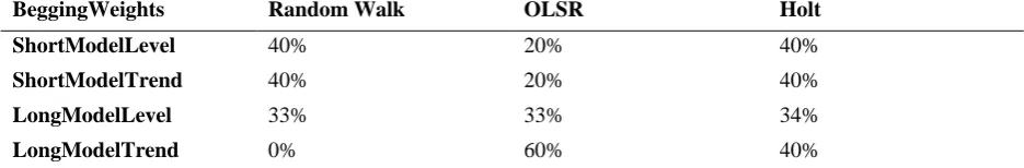
Further, the Starting A&L weighting Values are:

Table 4. The Initial Starting Weights for the four RBF Disaggregated Models

BeggingWeights Random Walk OLSR Holt

ShortModelLevel 40% 20% 40%

ShortModelTrend 40% 20% 40%

LongModelLevel 33% 33% 34%

LongModelTrend 0% 60% 40%

Each of the 12-A&L RR:RBF Rules will be presented in turn and noted as they are scripted in A&L. Recall and recognize that the RR:RBF:DSS is aiding the Decision-process rather than making the decisions for the InCharge. The 12-Rules with respect to the four model forms are distributed over the four RR:RBF components as follows:

{Short Model Level Adjustments: A&LRules {29 & 32}, {Short Model Trend Adjustments: A&LRules {40, 41 & 42},

{Long Model Level Adjustments: A&LRules {67 &71}, {Long Model Trend Adjustments: A&LRules {76, 77, 78, 86 & 87}

The next set of queries are for the 12 Rules are in the A&L Appendix. Each one is produced in the order of the A&L presentation; actually in C&A and so in A&L there is NO order effect in the scoring of the 12 Rules(note 10). We will present our scoring and a brief justification. At the end of the Rule scoring we will give the final weights after all the weights are modified that can be compared to the A&L Starting Weights in Table 4.

Short Model Level

Rules 29/67: Level Discontinuities (Short Model Level) IF there is a level discontinuity, THEN 10% will be added to the Random Walk Level and 10% will be subtracted from the Holt Model Level. If NOT, then NO CHANGE is recorded. Scored [FALSE]: [There were no level Discontinues observed in the CAT Panel as found on the Plot of the CAT-Panel. No weight modification. 2 Mins]

Rules 32/71: Changing Recent Trend (Short Model Level) IF there is an unstable Recent Trend, THEN add 45% to the Random Walk Level and subtract 15% from the Linear Regression and subtract 30% from the Holt Model Level Weights. If NOT, then NO CHANGE is recorded. Scored [True]: [There was evidence of a Trend instability in that there were three positive changes and two negative changes using the C&A measure. We felt this non-cyclical “Wiggle” was consistent with an instability—not profound but certainly suggestive in the CAT Panel. Weight modification. 5 Mins]

Short Model Trend

above; the ongoing political trade-war posturing between President Trump & China suggested to us that there is reasonable uncertainty re: the duration of a Trade War that would affect the economic climate for CAT. For this reason, we scored Causal Forces as Unknown. 10 Mins]

Rule 41/77: Dissonance (Short Model Trend) IF the direction of the Recent Trend and the direction of the Basic Trend are not the same, OR if the Trends agree with one another but differ from the Causal Forces, THEN add 15% to the Random Walk Trend and subtract 5% from the Linear Regression Trend and subtract 10% from the Holt Model Trend Weights. If NOT then NO CHANGE is recorded. Scored[TRUE]: [The Trend of the Holt was Negative [-666.80] while the Basic Trend [OLS-Regression] was Positive [381.46]; also the Basic Trend was significant. Therefore, we scored this as TRUE and thus the weights were modified. 10 Mins]

Rule 42/78: Inconsistent Trends (Short Model Trend) IF the direction of the Basic Trend and the direction of the Recent Trend are not the same, AND the Basic Trend is not changing, THEN add 20% to the Linear Regression Trend and subtract 20% from Holt Model Trend. If NOT, then NO CHANGE is recorded. Scored[False]: [The Trend of the Holt was Negative [-666.80] while the Basic Trend [OLS-Regression] was Positive [381.46]; also the Basic Trend was significant. However, we scored Rule 32 as True in that it appeared that the recent trend was not stable. Thus as there is an AND condition for this rule re: the stability of the Recent trend we scored this Rule as False. 7 Mins]

Long Model Level

Rule 67/29: Level Discontinuities (Short Model Level) IF there is a level discontinuity, THEN 10% will be added to Random Walk Level and 10% will be subtracted from the weight of the Holt Model Level. If NOT, then NO CHANGE is recorded. Scored[FALSE]: [See Rule 29. 1 Min] Rule 71/32: Changing Recent Trends (Long Model Level) IF there is an unstable Recent Trend, THEN add 63% to the Random Walk Level and subtract 21% from the Linear Regression Level and subtract 42% from the Holt Model Level Weights. If NOT, then NO CHANGE is recorded. Scored[True]: [See Rule 32] There was evidence of a Recent Trend instability in the CAT Panel. 1 Min]

Long Model Trend

Rule 76/40: Causal Forces Unknown (Long Model Trend) IF the Causal Forces are unknown, THEN add 10% to the Random Walk Model Trend and subtract 10% from the Linear Regression Trend. If NOT, then NO CHANGE is recorded. Scored[TRUE]: [See Rule 40. 1 Min]

Rule 77/41: Dissonance (Long Model Trend) IF the direction of the Recent Trend and the direction of the Basic Trend are not the same, OR if the Trends agree with one another but differ from the Causal Forces, THEN add 15% to the Random Walk Trend and subtract 5% from the Linear Regression and 10% from the Holt Model Trend Weights. If NOT, then NO CHANGE is recorded. Scored[TRUE]: [See Rule 41. 1 Min]

Rule 86: Inconsistent Trends (Long Model Trend) IF the directions of the Recent and Basic Trends are not the same, THEN subtract 10% from the weight on Linear Regression Trend and add 3.3% to the Holt Model Trend and add 6.7% to the Random Walk Model Trend Weights. If NOT, then NO CHANGE is recorded. Scored[TRUE]: [The Trend of the Holt was Negative [-666.80] while the Basic Trend [OLS-Regression] was Positive [381.46]; also the Basic Trend was significant, 5 Mins]

Rule 87: Changing Basic Trend (Long Model Trend) IF there is a changing Basic Trend, THEN add 24% to the Random Walk Trend and add 6% to the Holt Model Trend Weights and subtract 30% from the Linear Regression Trend. If NOT, then NO CHANGE is recorded. Scored[FALSE]: [There was no evidence that the Basic Trend was changing in direction or materially in magnitude. 1 Min].

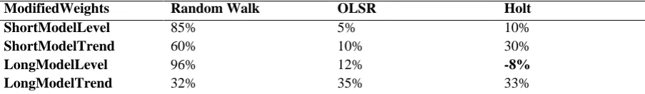
After we have scored these 12-Rules, there is a validity check that is part of the RR:RBF:DSS feedback loop. The feedback is predicated on the logic of the Rule-links. There are five Rule-Pairs that should logically be scored as the same. For example, IF Rule 29 is scored as True, THEN logically Rule 67 should be scored TRUE. Therefore, for each of the Rule-Pairs {29&67 : 32&71 : 40&76 : 41&77 : 42&78}, if they are not scored the same on a pair-wise basis, then there is color coding that alerts the InCharge of this fact. NO CHANGE is required as there may be a scoring logic in play for the InCharge that would rationalize a differential scoring. The intention is ONLY to provide the Alert as feedback; in some cases, the InCharge may choose to re-score the flagged-relationship. For the CAT-example, the consistency screen did not flag any inconsistent Rule-Pairs scoring. After these rules are scored or re-scored, then RR:RBF:DSS VBA-code modified weighting matrix that started out as noted in Table 4 will be modified. For the CAT-example, after the rules are scored the modified RR:RBF-weights are presented in Table 5. Table 5. The RR:RBF Weighting Matrix after Scoring the 12-RR:RBF-Rules

ModifiedWeights Random Walk OLSR Holt

ShortModelLevel 85% 5% 10%

ShortModelTrend 60% 10% 30%

LongModelLevel 96% 12% -8%

LongModelTrend 32% 35% 33%

It is the case, in the C&A and the A&L versions, that negative values such as -8%, could occur. This is NOT an error but merely a re-distribution of the relative weights. Once this re-weighting is finalized, the RR:RBF:DSS produces and displays all of the intermediate stages for the series under examination. For the CAT forecasting experience, the next decision is to make the decision regarding the final blending.

5.4.3 Re-Assembling the RR:RBF Components The blending is weighting of the Short and Long linear model forms into a single linear model and that is used to produce the final RR:RBFs. The RR:RBF:DSS produces a VBA:UserForm offering the following three choices:

97. Standard Blend. IF the trends from the short-range and long-range models are in the same direction OR if the causal forces are unknown, THEN

( ) (

)

where Lh is the percentage of the long-range model used in forecasting horizon h, and B is the blend period. This may be re-cast more simply as:

( )

98. Quick Blend. IF the short-range model direction conflicts with the long-range model direction AND the causal force direction is the same as the long-range model, THEN set the share of the long-range model to:

∑

99. Slow Blend. IF the short-range model direction conflicts with the long-range model direction AND the causal force direction is the same as the short-range model, THEN set the share of the long-range model to:

∑ ∑

After the Blending decision is made then the final RR:RBFs are produced. This is also transparent, so that if the InCharge is interested to trace through the computational logistics they are available.

In the case of CAT, we selected Blending Rule 97 as the Causal forces have been scored as Not Known. Point of Information If the Causal forces are Not Known, then it is the case that Rules 98 & 99 are eliminated from consideration. The final RR:RBFs over the six forecasting horizons produced by the RR:RBF:DSS are presented in Table 6.

Table 6. The Final Blended RR:RBFs for Caterpillar, Inc.

Horizon Final RR:RBFs Caterpillar

1 12 823.62

2 12 667.93

3 12 536.62

4 12 429.86

5 12 347.60

6 12 289.51

5.4.4 Discussion of an ―Anchoring‖ Trompe-l’œil

These are the six final forecasts produced by the RR:RBF:DSS for the CAT-audit engagement. Actually, only one forecast for CAT was required—this is bolded in Table 6. This forecast is generated at the Planning Stage and then when Caterpillar closes the books 31Dec20xx, the Substantive Phase, the InCharge will compare the AIS-value at YE with the RR:RBF[H1]. This is one of the PCAOB ―protocols‖ for Analytic Procedures testing. However, in many of the test situations, those using the RR:RBF:DSS, following the C&A-model where the blending period suggested is six(note 11), produce six-one-period ahead forecasts. In debrief sessions, at the Leuphana Universität, Lüneberg, Germany, students seemed be in a ―confidence-comfort-zone‖ after viewing plots of their six-period projections relative to the actual Panel values; their debrief sentiment was that if the projections of the six-periods looked reasonably stable, they felt more confident about their RR:RBFs. To better understand this ―anchoring‖ perception, consider the plots in Figure 2 where the first six-Panel values are the last six CAT-Panel values and the last six values in Figure 2 are the RR:RBFs.

Figure 2. CAT Real Data[Points 1:6] and RR:RBFs[Points 7:12]

Thus, the students seemed to be using the relative “stability” of the six-projections, Points[7:12] compared to the actual Panel values[Points 1:6] to validate the credibility of their projections. As a point of information, this sort of ―comfort-zone‖ anchoring does NOT seem a reasonable way to validate the ―credibility of the forecasts‖. The final blending—i.e., the RR:RBFs produced by the RR:RBF:DSS—are very smoothed; this is due to the nature of the Blending-Rules. The final RBFs never exhibit the ―typical stochastic variation‖ that would be the case for actual generating processes.

$10,000 $12,000 $14,000 $16,000

1 2 3 4 5 6 7 8 9 10 11 12

6. The Intervals of Interest: Risk or Capture 6.1 Capturing the Essence of the Forecasts

The RR:RBF:DSS produces one-set of RR:RBFs. This is the typical case. However, there are many variations thereupon. Two useful variations are the Delphi Protocol and Statistical Profiling. For the Delphi model, the interested and informed individuals constitute a single group that will parametrize the RR:RBF:DSS. For example, assume that the number of individuals on the audit team is n = q, where: q is typically less than 10, and they participate as a group in forming the information-set that will be used to parametrize the RR:RBF:DSS. Thus, the Delphi model generates one set of forecasts produced by a collective of individuals. This is always an excellent way to form forecasts that will likely be accepted by the Delphi-collective. The other RR:RBF:DSS option, Statistical Profiling, is that all q-individuals use the RR:RBF:DSS; in the typical case, this generates [q × 6]-forecasts. Then these forecasting-sets can be summarized using the Mean or Median. This Statistical Profiling version has the very desirable benefit that two sets of confidence intervals can be formed: One for the Lower Limits and one for the Upper Limits for each of the six-projection horizons. We recommend the usual 95%CI on each of the Mean values of the six projections; or alternatively the Median can be used and contexted by some measure of the Inter-Quartile Range. The Delphi protocol is logical and in our experience is more typically used than Statistical Profiling. The Statistical Profiling has NOT been programed in the RR:RBF:DSS. As an alternative, we have programmed a protocol that can be used to generate intervals that may aid the InCharge to intelligently process the RR:RBF-profile set generated.

6.2 Risk and Capture Intervals

This leads naturally to the last phase of the RR:RBF:DSS where there is the possibility of creating ―context-intervals‖ that are critically important in creating an action plan at the Substantive Phase of the audit. Recall, the purpose of using the RR:RBF:DSS was to forecast the YE-Q13—i.e., the first forecasting horizon: H1 = 12 823.62 as bolded in Table 6. However, a forecast without a contextual interval is practically of little value. For this reason and also because there are no forecasting intervals that are part of the theoretical development of the C&A or the A&L versions, we have offered a way to develop an interval context for the RR:RBFs. These are NOT statistically derived (1-α)Confidence Intervals. Simply they are judgmental intervals or boundaries fixed by the InCharge to form a context for the forecasts.

6.2.1 Risk Intervals

percentage risk level for making the decision to effect an AP EP-Investigation. According to logic of this section: If the YE:Q13 is IN these two risk intervals, that would tacitly indicate that there are a defensible set of reasons or conditions that could be used judgmentally to defend the decision not to effect an EP-examination for the Account in question. Logic would then suggest that: If the YE:Q13 is NOT IN the two risk intervals, that would tacitly indicate that there are a defensible set of reasons or conditions that could be used judgmentally to defend the decision to effect an EP-examination for the Account in question. The other two conditions would need to be defended judgmentally by the InCharge.

6.2.2 Capture Intervals

In this case, it is assumed that the InCharge has collected numerous post-audit profiles for the various audit Risk Classes used over time. Using these past-datasets of RR:RBFs and the matched capture information created after the actual values became available, then the InCharge may simply use the forecasting profiles accumulate over time to form, for the various ―risk‖-levels, the Quality of the Risk Profiles, where: Quality is measure by the percentage of time that the risk intervals as judgmentally parameterized captured the Actual values. These are then a posteriori or experiential intervals. This is NOT unlike the Makridakis, Hibon, Lusk & Belhadjali (1987) MHLB research report where they analyzed the capture rates of the first M-competition. We will not provide a detailed discussion of this Capture protocol as: (i) it is best demonstrated by MHLB, and (ii) actually, at this point, we do NOT have a large accrued dataset to form statistically powerful Capture-Risk profiles for the CAT illustrative example.

However, it is productive to illustrate the two aspects of the Risk protocol: Absolute and Percentage that were calibrated as: Risk[$625 & 5%]. As a point of information, in the Leuphana student trial, the approximate range interval for the Capture version for the Percentage was: [2% to 15%]. We did not collect information on the Absolute variations.

This gives the following Risk Intervals for the first projection horizon:

Risk[Absolute[$625]]: $12 823.62: [$12 198.62 : $13 448.62] & Risk[Percentage[5%]]: $12 823.62: [$12 182.44 : $13 464.80] For example, the 5%-Risk Interval is: [[$12 823.62 × (1  5%)] to [$12 823.62 × (1 + 5%)]].

In this case, the actual holdback value of: YE[Q13] is $13 144.00 is interior to both intervals. Also interestingly, there is a non-engineered crossing point for this pair of parameters. Starting at the fourth horizon the precision of the Percentage-Calibration becomes smaller than that of the Absolute-Calibration. From our student experience, this seemed to be a vetting-point for the ―logic of their calibration‖. In this case, the InCharge would likely: (i) not further investigate the AIS-booked Total Account of CAT as booked at YE[Q13], and (ii) document all of the above information as produced by the RR:RBF:DSS in the CAT-20xx audit working papers that will eventually become the CAT-permanent file. The reason for the recording all of the above is that IF there is a challenge to the due-diligence of the audit for the FPE or the FNE risk then this Total Account investigation and the related Risk-inferences to NOT launch an EP-investigation would very likely pass the best practices screen of the PCAOB.

7. Summary & Outlook 7.1 Summary

We have offered the first DSS that embodies the spirit of the groundbreaking work of C&A. This was possible due to the work of A&L who ratchetted-down the number of C&A-Rules from over 100 to around 15. Also A&L did not recommend or ever use the Ln/Log transformations in their work on the RR:RBF:DSS. Their logic is presented in the WS:[3] GeneratingProcesses where we treat the logic of eschewing data transformations in the RR:RBF context. We wish to emphasize that the RR:RRB is just a tool to facilitate the creation of information. The RBF system of C&A is an expert system and we find it to be one of the best judgmental forecasting decision tools developed to date. An essential underpinning of the work of C&A is to require careful consideration of developing indications to give a reasoned ―context‖ for the domain into which the forecasts are addressed to form reasonable guidance. This was also the developmental context of the A&L research report and finally our work.

7.2 Outlook

It is our hope that the RR:RBF:DSS finds currency in the forecasting milieu and also in the academic area. We offer the same advice that C&A offered in 1992:

The rule-based forecasting procedure offers promise. We provide our rules as a starting

Yes, we offer the same hope re: The RR:RBF:DSS. After all, any DSS that remains unchanged and does not evolve is not worth its programming effort. If there are individuals interested in the RR:RBF:DSS, it is an open-access VBA-Module system available as download at no cost and there are no restrictions on its use commercially or academically. We hope that if the RR:RBF:DSS is used that information on the Risk and the Capture rates be collect and made available. The author for correspondence would be delighted to receive such information and to post the same on an all-access download site.

We mentioned the fact that the decision to require InCharge-engagement in the creating the RR:RBFs using the DSS may work to create a dysfunction given the ―desire‖ of forecasters to produce ―forecasts in a timely manner‖. We have used RR:RBF:DSS versions over a number of years in academic instruction and in actual practice. The time to producing the RR:RBFs using the DSS that we reported for the CAT experience was around 4 hours—most of which was gathering the Intel to score the rules. This is typical in our experience and also the experience of the students using the test versions of the RR:RBF:DSS. This being the case, any ―time-concerns‖ about using the RR:RBF:DSS to form RR:RBFs would seem to be allayed. Four hours to produce high quality state of the art RR:RBFs does not rise to any level of ―a compromise‖ in the Time to Forecast domain.

Acknowledgments Appreciation are due to: Mr. John Conners, Senior Vice President, Financial Counseling, West Coast Region, AYCO for his generous philanthropy which funded the establishment of the John and Diana Conners Finance Trading Lab at the State University of New York College at Plattsburgh and the Bloomberg Terminals that were instrumental in this research. Further thanks are due to: Prof. Dr. H. Wright, Boston University: Department of Mathematics and Statistics, Frank Heilig, Senior IT Risk Division Manager: Volkswagen, Wolfsburg, Germany, Dr. Monica Adya, Dean and Professor of Management, Rutgers University - Camden, School of Business for her significant intellectual contributions in the study of forecasting that guided our DSS developments, and the reviewers of Accounting & Finance Research for their careful reading, helpful comments, and suggestions.

References

Adya, M. (2000). Corrections to rule-based forecasting: Findings from a replication. International Journal of Forecasting, 16, 125-127. http://doi.org/10.1016/S0169-2070(99)00034-5

Adya, M., Collopy, F., Armstrong, J.S. & Kennedy, M. (2000). An application of rule-based forecasting to a situation lacking domain knowledge. International Journal of Forecasting, 16, 477-484. http://doi.org/10.1016/S0169-2070(00)00074-1

Adya, M., Collopy, F., Armstrong, J.S. & Kennedy, M. (2001). Automatic identification of time series features for rule-based forecasting. International Journal of Forecasting, 17, 143-157. http://doi.org/10.1016/S0169-2070(01)00079-6

Adya, M., Lusk, E. & Balhadjali, M. (2009). Decomposition as a complex skill acquisition strategy in management education: A case study in business forecasting. Decision Sciences Journal of Innovative Education, 7, 9-36. http://doi.org/10.1111/j.1540-4609.2008.00199.x

Adya, M. & Lusk, E. (2012). Designing Effective Forecasting Decision Support Systems: Aligning Task Complexity and Technology Support, in C. Jao, ed.: Decision Support Systems, ISBN: 978-953-51-0799-6, (InTech, DOI:

10.5772/51255). Available from:

http://www.intechopen.com/books/decision-support-systems_2012/designing-effectiveforecasting-decision-sup port-systems-aligning-task-complexity-and-technology-sup https://doi.org/10.5772/51255

Adya, M. & Lusk, E. (2013). Rule Based Forecasting [RBF]: Improving efficacy of judgmental forecasts using simplified expert rules. International Research Journal of Applied Finance, 8, 1006-1024.

Armstrong, J. S., Lusk, E. J., Gardner Jr., E. S., Geurts, M. D., Lopes, L. L., Markland, R. E., McLaughlin, R. L., Newbold, P., Pack, D. J., Andersen, A., Carbone, R., Fildes, R., Parzen, E., Newton, H. J., Winkler, R. L., & Makridakis, S. (1983). Commentary on the Makridakis Time Series Competition (M-Competition). Journal of Forecasting, 2, 259–311. https://doi.org/10.1002/for.3980020308

Bern, M. & Lusk, E. (2020). Software: Reduced Rules: Rule Based Forecasting: Decision Support System [RR:RBF:DSS]. Download Only(note 12).

Brown, R.G. (1959). Statistical Forecasting for Inventory Control. McGraw-Hill.

Enders, C. (2010). Applied Missing Data Analysis. Guilford Press. ISBN 978-1-60623-0

Gaber, M. & Lusk, E. (2017). Analytical Procedures Phase of PCAOB Audits: A Note of caution in selecting the forecasting model. Journal of Applied Finance and Accounting, 4, 76-84.http://doi.org/10.11114/afa.v4i1.2811

Holt, C. 1957). Forecasting trends and seasonal by exponentially weighted averages. Published Archive: Office of Naval Research Memorandum. [ONRM:52]. The archive access is rather difficult; for this reason due to the important nature of this work, ONRM[52] was reprinted as: Holt, C. (2004). Forecasting Trends and Seasonal by Exponentially Weighted Averages. International Journal of Forecasting, 20, 5–10. http://doi.org/10.1016/j.ijforecast.2003.09.015

Makridakis, S., Andersen, A., Carbone, R., Fildes, R., Hibon, M., Lewandowski, R., Newton, J., Parzen, E. & Winkler, R. (1982). The accuracy of extrapolation (time series) methods: Results of a forecasting competition. International Journal of Forecasting, 1, 111-153. http://doi.org/10.1002/for.3980010202

Makridakis, S., Hibon, M., Lusk, E. & Belhadjali, M. (1987). Confidence intervals: An empirical investigation of the series in the M-Competition. International Journal of Forecasting, 3, 489-508. http://doi.org/10.1016/0169-2070(87)90045-8

Schneeweiss, Z., Murtaugh, D., Atkinson, A. & Rathi, A. (2020). A Shocked Economy. Bloomberg Markets: The Fear Issue, 29, 50-55.

Notes

Notes 1. We have the Adya & Lusk (2013) PDF as archived by the IRJAF. If you would like this PDF, we would be happy to e-send it to you. Contact the corresponding author.

Note 2. The RR:RBF:DSS is based upon the doctoral dissertation of Dr. Bern [Forecasting Methods in Audit Analytical Procedures – Potential Improvements in the Process and the Case for eDSS-assisted coreRule-Based Forecasting , OVG, Magdeburg, Germany]For this version: Contact Dr. Bern: [email protected]].

Note 3. The link to the DSS that was used in the illustrations presented in this paper are found in the link noted in the Bern & Lusk (2020) citation.

Note 4. https://www.bloomberg.com/

Note 5. https://www.sec.gov/litigation/suspensions/suspensionsarchive/susparch2018.shtml

Note 6. https://www.sec.gov/divisions/enforce/delinquent/delinq2019arc.htm

Note 7. https://www.aicpa.org/Research/Standards/AuditAttest/DownloadableDocuments/AU-00150.pdf

Note 8. See the Link:

[https://www.investopedia.com/how-caterpillar-is-being-squeezed-by-trade-war-and-global-slowdown-4769862]

Note 9. The computation of the Holt Parameters requires the use of the Holt/ARIMA(0,2,2) model. This model must be found and used off-line of the RRBF:DSS. This reasons for this were discussed on WS: IndexOfRR RBF DSS of the DSS. To give the user of the DSS a “check” on the particular Holt model that they are using vis-à-vis the SAS/JMPv.13 version that we used, the CAT-dataset and the Holt-projections that lead to our Holt parametrization are found in WS: IndexOfRR RBF DSS in the region [A1 to C22].

Note 10. The fact that there are no order-effects in the A&L version is due to fact that the Rule-operations are Additive. In this case, all the operations are associative and communicative. For example, assume that one of the weights is: RW = 20% and Rule [A] adds α=13% of current weight of the RW to the Holt and Rule [B] adds β=6.7% of current weight of the RW to OLSR. Thus both of these add-ons are subtracted [negative Addition] in the order of application from the weight of the RW. As there is no order effect, the final weight of the RW is: 16.2342% = 20% [− [20%×α + 20%×β] + [20%×α×β]]. If the Rules were applied {Rule[A] and Rule[B]} or {Rule[B] and Rule[A]} the final weight of RW is: 16.2342% as the operations are associative and commutative.

Note 11. In C&A [p.1413] they note: Rule 96 “Blend Period IF the data are annual, THEN the blend period is 6. {It is assumed that a six-year period is long enough for the causal forces to have had a significant impact for most series.}”