OPNET_Full_Presentation_Queuing.ppt

Session 1813

Traffic Behavior and

Queuing in a QoS

Environment

Networking Tutorials

Prof. Dimitri P. Bertsekas

Objectives

• Provide some basic understanding of queuing phenomena • Explain the available solution approaches and associated

trade-offs

Outline

• Basic concepts • Source models

• Service models (demo) • Single-queue systems

• Priority/shared service systems • Networks of queues

Outline

• Basic concepts

– Performance measures – Solution methodologies – Queuing system concepts – Stability and steady-state

– Causes of delay and bottlenecks

• Source models

• Service models (demo) • Single-queue systems

• Priority/shared service systems • Networks of queues

Performance Measures

• Delay

• Delay variation (jitter) • Packet loss

• Efficient sharing of bandwidth

• Relative importance depends on traffic type (audio/video, file transfer, interactive)

Solution Methodologies

• Analytical results (formulas)

– Pros: Quick answers, insight

– Cons: Often inaccurate or inapplicable

• Explicit simulation

– _{Pros: Accurate and realistic models, broad applicability}

– Cons: Can be slow

• Hybrid simulation

– Intermediate solution approach

Examples of Applications

Analytical Modeling Discrete-Event Simulation

M/G/./. & G/G/./. FIFO Analysis M/G/./. & G/G/./. Priority Analysis Decomposition with Kleinrock Independence Assumption

DES only with Explicit Traffic Hybrid DES with Explicit and Background Traffic

Single Link with FIFO Service

Best Effort Service for Standard Data Traffic Yes N/A N/A Yes Yes

Best Effort Service for LRD/Self-Similar

Behavior Traffic Yes N/A N/A Yes Yes

"Chancing It" with Best Effort Service for

Voice, Video and Data Yes N/A N/A Yes Yes

Single Link with QoS-Based Queueing Using QoS to differentiate service levels for

the same type of traffic N/A

Yes (loss of

accuracy) N/A Yes Yes

Using QoS to support different requirements for different application types given as a detailed study of setting Cisco Router queueing parameters

N/A Highly

approximate N/A Yes Yes

Network of Queues

General network model extending the

previous QoS queueing model N/A

Hop-by-hop Analysis (loss

of accuacy)

Yes (some loss of accuracy - e.g., traffic

shaping)

Yes (Run time a function of network

complexity)

Yes [Fast with minimal loss of

accuracy]

Reduction of the general model to a

representative end-to-end path N/A

Hop-by-hop Analysis (loss

of accuacy)

N/A

Yes (Run time a function of network

complexity)

Yes [Fast with minimal loss of

accuracy]

Queuing System Concepts:

Arrival Rate, Occupancy, Time in the

System

• Queuing system

– Data network where packets arrive, wait in various queues, receive service at various points, and exit after some time

• Arrival rate

– Long-term number of arrivals per unit time

• Occupancy

– Number of packets in the system (averaged over a long time)

• Time in the system (delay)

Stability and Steady-State

• A single queue system is stable if

packet arrival rate < system transmission capacity

• For a single queue, the ratio

packet arrival rate / system transmission capacity

is called the utilization factor

– Describes the loading of a queue

• In an unstable system packets accumulate in various queues and/or get dropped

• For unstable systems with large buffers some packet delays become very large

– Flow/admission control may be used to limit the packet arrival rate – Prioritization of flows keeps delays bounded for the important traffic

Little’s Law

• For a given arrival rate, the time in the system is proportional to packet occupancy

N =  _T

where

N: average # of packets in the system

: packet arrival rate (packets per unit time)

T: average delay (time in the system) per packet

• Examples:

– On rainy days, streets and highways are more crowded

– Fast food restaurants need a smaller dining room than regular restaurants with the same customer arrival rate

Explanation of Little’s Law

• Amusement park analogy: people arrive, spend time at various sites, and leave

• They pay $1 per unit time in the park

• The rate at which the park earns is $N per unit time (N: average # of people in the park)

• The rate at which people pay is $T per unit time (: traffic arrival rate, T: time per person)

• Over a long horizon:

Rate of park earnings = Rate of people’s payment or

Delay is Caused by Packet Interference

• If arrivals are regular or sufficiently spaced apart, no queuing delay occurs

Regular Traffic

Irregular but

Spaced Apart Traffic

Time Arrival Times

Departure Times

1 2 3 4

1 2 3 4

Time Arrival Times

Departure Times

1 2 3 4

Burstiness Causes Interference

• Note that the departures are less bursty

Time

Queuing Delays

Bursty Traffic

1 2 3 4

Burstiness Example

Different Burstiness Levels at Same Packet Rate

Packet Length Variation Causes

Interference

Regular arrivals, irregular packet lengths

Time

High Utilization Exacerbates Interference

As the work arrival rate:

(packet arrival rate * packet length)

increases, the opportunity for interference increases

Time

Bottlenecks

• Types of bottlenecks

– At access points (flow control, prioritization, QoS enforcement needed) – At points within the network core

– Isolated (can be analyzed in isolation)

– Interrelated (network or chain analysis needed)

• Bottlenecks result from overloads caused by:

– High load sessions, or

Bottlenecks Cause Shaping

• The departure traffic from a bottleneck is more regular than the arrival traffic

• The inter-departure time between two packets is at least as large as the transmission time of the 2nd packet

Bottlenecks Cause Shaping

Bottleneck

90% utilization

Outgoing traffic Incoming traffic

Exponential inter-arrivals

Bottleneck

90% utilization

Outgoing traffic Incoming traffic

Large

Packet Trains

Variable packet sizes

Histogram of inter-departure times for small packets

sec # of packets

Peaks smeared

Variable packet sizes

Outline

• Basic concepts • Source models

– _{Poisson traffic} – Batch arrivals

– _{Example applications – voice, video, file transfer}

• Service models (demo) • Single-queue systems

• Priority/shared service systems • Networks of queues

Poisson Process with Rate



• Interarrival times are independent and exponentially distributed

• Models well the accumulated traffic of many independent sources

• The average interarrival time is 1/

(secs/packet), so  is the arrival rate (packets/sec)

Time

Batch Arrivals

• Some sources transmit in packet bursts

• May be better modeled by a batch arrival process (e.g., bursts of packets arriving according to a Poisson process)

• The case for a batch model is weaker at queues after the first, because of shaping

Markov Modulated Rate Process (MMRP)

• Extension: Models with more than two states

Stay in each state an exponentially distributed time,

Transmit according to different model

(e.g., Poisson, deterministic, etc) at each state

State 0 State 1

Source Types

• Voice sources • Video sources • File transfers • Web traffic

• Interactive traffic

Source Type Properties

Characteristics QoS

Requirements Model

Voice * Alternating spurts and silence intervals.

* Talk-spurts produce constant packet-rate traffic

Delay < ~150 ms

Jitter < ~30 ms Packet loss < ~1%

* Two-state (on-off) Markov

Modulated Rate Process (MMRP) * Exponentially distributed time at each state

Video * Highly bursty traffic (when encoded) * Long range dependencies

Delay < ~ 400 ms

Jitter < ~ 30 ms

Packet loss < ~1%

K-state (on-off) Markov Modulated Rate Process (MMRP)

Interactive

FTP telnet

web

* Poisson type * Sometimes arrivals, or bursty, or sometimes on-off

Zero or near-sero packet loss

Delay may be important

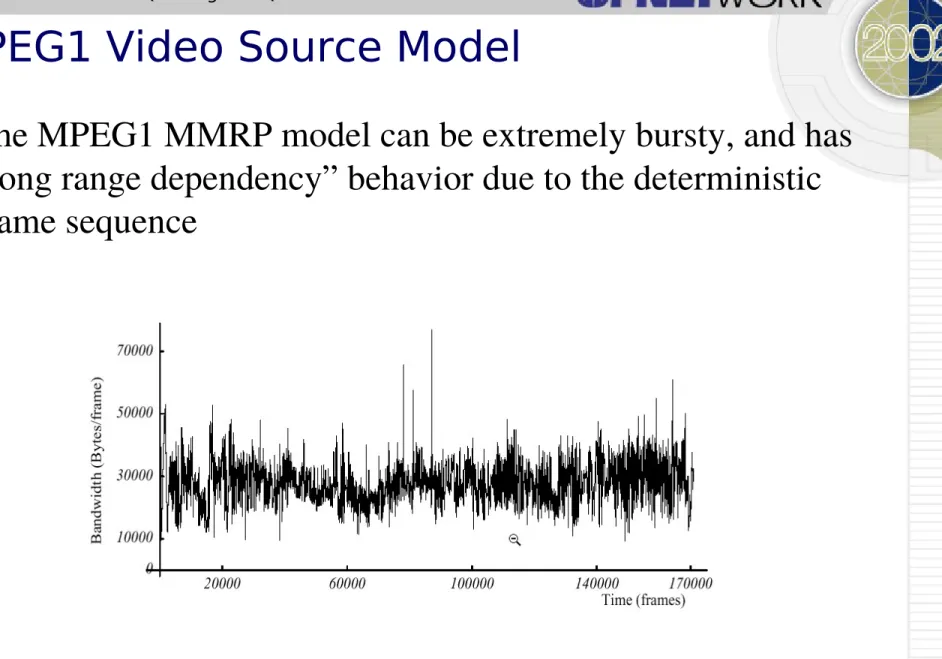
MPEG1 Video Source Model

Diagram Source: Mark W. Garrett and Walter Willinger, “Analysis, Modeling, and Generation of Self-Similar VBR Video Traffic, BELLCORE, 1994

Outline

• Basic concepts • Source models • _{Service models}

– Single vs. multiple-servers

– FIFO, priority, and shared servers

– Demo

• Single-queue systems

• Priority/shared service systems • Networks of queues

Device Queuing Mechanisms

• Common queue examples for IP routers

– FIFO: First In First Out

– PQ: Priority Queuing

– WFQ: Weighted Fair Queuing

– Combinations of the above

• Service types from a queuing theory standpoint

– Single server (one queue - one transmission line)

– Multiple server (one queue - several transmission lines)

– Priority server (several queues with hard priorities - one transmission line)

Single Server FIFO

• Single transmission line serving packets on a FIFO (First-In-First-Out) basis

• Each packet must wait for all packets found in the system to complete transmission, before starting transmission

– Departure Time = Arrival Time + Workload Found in the System +

Transmission time

• Packets arriving to a full buffer are dropped

Arrivals

FIFO Queue

• Packets are placed on outbound link to egress device in FIFO order

Multiple Servers

• Multiple packets are transmitted simultaneously on multiple lines/servers

• Head of the line service: packets wait in a FIFO queue, and when a server becomes free, the first packet goes into service

Arrivals

Priority Servers

• Packets form priority classes (each may have several flows) • There is a separate FIFO queue for each priority class

• Packets of lower priority start transmission only if no higher priority packet is waiting

• Priority types:

– Non-preemptive (high priority packet must wait for a lower priority packet found under transmission upon arrival)

– Preemptive (high priority packet does not have to wait …)

Class 1 Arrivals High Priority

Transmission Line

Class 3 Arrivals Low Priority

Priority Queuing

• Packets are classified into separate queues

– _{E.g., based on source/destination IP address, source/destination TCP port, etc.}

• All packets in a higher priority queue are served before a lower priority queue is served

Shared Servers

• Again we have multiple classes/queues, but they are served with a “soft” priority scheme

• Round-robin

• Weighted fair queuing

Class 1 Arrivals Weight 10

Transmission Line

Class 3 Arrivals Weight 1 Class 2 Arrivals

Round-Robin/Cyclic Service

• Round-robin serves each queue in sequence

– A queue that is empty is skipped

– Each queue when served may have limited service (at most k packets

transmitted with k = 1 or k > 1)

• Round-robin is fair for all queues (as long as some queues do not have longer packets than others)

Fair Queuing

• This scheduling method is inspired by the “most fair” of methods:

– Transmit one bit from each queue in cyclic order (bit-by-bit round robin) – Skip queues that are empty

• To approximate the bit-by-bit processing behavior, for each packet

– _{We calculate upon arrival its “finish time under bit-by-bit round robin”} assuming all other queues are continuously busy, and we transmit by FIFO within each queue

– Transmit next the packet with the minimum finish time

• Important properties:

– Priority is given to short packets

– Equal bandwidth is allocated to all queues that are continuously busy

Finish Time of Packet i i-1 Arrival times

Departure times i

i i-1

Finish Time of Packet i i-1 Arrival times

Departure times i

Weighted Fair Queuing

• Fair queuing cannot be used to implement bandwidth allocation and soft priorities

• Weighted fair queuing is a variation that corrects this deficiency

– _{Let wk be the weight of the k}th queue

– _{Think of round-robin with queue k transmitting wk bits upon its turn}

– If all queues have always something to send, the kth queue receives bandwidth

equal to a fraction w_k / _i w_i of the total bandwidth

• Fair queuing corresponds to w_k = 1

• Priority queuing corresponds to the weights being very high as we move to higher priorities

• Again, to deal with the segmentation problem, we approximate as follows: For each packet:

– We calculate its “finish time” (under the weighted bit-by-bit round robin scheme)

Weighted Fair Queuing Illustration

Combination of Several Queuing

Schemes

Demo: FIFO

FIFO

Demo: FIFO Queuing Delay

Applications have different requirements

• Video

» delay, jitter

• FTP

» packet loss

Control beyond “best effort” needed

• Priority Queuing (PQ)

Demo: Priority Queuing (PQ)

PQ

Demo: PQ Queuing Delays

FIFO

PQ Video

Demo: Weighted Fair Queuing (WFQ)

WFQ

Demo: WFQ Queuing Delays

FIFO

WFQ/PQ Video

PQ FTP

Queuing: Take Away Points

• Choice of queuing mechanism can have a profound effect on performance

• To achieve desired service differentiation, appropriate queuing mechanisms can be used

• Complex queuing mechanisms may require simulation techniques to analyze behavior

Outline

• Basic concepts • Source models

• Service models (demo) • _{Single-queue systems}

– M/M/1……M/M/m/k – _{M/G/1……G/G/1}

– Demo: Analytics vs. simulation

• Priority/shared service systems • Networks of queues

M/M/1 System

• Nomenclature: M stands for “Memoryless” (a property of the exponential distribution)

– _{M/M/1 stands for Poisson arrival process (which is memoryless)}

– M/M/1 stands for exponentially distributed transmission times

• Assumptions:

– Arrival process is Poisson with rate packets/sec

– Packet transmission times are exponentially distributed with mean 1/_

– One server

– Independent interarrival times and packet transmission times

• Transmission time is proportional to packet length • Note 1/ is secs/packet so  is packets/sec (packet

transmission rate of the queue)

Delay Calculation

• Let

Q = Average time spent waiting in queue

T = Average packet delay (transmission plus queuing) • Note that T = 1/ + Q

• Also by Little’s law

N = T and Nq = Q

where

Nq = Average number waiting in queue

• The analysis gives the steady-state probabilities of

number of packets in queue or transmission

• P{n packets} =



(1-



) where



=



/



• From this we can get the averages:

N = _{/(1 -} ₎

T = N/ ₌ _/_{(1 -} _{) = 1/(} _- ₎



N

1

0 _

T



0



Example: How Delay Scales with

Bandwidth

• Occupancy and delay formulas

N = _{/(1 -} _{) T = 1/(} _- ₎ ₌ _/ • Assume:

– _{Traffic arrival rate}  _{is doubled}

– _{System transmission capacity}  _{is doubled}

• Then:

– Queue sizes stay at the same level (_ stays the same) – Packet delay is cut in half ( and are doubled

• A conclusion: In high speed networks

M/M/m, M/M/



System

• Same as M/M/1, but it has m (or



) servers

• In M/M/m, the packet at the head of the queue moves

to service when a server becomes free

• Qualitative result

– Delay increases to _as₌ _/m_{approaches 1}

Finite Buffer Systems: M/M/m/k

• The M/M/m/k system

– Same as M/M/m, but there is buffer space for at most k packets. Packets arriving at a full buffer are dropped

• Formulas for average delay, steady-state occupancy

probabilities, and loss probability

Characteristics of M/M/. Systems

• Advantage: Simple analytical formulas

• Disadvantages:

– The Poisson assumption may be violated

– The exponential transmission time distribution is an approximation at best

– Interarrival and packet transmission times may be dependent (particularly in the network core)

M/G/1 System

• Same as M/M/1 but the packet transmission time

distribution is general, with given mean 1/



and

variance



• Utilization factor



=



/



• Pollaczek-Kinchine formula for

Average time in queue = ₍2 + 1/2)/2(1- )

Average delay = 1/ ₊ ₍2 + 1/2)/2(1- )

• The formulas for the steady-state occupancy

probabilities are more complicated

G/G/1 System

• Same as M/G/1 but now the packet interarrival time

distribution is also general, with mean



and

variance



• We still assume FIFO and independent interarrival

times and packet transmission times

• Heavy traffic approximation:

Average time in queue ~ (2 + 2)/2(1- )

Demo: M/G/1

Packet inter-arrival times

exponential (0.02) sec

Capacity

1 Mbps

Packet size

1250 bytes (10000 bits)

Packet size distribution: exponential

Demo: M/G/1 Analytical Results

Packet Size

Distribution Delay T (sec) Queue Size (packets)

Exponential

mean = 10000 variance = 1.0 *108

0.02 1.0

Constant

mean = 10000

variance = N/A

0.015 0.75

Lognormal

mean = 10000

variance = 9.0 *108

Demo: M/G/1 Simulation Results

Demo: M/G/1 Limitations

Application traffic mix not memoryless

• Video

» constant packet inter-arrivals

• _Http

» bursty traffic

Delay

P-K formula

Outline

• Basic concepts • Source models

• Service models (demo) • Single-queue systems

• _{Priority/shared service systems}

– Preemptive vs. non-preemptive – Cyclic, WFQ, PQ systems

– Demo: Simulation results

• Networks of queues

Non-preemptive Priority Systems

• We distinguish between different classes of traffic (flows) • Non-preemptive priority: packet under transmission is not

preempted by a packet of higher priority • P-K formula for delay generalizes

Class 1 Arrivals High Priority

Transmission Line

Class 3 Arrivals Low Priority

Cyclic Service Systems

• Multiple flows, each with its own queue

• Fair system: Each flow gets access to the transmission line in turn

• Several possible assumptions about how many packets each flow can transmit when it gets access

• Formulas for delay under M/G/1 type assumptions are available

Class 1

Arrivals Transmission Line

Weighted Fair Queuing

Outline

• Basic concepts • Source models

• Service models (demo) • Single-queue systems

• Priority/shared service systems • Networks of queues

– Violation of M/M/. assumptions

– Effects on delays and traffic shaping – Analytical approximations

Two Queues in Series

• First queue shapes the traffic into second queue • Arrival times and packet lengths are correlated

• M/M/1 and M/G/1 formulas yield significant error for second queue

Time

First Queue

Time

Two bottlenecks in series

Bottleneck

Exponential inter-arrivals

Bottleneck

Approximations

• Kleinrock independence approximation

– Perform a delay calculation in each queue independently of other queues

– Add the results (including propagation delay)

• Note: In the preceding example, the Kleinrock independence approximation overestimates the queuing delay by 100%

• Tends to be more accurate in networks with “lots of traffic

Outline

• Basic concepts • Source models

• Service models (demo) • Single-queue systems

• Priority/shared service systems • Networks of queues

• _{Hybrid simulation}

– Explicit vs. aggregated traffic – Conceptual Framework

Basic Concepts of Hybrid Simulation

• Aims to combine the best of analytical results and simulation • Achieve significant gain in simulation speed with little loss of

accuracy

• Divides the traffic through a node into _explicit and

background

– Explicit traffic is simulated accurately – Background traffic is aggregated

• The interaction of explicit and background is modeled either analytically or through a “fast” simulation (or a combination)

Explicit

Explicit Traffic

• Modeled in detail, including the effects of various protocols

• Each packet’s arrival and departure times are recorded (together with other data of interest, e.g., loss, etc.) along each link that it traverses

• Departure times at a link are the arrival times at the next link (plus propagation delay)

• Objective: At each link, given the arrival times (and the packet lengths), determine the departure times

Time

a1 a2 a3 a4

d1 d2 d3 d4

. . .

. . .

Delay Delay Delay Delay

Arrival times at a link

Aggregated Traffic

• Simplified modeling

– We don’t keep track of individual packets, only workload counts (number of packets or bytes)

– We “generate” workload counts

» by probabilistic/analytical modeling, or » by simplified simulation

• Aggregated (or background) traffic is local (per link) • Shaping effects are complex to incorporate

Hybrid Simulation (FIFO Links):

Conceptual Framework

• Given the arrival time ak of the kth explicit packet

• Generate the workload wk found in queue by the kth packet

• From a_k and w_k generate the departure time of the kth packet as

Departure Time d_k = a_k + w_k + s_k

where s_k is the transmission time of the kth packet

Time

aK wK aK+1 wK+1

dK = aK + wK + sK

Explicit Explicit

Explicit Explicit

Background Background

ARRIVAL TIMES

Simulating the Background Traffic Effects

• Use a traffic descriptor for the background traffic (e.g., carried by special packets)

• Traffic descriptor includes:

– Traffic volume information (e.g., packets/sec, bits/sec) – Probability distribution of interarrival times

– Probability distribution of packet lengths – Time interval of validity of the descriptor

• Generate w_k using one of several ideas and combinations thereof

– Successive sampling (for FIFO case)

– Steady-state queue length distribution (if we can get it)

Hybrid Simulation (FIFO Case)

• Critical Question: Given arrival times ak and ak+1, workload wk, and background traffic descriptor, how do we find w_k+1?

• Note: wk+1 consists of wk and two more terms: – Background arrivals in interval a_k+1 - a_k

– (Minus) transmitted workload in interval a_k+1 - a_k • Must calculate/simulate the two terms

• The first term is simulated based on the traffic descriptor of the background traffic • The second term is easily calculated if the queue is continuously busy in ak+1 - ak

Time

a₁ a_{2 a3}

. . .

. . .

Arrival times/Workload found

w₁ w_{2 w3}

d₁ = a₁ + w₁ + s₁ d2 = a2 + w2 + s2 d3 = a3 + w3 + s3

Short Interval Case (Easy Case)

• Short interval ak+1 - ak (i.e., ak+1 < dk)

• Queue is busy continuously in ak+1 - ak

• So wk+1 is quickly simulated

– Sample the background traffic arrival distribution to simulate the new workload arrivals in a_k+1 - a_k

– Do the accounting (add to w_k and subtract the transmitted workload in a_k+1 - a_k )

k d a_k Time

. . .

w_k+1 = w_k + (New bkg arrivals) - (Old bkg transmissions)

d a_k+1 w_k+1

Long Interval Case

• Long interval a_k+1 - a_k (i.e., a_k+1 > d_k)

• Queue may be idle during portions of the interval a_k+1 - a_k • Need to generate/simulate

– _{The new arrivals in ak+1 - ak}

– The lengths of the busy periods and the idle periods

• Can be done by sampling the background arrival distribution in each busy period

• Other alternatives are possible

Time

. . .

Long Interval

ak w_k ak+1 wk+1

dk

Idle Periods

Busy Periods

Steady-State Queue Length Distribution

• If the interval between two successive explicit packets is very long, we can assume that the queue found by the second

packet is in steady state

• So, we can obtain w_k+1 by sampling the steady-state distribution

• Applies to cases where the steady-state distribution can be found or can be reasonably approximated

– M/M/1 and other M/M/. Queues

Micro Simulation: Conceptual Framework

• Handles complex queuing systems

– Micro-packets are generated to represent traffic load within the context of the queue only (i.e., they are not transmitted to any external links) – For long intervals, where convergence to a steady-state is likely

» Try to detect convergence during the microsim » Estimate steady-state queue length distribution

» Sample the steady state distribution to estimate wk+1

• Microsim speeds up the simulation without sacrificing accuracy

• Microsim provides a general framework

– Applies to non-stationary background traffic

Examples of Applications

Analytical Modeling Discrete-Event Simulation

M/G/./. & G/G/./. FIFO Analysis M/G/./. & G/G/./. Priority Analysis Decomposition with Kleinrock Independence Assumption

DES only with Explicit Traffic Hybrid DES with Explicit and Background Traffic

Single Link with FIFO Service

Best Effort Service for Standard Data Traffic Yes N/A N/A Yes Yes

Best Effort Service for LRD/Self-Similar

Behavior Traffic Yes N/A N/A Yes Yes

"Chancing It" with Best Effort Service for

Voice, Video and Data Yes N/A N/A Yes Yes

Single Link with QoS-Based Queueing Using QoS to differentiate service levels for

the same type of traffic N/A

Yes (loss of

accuracy) N/A Yes Yes

Using QoS to support different requirements for different application types given as a detailed study of setting Cisco Router queueing parameters

N/A Highly

approximate N/A Yes Yes

Network of Queues

General network model extending the

previous QoS queueing model N/A

Hop-by-hop Analysis (loss

of accuacy)

Yes (some loss of accuracy - e.g., traffic

shaping)

Yes (Run time a function of network

complexity)

Yes [Fast with minimal loss of

accuracy]

Reduction of the general model to a

representative end-to-end path N/A

Hop-by-hop Analysis (loss

of accuacy)

N/A

Yes (Run time a function of network

complexity)

Yes [Fast with minimal loss of

accuracy]

Demo End-to-end Delay: Baseline Network

Traffic modeled as

1) Explicit traffic

Target Flow: ETE delay as a function of ToS

Target flow: Seattle  Houston - modeled using explicit traffic

– Varying its Type of Service (ToS)

» Best Effort (0)

Explicit Simulation Results for Target Flow

– Total traffic volume » 500 Mbps

– Time modeled

» 35 minutes

– _{Simulation duration}

Hybrid Simulation Results for Target Flow

– Total traffic volume » 500 Mbps

– Time modeled

» 35 minutes

– _{Simulation duration}

References

• Networking

– Bertsekas and Gallager, Data Networks, Prentice-Hall, 1992

• Device Queuing Implementations

– Vegesna, IP Quality of Service, Ciscopress.com, 2001 – _{http://www.juniper.net/techcenter/techpapers/200020.pdf}

• Probability and Queuing Models

– Bertsekas and Tsitsiklis, Introduction to Probability, Athena Scientific, 2002,

http://www.athenasc.com/probbook.html

– Cohen, The Single Server Queue, North-Holland, 1992

– Takagi, Queuing Analysis: A Foundation of Performance Evaluation. (3 Volumes), North-Holland, 1991

– Gross and Harris, Fundamentals of Queuing Theory, Wiley, 1985 – Cooper, Introduction to Queuing Theory, CEEPress, 1981

• OPNET Hybrid Simulation and Micro Simulation

– See Case Studies papers in