Two-phase modelling of debris flow over composite topography: theoretical and numerical aspects

Doctoral School in Environmental Engineering

Two-phase modelling

of debris flow over

composite topography:

theoretical and numerical

aspects

Daniel Zugliani

Department of Civil, Environmental and Mechanical Engineering, University of Trento

Academic year 2013/2014

Supervisor: Prof. Giorgio Rosatti, DICAM, University of Trento

University of Trento Trento, Italy

Acknowledgments

First and foremost, I offer my gratitude to my supervisor, Prof. Giorgio Rosatti, who has supported me with his knowledge and patience. In addition, I thank Nadia Zorzi for her help in the writing process and Giulia Graregnani for her support during the enrollment and the first year of my PhD.

Contents

Acknowledgments iii

Contents viii

List of Figures xiv

List of Tables xv

Summary xvii

I

Derivation and eigenstructure analysis of the

two-phase flow equations over fixed and mobile bed

1

1 Continuum formulations for liquid-granular mixture flows 3 1.1 Ensemble average for continuous fluid phase and discrete

par-ticles . . . 4

1.1.1 Definitions . . . 5

1.1.2 Fluid phase equations . . . 9

1.1.3 Solid phase equations . . . 10

1.1.4 Final set of ensembe averaged equations for conitnuum liquid-granular mixture flow . . . 11

1.2 Volume average for continuous fluid phase and discrete particles 12 1.2.1 Definitions . . . 12

1.2.2 Fluid phase equations . . . 16

1.2.4 Final set of volume averaged equations for continuum

liquid-granular mixture flow . . . 17

1.3 Average approaches for continuous fluid and solid phase . . . . 18

1.4 Comparison of the 3D continuum liquid-granular systems . . . 21

1.5 Closure relations . . . 24

2 The shallow flow approximation 27 2.1 Debris flow characteristic scales . . . 28

2.2 Simplification of the momentum equations on the normal di-rection . . . 33

2.3 Simplification of the momentum equations on the planar di-rection . . . 36

2.4 Number of closure relations needed . . . 38

3 Two-dimensional modelling 41 3.1 Fully two-phase free-surface mobile bed system . . . 42

3.1.1 Boundary conditions . . . 43

3.1.2 Continuity equations . . . 47

3.1.3 Momentum equations . . . 50

3.1.4 Final set of mobile bed motion equations and closure relations . . . 60

3.2 Fully two-phase free-surface fixed bed system . . . 62

3.2.1 Continuity equations . . . 62

3.2.2 Momentum equations . . . 63

3.2.3 Final set of fixed bed motion equations and closure relations . . . 64

3.3 Isokinetic models . . . 65

3.3.1 Mobile bed isokinetic model . . . 66

3.3.2 Fixed bed isokinetic model . . . 69

3.4 Brief literature review . . . 69

4 One-dimensional isokinetic modelling 73 4.1 One-dimensional systems with low sediment concentration . . 76

4.2 One-dimensional systems for high sediment concentration . . . 78

Contents vii

5 Eigenstructure of the one-dimensional models 83 5.1 One-dimensional systems with low sediment concentration . . 85 5.2 One-dimensional systems for high sediment concentration . . . 89 5.3 Two-dimensional plane-wave systems . . . 94

II

Transition from fixed bed to mobile bed:

mathe-matical aspect

99

6 Fixed and mobile-bed flows: possible coupled phenomena 101 6.1 Literature review . . . 103 6.2 A novel approach for the coupling of fixed and mobile bed

systems . . . 104 7 The Composite Riemann Problem: definition, solution and

eigenstructure 107

7.1 The Composite Riemann problem . . . 108 7.1.1 Expected features of the CRP solutions and the

Gen-eralized Rankine-Hugoniot relation . . . 110 7.2 The CRP solution strategy: the Composite PDEs system . . . 111 7.3 Eigenstructure and shock relations of the CPDEs . . . 116 7.4 Classes of solutions of the CRP . . . 122 8 Application of the CRP procedure to high sediment cases 127 8.1 CPDEs system for one-dimensional case . . . 128 8.1.1 Eigenstructure and shock relation of the CPDEs . . . . 130 8.2 CPDEs for two-dimensional plane wave case . . . 134 8.2.1 Eigenstructure and shock relation for the CPDEs . . . 137

III

Transition from fixed bed to mobile bed:

nu-merical aspect

143

9.2.1 A novel Extended Multiple Averages procedure . . . . 153

9.2.2 Application of the EMAs . . . 154

9.3 The Universal Osher solver . . . 158

9.3.1 The Universal Osher solver for partially non-conservative system . . . 161

9.3.2 A new Universal Osher solver with Primitive reconsti-tution . . . 162

9.4 Comparison between the three numerical Riemann solver . . . 166

10 Numerical applications of the CRP 171 10.1 Riemann problems . . . 172

10.1.1 CPDEs model for low sediment concentration . . . 172

10.1.2 CPDEs model for high sediment concentration . . . 181

10.1.3 CPDEs plane-wave model . . . 187

10.2 Realistic application . . . 193

10.2.1 Trench evolution . . . 193

Conclusions

197

List of Figures

1.1 Sketch of the configuration CN with the reference system. . . 5 1.2 Sketch of the variable involved in the volume average with the

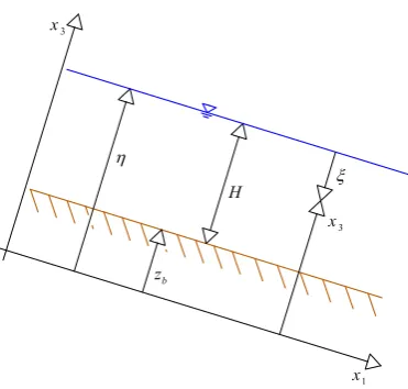
reference system. . . 13 2.1 Sketch of the reference system and the angle of inclination α

respect the gravity force. . . 28 3.1 Sketch of the main variables of the problem. . . 44 3.2 Sketch of a generic stress vector R applied on a surface with

normal ˆn. . . 45 3.3 Sketch of a qualitative profile of the concentration c and

ve-locity u along x3 for an hyperconcentrated flow over mobile

bed. . . 50 3.4 Sketch of the reference system with the direction ξ. . . 51 4.1 Sketch with the indication of the variables for: (a) fixed-bed

case, (b) mobile-bed case. . . 77 5.1 Possible wave patterns of a fixed-bed RP as a function of

the Froude number of the flow near the origin - (A) subcrit-ical flow, (B) supercritsubcrit-ical flow. Velocity is assumed positive throughout. . . 87 5.2 Wave patterns of a mobile-bed RP. Velocity is assumed

5.3 Dimensionless eigenvalues for fixed bed (green), low concen-tration mobile bed (blue) and high concenconcen-tration mobile bed (red): (a) low transport capacity case, (b) high transport ca-pacity case. The parameters used are: ∆ = 1.65 andcb = 0.65. Black dots represent the concentration. . . 93

6.1 Example of transition between mobile bed and fixed bed in Cismon creek. . . 102 6.2 Example of a fixed-bed transect computation using the

method-ology developed by Rulot et al.. . . 104 6.3 Sketch of a CRP describing the transition between mobile and

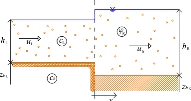
fixed bed with the main variables involved. . . 105

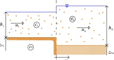
7.1 Sketch of the initial values of a Composite Riemann Problem with a mobile-bed condition on the left of the discontinuity and with a fixed-bed one on the right. . . 109 7.2 The four different classes of CRP solutions for positive

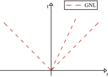
ve-locity in the neighborhood of the origin: (a) FBsub-MB, (b) FBsup-MB, (c) MB-FBsub, (d)MB-FBsup. Dashed lines rep-resent mobile-bed fields, solid lines fixed-bed ones. GNL repre-sent genuinely nonlinear fields, LD classical linearly degenerate fields and LD∗ linearly degenerate fields with λ independent from U. . . 124 7.3 Example of two possible exact solutions of a RP of MB-FBsup

type. All the waves are entropy satisfying. . . 126

List of Figures xi

9.1 Comparison between analytical (solid line) and numerical solu-tions obtained with LHLL without (blue dots) and with (red circles) F2 correction for the transition between mobile and

fixed bed case. On the left subfigure: free surface η and bed elevation zb; on the right: detail of the bottom elevation near the interface. . . 148 9.2 Comparison between analytical (solid line) and numerical

so-lutions obtained with LHLL (blue dots), CIGR (red dots) and UOP (green dots) numerical solvers for the transition between fixed and mobile bed case. On the left subfigure: free surface

η and bed elevation zb; on the right: details of the bottom elevation near the interface. . . 168 9.3 Comparison between analytical (solid line) and numerical

so-lutions obtained with LHLL (blue dots), CIGR (red dots) and UOP (green dots) numerical solvers for the transition between mobile and fixed bed case. On the left subfigure: free surface

η and bed elevation zb; on the right: detail of the bottom elevation near the interface. . . 169

10.1 Comparison between analytical (solid line) and numerical (cir-cles) solutions of the free surfaceηand the bed levelzb for the pure fixed-bed (on the left) and the pure mobile-bed (on the right) RP test case. . . 173 10.2 Comparison between analytical (solid line) and numerical

(cir-cles) solutions of the FBsub-MB test case. Clockwise from upper left subfigure: free surface η and bed level zb, velocity

u, Froude number u/√gh, equilibrium and transported con-centrations ϕ,c. . . 174 10.3 Details of the behavior of the concentration (on the left) and of

10.4 Comparison between analytical (solid line) and numerical (cir-cles) solutions of the FBsup-MB test case. Clockwise from upper left subfigure: free surface η and bed level zb, velocity

u, Froude number u/√gh, equilibrium and transported con-centrations ϕ, c. . . 176 10.5 Comparison between analytical (solid line) and numerical

(cir-cles) solutions of the MB-FBsub test case. Clockwise from upper left subfigure: free surface η and bed level zb, velocity

u, Froude number u/√gh, equilibrium and transported con-centrations ϕ, c. . . 177 10.6 Comparison between analytical (solid line) and numerical

(cir-cles) solutions of the MB-FBsup test case. Clockwise from upper left subfigure: free surface η and bed level zb, velocity

u, Froude number u/√gh, equilibrium and transported con-centrations ϕ, c. . . 178 10.7 Details of the bottom elevation near the interface between

fixed and mobile bed for the MB-FBsup test case. . . 179 10.8 Comparison of the exact solution (solid line) with the first

order solution (red circles) and the second order one (black dots) for a resonant case relevant to a mobile-fixed transition. 179 10.9 Comparison of the exact solution (solid line) with the first

order solution (circles) and the second order one (dots) for a resonant case relevant to a fixed-mobile transition. . . 180 10.10Comparison between analytical (solid line) and numerical

(cir-cles) solutions of the FBsub-MB test case. Clockwise from upper left subfigure: free surface η and bed level zb, velocity

u, Froude number u/√gh, equilibrium and transported con-centrations ϕ, c. . . 182 10.11Details of the behavior of the concentration (on the left) and of

List of Figures xiii

10.12Comparison between analytical (solid line) and numerical (cir-cles) solutions of the FBsup-MB test case. Clockwise from upper left subfigure: free surface η and bed level zb, velocity

u, Froude number u/√gh, equilibrium and transported con-centrations ϕ,c. . . 184 10.13Comparison between analytical (solid line) and numerical

(cir-cles) solutions of the MB-FBsub test case. Clockwise from upper left subfigure: free surface η and bed level zb, velocity

u, Froude number u/√gh, equilibrium and transported con-centrations ϕ,c. . . 185 10.14Details of the bottom elevation near the interface between

fixed and mobile bed for the MB-FBsub test case. . . 185 10.15Comparison between analytical (solid line) and numerical

(cir-cles) solutions of the MB-FBsup test case. Clockwise from upper left subfigure: free surface η and bed level zb, velocity

u, Froude number u/√gh, equilibrium and transported con-centrations ϕ,c. . . 186 10.16Comparison between analytical (solid line) and numerical

(cir-cles) solutions of the FBsub-MB test case. Clockwise from upper left subfigure: free surface ηand bed level zb, velocities

u (red) andv (blue), Froude number u/√gh, equilibrium and transported concentrations ϕ, c. . . 188 10.17Details of the behavior of the concentration (on the left) and of

the bottom elevation (on the right) near the interface between fixed and mobile bed for the FBsub-MB test case. . . 189 10.18Comparison between analytical (solid line) and numerical

(cir-cles) solutions of the FBsup-MB test case. Clockwise from upper left subfigure: free surface ηand bed level zb, velocities

10.19Comparison between analytical (solid line) and numerical (cir-cles) solutions of the MB-FBsub test case. Clockwise from upper left subfigure: free surface η and bed level zb, velocities

u (red) andv (blue), Froude number u/√gh, equilibrium and transported concentrations ϕ,c. . . 191 10.20Details of the bottom elevation near the interface between

fixed and mobile bed for the MB-FBsub test case. . . 191 10.21Comparison between analytical (solid line) and numerical

(cir-cles) solutions of the MB-FBsup test case. Clockwise from upper left subfigure: free surface η and bed level zb, velocities

u (red) andv (blue), Froude number u/√gh, equilibrium and transported concentrations ϕ,c. . . 192 10.22Initial condition of the trench. On the left the free surface and

the bottom elevation, on the right the concentration. . . 194 10.23Evolution of a trench: approaching the fixed bed transect. On

the left the free surface and the bottom elevation, on the right the concentration. . . 195 10.24Evolution of a trench: inside the fixed bed transect. On the

left the free surface and the bottom elevation, on the right the concentration. . . 195 10.25Evolution of a trench: approaching the downstream mobile

bed transect. On the left the free surface and the bottom elevation, on the right the concentration. . . 196 10.26Evolution of a trench: trench moving in the downstream

List of Tables

7.1 Summary of the possible characteristic fields with indication of the variables that remain constant across each wave of that field. Meanings of the symbols: GNL = genuinely nonlinear field; LD = classical linearly degenerate field; LD∗ = linearly degenerate field with λ independent from U. Finally ξ is a degree of freedom of the fifth field . . . 120 8.1 Summary of the possible characteristic fields with indication

of the variables that remain constant across each wave of that field. Meanings of the symbols: GNL = genuinely nonlinear field; LD = classical linearly degenerate field; LD∗ = linearly degenerate field with λ independent from U. Finally ξ is a degree of freedom of the fifth field . . . 140 9.1 Initial values used for the fixed to mobile bed transition, and

mobile to fixed bed transition RPs test case. . . 167 10.1 Initial values used for the pure fixed-bed and the pure

Summary

In the mountain territory the majority of the population and of the produc-tive activities are concentrated in the proximity of torrents or over alluvial fans. Here, when intense rainfall occurs, debris flow or hyper-concentrated flow events can produce serious problems to the population with possible casualties. On the other hand, the majority of these problems could be overcome with accurate hazard mapping, disaster prevention planning and mitigation structures (e.g. silt check dams, paved channels, weirs ...). Good and reliable mathematical and numerical models, able to accurately describe these phenomena are therefore necessary.

In the framework of finite-volume methods with Godunov approach, the fluxes are evaluated solving a Riemann Problem (RP). A RP is an initial value problem related to a set of PDEs equations wherein, in a certain point, there is a discontinuity separating different left and right initial constant states. However, if the topography is composite, a new type of Riemann problem, called Composite Riemann Problem (CRP), occurs. In a CRP, not only the initial constant states, but also the relevant PDEs systems change across the discontinuity. This additional complexity makes the general solu-tion of the CRP quite challenging to obtain.

The first part of the work is devoted to the derivation of the PDEs systems describing the fixed- and mobile-bed behaviors. Starting from the 3D discrete equations valid for each phase (continuous fluid and solid granular) and us-ing suitable average processes the 3D continuous equations (continuous fluid and solid) are obtained. Introducing the shallow water approximation and performing the depth average process, the 2D fully two-phase models for free-surface flow over fixed- and mobile-bed are derived. The isokinetic ap-proximation, which states the equality between the velocity of the solid phase and the liquid phase, is then used, ending up with the so-called two-phase isokinetic models. Finally, an exhaustive comparison between the fixed- and the mobile-bed fully two-phase models, the two-phase isokinetic models and others models proposed in the literature is presented.

xix

From the numerical point of view, all the developed Composite systems are integrated using the finite-volume method with Godunov fluxes. These fluxes are evaluated using three different approximated Riemann solvers: the Gen-eralized Roe solver, the LHLL solver and the Universal Osher solver. All the solvers are analyzed and an exhaustive comparison between them is per-formed, highlighting pros and cons. The schemes are second order accurate in space and time, and this has been achieved by means of the MUSCL ap-proach. Finally numerical schemes have been parallelized using OpenMP standard.

Part I

Derivation and eigenstructure

analysis of the two-phase flow

equations over fixed and mobile

Chapter 1

Continuum formulations for

liquid-granular mixture flows

From a physical point of view, a liquid-granular flow is a gravity-driven move-ment of a mixture composed by a granular phase, usually sand or gravel, and by a fluid phase surrounding the solid one. The problem can be faced with the use of an appropriate set of three-dimensional partial differential equa-tions that describe the interstitial fluid and an equation of motion for the center of mass each single particle. The variables related to a specific phase of the mixture are therefore defined only in the space actually occupied by the phase itself. However, this approach has a practical problem: when we approach real scale phenomena, the number of equations needed to describe all the particles in a debris flow or hyperconcentrated flow becomes larger and larger producing an unmanageable system. A possible solution is switching to a continuum description of the liquid-granular mixture. With this type of formulation, unlike before, a generic variable related to one phase (both fluid and solid) is defined in every point of the mixture flow domain, even where a phase does not actually occupy the space. The definition of such variables is possible only by means of appropriated average.

This approach was used in the works of Zhang and Prosperetti [67, 68] where the authors use a statistical ensemble average, and the works of Anderson and Jackson [5] and Jackson [35, 36] where a volume average is used.

descrip-tion of both the fluid and the solid constituent. Although, as said before, a mixture is the sum of fluid and solid components, the continuum descrip-tion of this mixture is not obtained simply adding together the equadescrip-tions for the fluid and solid phases described as continuum, but an indicator function must be introduced in order to recognize which phase occupy a certain point of the space. The introduction of the indicator function leads to a discrete definition of the variables, so an appropriate average process (e.g. ensemble or volume) has to be used in order to obtain a continuum formulations for the liquid-granular mixture. Among this class of derivation we cite the works of Drew [21], Hill [32] and Joseph and Lundgren [38].

In this Chapter we analyze the approaches presented in the literature in order to have a clear understand of the terms involved in the three dimen-sional differential equations that describe the liquid-granular mixture flows. Moreover a unified approach has been presented, since, different approaches produce slightly different partial differential equations. In particular, we fo-cus our attention on first approach in Section 1.1 where the ensemble average is presented, and in Section 1.2 where the volume average is described. The second approach is briefly introduced in Section 1.3, while in Section 1.4 a comparison between the different approaches is presented with the defini-tion of an unified model. Finally, in Secdefini-tion 1.5 some aspects related to the closure of the problem are introduced.

1.1

Ensemble average for continuous fluid phase

and discrete particles

Given a set of measurements regarding a debris flow or an hyperconcentrated flow with certain macroscopic conditions (e.g. flow depth, fluid and solid discharge), the microscopic characteristics, measured during each realization, are different from one to each other. As for the turbulence, the study of the pointwise properties for this type of flow is based on the use of the ensemble average.

1.1 Ensemble average for continuous fluid phase and discrete particles 5

use, as starting point, the equation of motion of a set of spherical particles of radius r surrounded by an inviscid [67] or a viscous fluid [68]. In the follow only the main aspect of the derivation are presented, while we refer to the original article for the complete derivation.

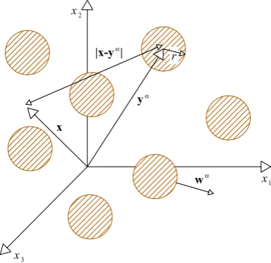
1.1.1

Definitions

A configuration CN of a mixture flow is defined by a number N of spherical particles of radius r, with instantaneous position yα and velocity wα (with

α = 1. . . N), and a fluid which surrounds the particles (see Figure 1.1 for an overview of a configuration CN). It is possible to define the indicator

Figure 1.1: Sketch of the configuration CN _{with the reference system.} function for the fluid phase associated to the configuration CN as

χF(x;CN) =

(

1 if x is in the fluid phase

0 otherwise (1.1)

while the indicator function for the solid phase, due to impenetrability of the two phases, is

χS(x;CN) = 1−χF(x;CN) (1.2)

Introducing the Heaviside step function defined as

H(x) =

(

0 if x <0

the indicator function for the solid phase can be written as

χS(x;CN) = N

X

α=1

H(r− |x−yα|) (1.4)

where (r− |x−yα_{|) is positive only when the point x is inside the particle}

α located atyα_.

Using this indicator function it is possible to define the volume fractions (also know as volumetric concentration) for the solid phase as

c(x, t) = 1

N!

Z

χS(x;CN)P(CN;t) dCN (1.5) where P(CN_{;t) is the probability density function associated to the} configu-ration CN _{and normalized as}

Z

P CN;t dCN =N!

where the integral is performed all over the configurations. It is also possible to define the reduced one-particle density function as

P (y,w;t) =P (1;t) = 1 (N −1)!

Z

P CN;t dCN−1 (1.6) where the integral is performed all over the possible degrees of freedom of the system except for the ones associated to particle 1.

With this definition and remembering the definition of the solid indicator function, the solid concentration can be defined as

c(x, t) =

Z

|x−y|≤r

Z

P(y,w;t)d3w d3y (1.7)

where now the integral is performed only over the space (d3_{y) and velocity}

(d3_{w) associated to the particles. For the fluid phase, instead, the volume}

concentration is defined as

β(x, t) = 1

N!

Z

χF(x;CN)P(CN;t) dCN

Since the sum of the indicator function is one, the two concentration are correlated by

1.1 Ensemble average for continuous fluid phase and discrete particles 7

The ensemble average of a generic local quantity fF(x, t;CN) related to the fluid phase, at position x, time t, given the configuration CN_{, is defined} as

hfFi(x, t) = 1

N! 1

β

Z

fF(x, t;CN)χF(x;CN)P(CN;t) dCN (1.9) This definition has the advantage that is defined inevery point of the mixture domain, but it has the disadvantage that the integral and the derivative is not commutative due to the discontinuity of the indicator function χF(x;CN).

Performing some algebraic manipulations, it is possible to evaluate the ensemble average of the time and spatial derivative offF(x, t) (we refer to the original articles for the full mathematical manipulation needed) obtaining

∂ ∂tfF

= 1

β

∂

∂tβhfFi+

I

s

Z

w·ˆnhfFi₁P(1;t) d3w dSy

(1.10)

∂ ∂xi

fF

= 1

β

∂ ∂xi

βhfFi −

I

s

Z

ˆ

nhfFi₁P(1;t)d3w dSy

(1.11) where nˆ is the normal unit vector oriented outward from the particle, Sy is the surface of the particle and hfFi1 is the ensemble average of the function

fF where the position and velocity of one particle is a priori defined. These two equations will be fundamental when, in the next Sections, we apply the ensemble average process to the motion equations for the fluid phase.

For a quantity associated to the solid particles as a whole (like center of mass velocity, momentum, ...) it is more useful to introduce a different indicator function describing the particle as a point

χS(x;CN) =υ N

X

α=1

δ(x−yα) (1.12)

where υ is the constant volume of one particle and δ is the Dirac delta function defined as

δ(x) = ∂H(x)

∂x =

(

0 if x6= 0

∞ if x= 0 (1.13)

in which one particle is located in the point x, is

hfS(x, t)i= 1

n(x, t)

Z

f_S(1)(t; 1)P(1, t) d3w (1.14) where n is the particle number density

n(x, t) =

Z

P(1;t) d3w (1.15)

=

Z

P(x,w;t) d3w

Expanding equation (1.7) in Taylor series around x(this is possible since the averaged quantity changes slowly at the scale of particle) and using equation (1.15), a more common definition of the solid concentration is obtained

c(x, t) = υn(x, t) +O

r2 L2

' υn(x, t) (1.16)

where L is a characteristic length scale of the flow field variation.

The ensemble average of total time derivative of the property fS(x, t), associated to the center of mass of a particle, can be written, after some mathematical manipulation (see the original papers for the complete deriva-tion), as

d dtfS

= 1

n

∂

∂t(nhfSi) + ∂ ∂xi

(nhfSwii)

(1.17)

We highlight that, for a fS related to a particle as a whole, so the particle is a points, a Lagrangian approach has to be used. However, when the average process is applied, the averaged function hfSi is define all over the space, so an Eulerian approach can be used. Equation (1.17) defines this passage from a Lagrangian approach to an Eulerian one.

1.1 Ensemble average for continuous fluid phase and discrete particles 9

1.1.2

Fluid phase equations

The local equation for the mass conservation of the incompressible fluid phase, valid, as written before, only when the fluid is present, is

∂ ∂xi

uF_i = 0 (1.18)

where uF is the fluid velocity. Applying the average process to the equation the result is

∂ ∂xi

uF_i

= 0 (1.19)

This equation is not useful, inasmuch it is defined over all the mixture domain due to the average process, but it is not expressed in term of average func-tions. However using equations (1.10), (1.11) and the kinematic boundary condition that states the impenetrability of the solid and fluid phase

w·ˆn=uF ·nˆ (1.20)

the resulting expression is

∂

∂t(β) + ∂ ∂xi

βuF_i = 0 (1.21)

where now only the average variables of the flow compare in the equation. The local momentum balance for the incompressible fluid phase, with constant density ρF, is

ρF

∂ ∂t u

F j

+ρF

∂ ∂xi

uF_i uF_j= ∂

∂xi

T_ijF +ρFgj (1.22) where TF is the local fluid stress tensor and g is the gravity force.

In order to obtain the averaged momentum equation, the procedure is similar to the one used for the continuity equations, ending up with

ρF

∂ ∂t β

uF_j

+ρF

∂ ∂xi

β

uF_i uF_j

=β

∂ ∂xi

T_ijF

+ρFβgj (1.23) However, in this equation some terms are not expressed using average vari-ables (e.g. in the second derivative the average is applied to uF

separately to the functions uF

i and uFj ) so same mathematical manipulation is needed. At the end this expression becomes

ρF

∂ ∂t β

uF_j+ρF

∂ ∂xi

βuF_i uF_j =ρF

∂ ∂xi

βRF_ij+ + ∂

∂xi

β

T_ijF

−F_Fzp_−S,j +ρFβgj (1.24)

where RF

ij is the ij component of the stress tensorRF =−

D

uF

−uF2E

composed by the Reynold like terms (the ensemble average of the square of the difference between the ensemble average fluid velocity and the local fluid velocity) and F_Fzp_−S,j is the j-th component of the interphase forces between fluid and particles Fzp_F−S defined as

Fzp_F−S =

I

s

Z

P (y,w;t)TF₁(x, t; 1)·ˆn d3w dSy (1.25)

1.1.3

Solid phase equations

Using fS = 1 in equation (1.17) it is possible to derive the conservation of the particle density number n

∂

∂t(n) + ∂ ∂xi

(nhwii) = 0 (1.26)

and, using the definition of the solid concentration (1.16) the final result is

∂ ∂t(c) +

∂ ∂xi

(chwii) = 0 (1.27)

remembering that the volume υ of a particle does not change in time and space.

The equation of motion of one particle moving, with other particles, in a viscous fluid is

m d

dt (w) = FC+mg+

I

s

1.1 Ensemble average for continuous fluid phase and discrete particles 11

fluid phase on the surface of the particle s. Applying the ensemble average process to this expression and using equation (1.17), the averaged momentum equation for the solid phase is obtained

∂

∂t(nmhwji) + ∂ ∂xi

(nmhwiwji) =hFCi+mg+ + 1

n

Z

P(x,w;t)

I

s

TF₁(z, t; 1)·nˆ dSz d3w (1.29) As for the fluid momentum equation, same mathematical manipulation are needed in order to express all the terms using only average variable, ending up with

ρS

∂

∂t(chwji) +ρS ∂ ∂xi

(chwii hwji) = ρS

∂ ∂xi

cRS_ij+F_Szp_−F,j+

+nhFC,ji+ρScgj (1.30) where hFC,ji is the j-th component of the average collisional force FC, RSij is the ij component of the stress tensor RS _{= −}

(hwi −w)2

composed by the Reynolds like stress produced by the average process, F_Szp_−F,j is the

j-th component of the interphase forces between solid and fluid phases Fzp_S−F defined as

Fzp_S−F =

Z

P (x,w;t)

I

s

TF₁(z, t; 1)·ˆn dSz d3w (1.31) and ρS is the constant solid density

ρS =

m

υ (1.32)

1.1.4

Final set of ensembe averaged equations for

conit-nuum liquid-granular mixture flow

equations (1.21), (1.24), (1.27) and (1.30) that reads



             

             

∂β

∂t +∇ ·(βuf) = 0 ρf

∂

∂t(βuf) +∇ ·(βufuf)

=ρf∇ · βRF

+∇ · βTF+ −Fzp_F−S+βρfg

∂c

∂t +∇ ·(cw) = 0 ρs

∂

∂t(cw) +∇ ·(cww)

=ρS∇ · cRS

+nFC +Fzp_S−F +cρsg

(1.33)

where, for shake of clarity, we neglect the average symbol.

1.2

Volume average for continuous fluid phase

and discrete particles

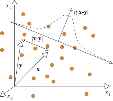
The volume average is performed averaging a quantity over a volume in which there are fluid and particles. This Section is a short review of the works of Anderson and Jackson [5] and Jackson [35, 36]. The authors start from the local differential equations of motion for the fluid phase and the equation of motion for the center of mass of a single particle surrounded by a viscous fluid (as for the ensemble average presented in Section 1.1). Here we present only the basic aspect of the volume average process, while for more exhaustive information about the derivation we refer the reader to the original works.

1.2.1

Definitions

The generic volume average of a function f(x, t) over a sphere of volume V

is define as

hfi(x, t) = 1

V

Z

V

f(y, t) dVy (1.34)

1.2 Volume average for continuous fluid phase and discrete particles 13

However, if in the volume there are two or more phases (see Figure 1.2 for a sketch of the problem), it is possible to introduce a weighting function

g(|x−y|) in order to define the volume average of the generic function as hfi(x, t) =

Z

V(t)

f(y, t)g(|x−y|) dVy (1.35)

where V(t) is the whole volume occupied by the phases that can change in time.

Figure 1.2: Sketch of the variable involved in the volume average with the reference system.

The weighting function is a generic function that has the following prop-erty:

• it is normalized to one

Z

V(t)

g(|x−y|) dVy = 1

• it is positive defined;

An example of this kind of weighting function is a Gaussian function centered in x

For a two phase flow it is possible to divide the total volume V (t) into the fluid one (VF (t)) and the solid one (VS(t)). The average process over these two volumes produce the definition of the fluid and the solid volume fraction

β(x, t) =

Z

VF(t)

g(|x−y|) dVy (1.36)

c(x, t) =

Z

VS(t)

g(|x−y|) dVy (1.37)

and, sinceVF+VF =V, the relation between the two volume fractions follows straightforwardly

β+c= 1

However, since the solid volume is composed of N(t) particles of volume υ, the solid volume fraction can be also written as

c(x, t) = N(t)

X

α=1

Z

υ

g(|x−y|) dVy (1.38)

The particle number density n(x, t) is defined as

n(x, t) = N(t)

X

α=1

g(|x− y_α|) (1.39)

and it is possible to obtain a realtion with the concentration c(x, t) via

n(x, t)' c(x, t)

υ (1.40)

where the order of approximation is Or2 L2

.

The average of a generic function related the fluid phasefF(x, t) is defined as

hfFi(x, t) = 1

β(x, t)

Z

Vf(t)

1.2 Volume average for continuous fluid phase and discrete particles 15

and in a similar way it is possible to define the average of a function regarding the solid phase fS(x, t)

hfSi(x, t) = 1

c(x, t)

Z

VS(t)

fS(y, t)g(|x−y|) dVy (1.42) Nevertheless there are some function fP(xP, t) defined for a particle as a whole (e.g. the center of mass velocity, the angular momentum, ...) for which it is more convenient to use the average based on the particle number

hfPi(x, t) = 1

n(x, t) N(t)

X

α=1

fP(yα, t)g(|x−yα|) (1.43) where yα is the center of the α-th particle.

With some mathematical manipulation (we refer the reader to the original works for the complete derivation), the volume averaged of the time and space derivatives of a function fF(x, t) related to the fluid phase are

∂ ∂tfF

= 1 β   ∂

∂t(βhfFi) +

N(t)

X

α=1

I

sα

fF(y, t)g(|x−y|)wα·ˆnα dSy





(1.44) wherewα andnˆα are the velocity and the normal outward vector of theα-th particle respectively, and the integral is performed all over the surface sα of each particle, and

∂ ∂xi fF = 1 β   ∂ ∂xi

(βhfFi)− N(t)

X

α=1

I

sα

fF(y, t)g(|x−y|) ˆnαi dSy



 (1.45)

where ˆnα

i is thei-th component ofnˆα. The volume average of the total time derivative for a function fP regarding the particles as a whole is instead

d dtfP

= 1 n   ∂

∂t(nhfPi) + ∂ ∂xi

N(t)

X

α=1

fP(yα, t)wαig(|x−yα|)



 (1.46)

1.2.2

Fluid phase equations

Like in the ensemble average, the main objective of this Section (and also the next one) is to derive the averaged equations of motion for the fluid (and solid) phase, constituting the mixture, expressed in term of the average variables that are defined everywhere in the mixture domain.

The averaged mass equation for the incompressible fluid phase is derived, as for the ensemble average, starting from the local equation (1.18). The equation is then averaged over the fluid volume using the definition written in the previous Section. The result is

∂

∂t(β) + ∂ ∂xi

βuF_i = 0 (1.47)

In the same way, starting from the equation (1.22), it is possible to derive the following averaged fluid momentum equation

ρF

∂ ∂t β

uF_j+ρF

∂ ∂xi

βuF_i uF_j =β

∂ ∂xi

T_ijF

+ρFβgj and with some mathematical manipulation this equation becomes

ρF

∂ ∂t β

uF_j+ρF

∂ ∂xi

βuF_i uF_j =ρF

∂ ∂xi

βRF_ij+ + ∂

∂xi

βT_ijF−FF−S,j +ρFβgj (1.48)

where R_ijF is the ij component of the stress tensorRF =−D

uF−uF2

E

composed by the Reynolds like stress produced by the average process and

FF−S,j is thej-th component of the interphase forces between fluid and par-ticles FF−S defined as

FF−S = N

X

α=1

I

sα

TF(y, t)·nˆαg(|x−y|) dSy (1.49)

1.2.3

Solid phase equations

1.2 Volume average for continuous fluid phase and discrete particles 17

average process, it is possible to derive the averaged momentum equation for the solid phase

ρS

∂

∂t(nhwji) +ρS ∂ ∂xi

(nhwjwii) =

n

υ hFC,ji+ρSngj+

+ N

X

α=1

g(|x−yα|)

I

sα

TF ·nˆα dSy

!

j

(1.50)

wherehFC,jiis thej-th component of the averaged collisonal forceFC. With some mathematical manipulation, introducing RS _{= −}

(hwi −w)2 and remembering that c=nυ, the final momentum equation for the solid phase is

ρS

∂

∂t(chwji) +ρS ∂ ∂xi

(chwii hwji) = ρS

∂ ∂xi

cRS_ij+FS−F,j+

+nhFC,ji+ρScgj (1.51) where FS−F,j is the j-th component of the the interphase force exerted by the solid particles on fluid FS−F defined as

FS−F = N

X

α=1

g(|x−yα|)

I

sα

TF (y, t)·ˆnα dSy (1.52)

The conservation of the particle number density is derived from equation (1.46) imposing fP = 1 in equation (1.46) ending up with

∂

∂t(n) + ∂ ∂xi

(nhwii) = 0 (1.53)

Using the definition of n, the conservation of solid mass is then obtained

∂ ∂t(c) +

∂ ∂xi

(chwii) = 0 (1.54)

1.2.4

Final set of volume averaged equations for

con-tinuum liquid-granular mixture flow

equations (1.47), (1.48), (1.54) and (1.51) that reads



             

             

∂β

∂t +∇ ·(βuf) = 0 ρf

∂

∂t(βuf) +∇ ·(βufuf)

=ρf∇ · βRF

+∇ · βTF

+ −FF−S+βρfg

∂c

∂t +∇ ·(cw) = 0 ρs

∂

∂t(cw) +∇ ·(cww)

=ρS∇ · cRS

+nFC+ +FS−F +cρsg

(1.55)

where, for shake of clarity as in the ensemble average, we neglect the average symbol.

1.3

Average approaches for continuous fluid

and solid phase

The second class of approaches present in the literature uses, as said before, a continuous description of both the fluid and the solid constituent as start-ing point. Although a mixture is the sum of fluid and solid components, the continuum description of this mixture is not obtained simply adding together the equations for the fluid and solid phases described as continuum, but an indicator function must be introduced in order to recognize which phase oc-cupy a certain point of the space. The introduction of the indicator function leads to a discrete definition of the variables, so an appropriate average pro-cess (e.g. ensemble or volume) has to be used in order to obtain a continuum formulations for the liquid-granular mixture. Among this class, we briefly summarize here the works of Drew [21], Hill [32] and Joseph and Lundgren [38].

1.3 Average approaches for continuous fluid and solid phase 19

average process. With some mathematical manipulation these equations can be written as



             

             

∂β

∂t +∇ ·(βhufi) = 0 ρf

∂

∂t(βhufi) +∇ ·(βhufi hufi)

=∇ · βRF

+∇ · β

TF

+ + Md_f +pF∇β+βρfg

∂c

∂t +∇ ·(chusi) = 0 ρs

∂

∂t(chusi) +∇ ·(chusi husi)

=∇ · cRS

+∇ · cTS

+ − Md

f +

pF

∇β

+cρsg

(1.56) where the first two equations are the fluid mass and momentum balance, while the last two are the balances of the solid phase. In these equations the solid phase velocity isus, the fluid stress tensor is decomposed in a deviatoric part τ¯F _{and an pressure p}F

TF =τ¯F −pFI (1.57)

where Iis the identity matrix. Similar decomposition is applied to the solid stress tensor, but following the paper, the solid pressure pS _{can be further} decomposed in fluid pressure plus a collisional pressure due to the interaction between the particles

TS =¯τS− pF +pcoI (1.58)

Terms Md f +

pF

∇β includes all the interphase forces (drag, buoyancy, virtual mass effect, ...). In particular we highlight the presence of the gradient of the fluid phase concentration, though this term is not exactly a gradient, but only a way to identify the surfaces of the solid particles. We do not write here the explicit expression ofMd

f due to the complexity of the terms and it is also not relevant for the rest of the discussion.

pressure terms at the interface between the two phases. In this way the final set of equations is

                             ∂β

∂t +∇ ·(βhufi) = 0 ρf

∂

∂t(βhufi) +∇ ·(βhufi hufi)

=∇ · βRF

+∇ · βTF

+ + Mf +

pF

∇β+βρfg

∂c

∂t +∇ ·(chusi) = 0 ρs

∂

∂t(chusi) +∇ ·(chusi husi)

=∇ · cRS

+∇ · cTS

+ − Mf −

pS

∇c+cρsg

(1.59) where the only difference with the one obtained by Drew (1.56) is in the terms related to the interphase forces that now areMf plus the terms

pF∇β for the fluid phase andhpsi ∇cfor the solid one. Mf, in this case, contains all the interphase forces plus the Reynolds like terms derived from the decomposition used. Also in this case we do not show the explicit expression of Mf for the same reason as before.

The last average system that we report here is the one proposed by Joseph and Lundgren [38] obtained by te use of an ensemble average. The equations that they derive are the following

                             ∂β

∂t +∇ ·(βhufi) = 0 ρf

∂

∂t(βhufi) +∇ ·(βhufi hufi)

=∇ · βRF

∗

+∇ · βTF

+ − hδSti+βρfg

∂c

∂t +∇ ·(chusi) = 0 ρs

∂

∂t(chusi) +∇ ·(chusi husi)

=∇ · cRS

∗

+∇ · cTS

+ +hδSti+cρsg

(1.60) where RF

∗ and RS∗ are a the Reynolds like stresses due to the averaging

1.4 Comparison of the 3D continuum liquid-granular systems 21

the solid particles. The Reynold stresses presented in this work are slightly different from the previous ones since they include also the indicator function used during the average process.

1.4

Comparison of the 3D continuum

liquid-granular systems

In order to going on with the derivation of the two dimensional shallow flow equations for the two-phase flow over fixed and mobile bed presented in the next Chapters, it is necessary to define an unified model that represent all the systems presented in the previous Sections since they are slightly differ-ent from each other. For this purpose a comparison between the proposed systems is necessary. For sake of clarity, from now on we neglect the symbols of the average.

First of all we say something about the velocity us of the particle com-pared with the velocityw of the center of mass used in Sections 1.1 and 1.2. Following the works of Zhang and Prosperetti [67, 68] and Jackson [36, 35] the velocity us can be expanded in Taylor series as

us=w+ r

2

L2f(Ω) +O

r4

L4

where f(Ω) is a function concerning the angular velocity of the particles. With the same order of approximationO

r2

L2

used in the previous Sections, the two velocity are equal

us 'w (1.61)

so, without adding errors, a switch between them is possible.

Section 1.1 are                              ∂β

∂t +∇ ·(βuf) = 0 ρf

∂

∂t(βuf) +∇ ·(βufuf)

=ρf∇ · βRF

+∇ · βTF+ −Fzp_F−S+βρfg

∂c

∂t +∇ ·(cus) = 0 ρs

∂

∂t(cus) +∇ ·(cusus)

=ρS∇ · cRS+nFC+ +Fzp_S−F +cρsg

(1.62)

With the same approximation for the solid velocity, the volume averaged equations (1.55) derived in Section 1.2 constitute the following system

                             ∂β

∂t +∇ ·(βuf) = 0 ρf

∂

∂t(βuf) +∇ ·(βufuf)

=ρf∇ · βRF

+∇ · βTF+ −FF−S+βρfg

∂c

∂t +∇ ·(cus) = 0 ρs

∂

∂t(cus) +∇ ·(cusus)

=ρS∇ · cRS

+nFC+ +FS−F +cρsg

(1.63)

Now it is possible to compare the systems describing the three dimensional two-phase flow for liquid-granular mixture with a continuum formulation obtained with the different average procedures.

The equations describing the fluid and solid mass conservation, i.e. the first and the third equation in systems (1.56), (1.59), (1.60), (1.62) and (1.63), are equal in all the approaches. The differences between the different ap-proaches arise when we consider the momentum equations.

1.4 Comparison of the 3D continuum liquid-granular systems 23

several interpenetrable continua. The set of equations for this theory is



         

         

∂β

∂t +∇ ·(βuf) = 0 ρf

∂

∂t(βuf) +∇ ·(βufuf)

=∇ ·TF _−F

F−S +βρfg

∂c

∂t +∇ ·(cus) = 0 ρs

∂

∂t(cus) +∇ ·(cusus)

=∇ ·TS_+F

F−S+cρsg

(1.64)

Analyzing the momentum equations it is possible to highlight some terms. On the left side there are the advection terms, while on the right one there are the stress terms (TF _andTS_{), the interphase forces (F}

F−S) that are, due to the action-reaction law, equal for the equation of both phases but with an opposite sign, and the gravity force (g). All the systems derived in this Chapter can be reduced in this form regrouping some terms.

First of all we can look at the left side of the momentum equations, underling that for all the proposed systems the advection terms are equal. Moving to the right hand side, one of the common terms in all the systems are the gravity and the interphase forces. Regrading this last term, the expressions are slightly different from one approach to the other, but their physical meaning is the same, so we classify therm as interphase forces. The last class is the stress terms that in systems (1.64) are presented in a divergence form. Looking at systems (1.62), (1.63), (1.56), (1.59) and (1.60) a divergence form of some tensors are present on the right hand side. Since the divergence is a linear operator it is possible to sum up these terms obtaining a single divergence. E.g. in system (1.60) it is possible to sum, in the solid momentum phase, the terms cRS

∗ and cTS.

stress tensor

nFC =∇ ·TColl (1.65)

In this way, since the collisional forces are the divergence of the tensor TColl, it is possible to insert also this term into the generic solid stress tensor TS.

Since all the systems presented in the Chapter have the same general structure, we can assume, as unified model for the remainder of the thesis, the system derived from the mixture theory (1.64), without loss of generality.

1.5

Closure relations

Here we present only some aspects of the closure relation needed for the 3D

equations for the continuum formulation of fluid-granular mixture flow, since lots of terms will be neglected in the following Chapters due to some suitable simplifications that will be introduced later on.

The system of equations (1.64) is composed of eight equations (two mass conservations, three momentum balances for the fluid phase and three mo-mentum balances for the solid one) with 22 unknowns. The unknowns are: the solid concentration c(the fluid one β is not an unknown since equation (1.8) establishes a relation with the solid concentration), the three compo-nents of solid velocities us, the three components of the fluid velocities uf, the three components of interphase forces FF−S and the components of the fluid and solid stress tensor (the unknown components for each tensor are six). Since the number of unknowns is larger than the number of equations, it is necessary to use some closure relations.

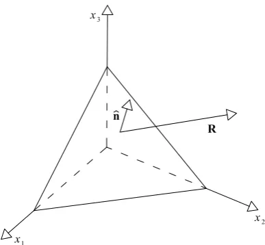
The first terms that we analyze are the stress tensors. A generic tensor can be decompose in an isotropic part plus a deviatoric one. In this way the stress tensors Ti _{(where the superscript irefers to the phases involved: f for} fluid phase and s for solid one) is decomposed in isotropic pressure pi_{I and} in tangential stresses (the deviatoric part) ¯τi _as

1.5 Closure relations 25

where I is the identity matrix. These decomposition introduces two addi-tional unknown: the solid an fluid pressure (ps _{and p}f_{), however the} intro-duction of them allows some important considerations that will be presented in the next Chapter where the shallow flow approximation is introduced.

The second important term that need attention is the interphase forces vector FF−S. From a physical point of view, this term is composed of all the forces that the fluid and the solid phases exchange each other. They are essentially the buoyancy (since there are solid particles immersed in a fluid) and the drag effect (due to possible differences of velocity between the phases). Other forces could also be introduced (e.g. the virtual added mass) but they are smaller than the first two, so we neglected them. Following the works of Armanini [7, 8] and Jackson [36], the interphase force can be decomposed as

F_iF−S =c ∂ ∂xj

T_ijf +F_iD (1.67)

where FD

i is the i-th component of the drag vector force FD, and using equation (1.66) it becomes

F_iF−S =−c ∂ ∂xi

pf +c ∂ ∂xj

τ_ijf +F_iD (1.68)

The drag force is a function of the difference between fluid and solid velocity, the net area of the particles and the density of the fluid phase

FD ∝r2ρf(uf −uS)2 (1.69)

In this way the interphase force is no more unknown since it is a function of the other unknowns of the problem.

of equations (1.64) that describe a two phase flow becomes



             

             

∂

∂t(1−c) +∇ ·((1−c)uf) = 0 ρf

∂

∂t((1−c)uf) +∇ ·((1−c)ufuf)

=−(1−c)∇pf₊ + (1−c)∇ ·¯τF _−FD _{+ (1−c)ρ}

fg

∂c

∂t +∇ ·(cus) = 0 ρs

∂

∂t(cus) +∇ ·(cusus)

=−∇ps_−c∇pf _{+∇ ·¯τ}S₊ +c∇ ·τ¯f _+FD _+cρ

sg

(1.70)

Chapter 2

The shallow flow approximation

The thee dimensional continuum equations derived in Chapter 1 compose a system that is particularly complicated and, as written in Section 1.5, requires lots of closure relations not always available in the literature. Since in a debris flow the planar scale is commonly larger than the vertical one, it is possible to introduce the shallow flow approximation which is widely used in the field of free-surface flow when this difference between the spatial scales is present. The use of the shallow flow simplification allows us to reduce the complexity of the original set of equations obtaining a simplified three dimensional system of partial differential equations which will be depth integrated later on.

2.1

Debris flow characteristic scales

With shallow flow (SF) we define a free-surface flow where the vertical scale

H is small if compared with the planar scale L

H L (2.1)

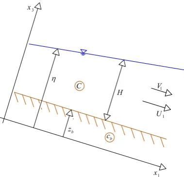
The first step, for the introduction of the shallow flow approximation, is the definition of the reference system. The choice, widely used in the derivation of the SF models, is to define the reference system (x1, x2, x3)

with the 1st _{and 2}nd _{direction parallel to the bottom (the planar axis), while} the 3rd _{one is perpendicular to it (normal direction) (see Figure 2.1).}

Figure 2.1: Sketch of the reference system and the angle of inclination α

respect the gravity force.

Usually a debris flow happens in small basins with an area of less than 5 km2 _{(see for example [44]), and has a planar extension of about hundreds}

2.1 Debris flow characteristic scales 29

• Planar directionx1 and x2 is about hundreds of meter and the

charac-teristic scale is L

L∼102 m (2.2)

• Normal direction x3 is meters with scaleH

H ∼100 m (2.3)

• Longitudinal solid (us

1, us2) and fluid velocities (u

f

1, u

f

2) have scale U

and their order of magnitude is few meters per second

U ∼100 m/s (2.4)

We use the same velocity scale for both solid and fluid phases since in an uniform flow the two velocities are similar.

• Solid (c) and liquid (β) volumetric concentrations assume different val-ues. Usually a debris flow flow has concentration of about 0.3÷0.5, so the characteristic scale is

C ∼10−1 (2.5)

on the contrary, the liquid concentration, since β = 1−c, is about 0.5÷0.7 so the same order of magnitude can be used

B ∼10−1 (2.6)

Of course the concentration of a debris flow could be larger, reaching the maximum value of around 0.65 that is the maximum concentration of the solid fraction in the bed, however here we are speaking of order of magnitude, so this approximation cold be reasonable if we look at the average over a flow event.

• Density of fluid phase ρf, that usually is water or water with silt, is about 1000 ÷1500 kg/m3 _{while the density of the solid phase ρ}

s is about 2600 kg/m3_{. The order of magnitude of the density is therefore}

• Gravity force g that must be decomposed along x3 and along x1 and

x2. Defining α as the angle between the gravity vector an the normal

to the bed (see Figure 2.1 for a sketch), the two components of the gravity are g3 =gcosα and g1 =g2 =gsinα where g is the module of

the gravity force with a characteristic scale

G∼101 m/s2

The angle α assumes different value along the path of the debris flow, ranging from 0◦ up to 20◦ and over in the triggering area. However, since we are speaking of order of magnitude we can assume an average value along the debris flow path of about 8◦÷10◦_{. With these definitions}

the two characteristic scales needed are respectively for gravity force normal to the bed and for the tangential one:

GN ∼101 m/s2 (2.8)

GT ∼10−1 m/s2 (2.9)

• The fluid pressure pf could be assumed as hydrostatic obtaining, as order of magnitude

Pf =ρGNH ∼104 P a (2.10)

• The components of the tangential fluid stresses τ_ijf with i, j = 1,2,3 can be estimated using empirical relation derived for the uniform flow such as the Gaukler-Stickler relation (see [6] for more details on this formulation)

τ0 =

ρgu2 k2

sh1/3

where ks is the Stickler coefficient with a magnitude of 101 m1/3s−1, h is the flow depth anduis the flow velocity. With this relation the order of magnitude for the components of the tangential fluid stresses is

2.1 Debris flow characteristic scales 31

• The solid pressure ps _{can be assumed hydrostatic like the fluid one.} The difference, respect to the fluid pressure, is that now we introduce the solid concentration in order to take into account the fact that not all the volume is occupied by the solid phase.

Ps=ρCGNH ∼103 P a (2.12)

Of course it is an approximation since the solid pressure, as the solid stress tensor, takes into account also the presence of the collision be-tween the particles.

• The order of magnitude for the components of solid stress tensor τ_ijs

with i, j = 1,2,3 can be estimated following the works of Armanini [8, 7] and Armanini et al. [11] where the kinetic gas theory is applied to the liquid-granular flows. Omitting all the formulation, due to its complexity and length, the final result is

Ts∼101 P a (2.13)

Among these variables are missing the time and the vertical fluid and solid velocities. In order to evaluate their orders of magnitude, it is necessary to use the first and the third equations of system (1.70) that represent the mass balances for the fluid and solid phases

∂ ∂tβ+

∂ ∂x1

βuf₁ + ∂

∂x2

βuf₂ + ∂

∂x3

βuf₃ = 0 (2.14)

∂ ∂tc+

∂ ∂x1

cus₁+ ∂

∂x2

cus₂+ ∂

∂x3

cus₃ = 0 (2.15)

The order of magnitude of one term for each equations, using the previous characteristic scales, is

∂ ∂x2

βuf₂ BU L ∼10

−3 _s−1 _(2.16)

and

∂ ∂x2

cus₂ CU L = 10

Since all the terms involved in the mass balance have the same order of magnitude, it is possible to write the following relations

B

T =

BV H =

BU L ∼10

−3 _s−1 _(2.18)

and

C T =

CV H =

CU L ∼10

−3 _s−1 _(2.19)

where T is the characteristic time scale and V is the fluid and solid normal velocity scale. From these expressions it is possible to evaluate the order of magnitude for the solid and liquid vertical velocity (us

3 and u

f

3)

V = H

LU ∼10

−2 _{m/s (2.20)}

and for the time scale T T = L

U = H V ∼10

2 _{s (2.21)}

The last term missing is the drag forceFD. As specified in equation (1.69) in Section 1.5, the drag force is a function of the difference between solid and fluid velocities, the area of the particles and the fluid density

F_iD ∝r2uf_i −us_i

2

ρf i= 1,2,3 (2.22)

In order to understand the order of magnitude of the these forces, we assume that the radius of the particles is about 10−1 _{m, while the maximum difference}

between the two velocity is reached when the solid particles are stationary and the fluid is moving (this happens in the triggering and deposition area where the debris flow starts and stops) so uf_i −us_i

2

∼ uf_i

2

with i = 1,2,3. With these assumption the order of magnitude for the drag force on direction

i= 1,2 is

F_TD ∼101 N (2.23)

while for the normal direction i= 3 becomes

2.2 Simplification of the momentum equations on the normal direction 33

We want to highlight that this is only an order of magnitude for the drag force valid in the triggering and deposition area where the solid velocity is null. Instead, when the uniform flow is developed the fluid and solid velocities have the same order of magnitude, so the drag force becomes negligible. Since we are speaking about the orders of magnitude, we can assume that the drag force values obtained are also the same when we refer to a unit volume, so we can use them inside the momentum equations.

An estimation of the magnitude of all the variables present into the three dimensional equations for a continuum fluid-granular mixture flow derived in Chapter 1 are presented, so it is possible to evaluate which terms into these equations can be neglected under the shallow flow approximation.

2.2

Simplification of the momentum equations

on the normal direction

The first equation we analyze is the momentum balance for the fluid phase along the normal direction that is the second equation of system (1.70). Expanding all the terms, the equation reads

∂ ∂tβu

f

3 +

∂ ∂x1

βuf₁uf₃ + ∂

∂x2

βuf₂uf₃ + ∂

∂x3

βuf₃uf₃ = =−β

ρf

∂ ∂x3

pf + β

ρf

∂ ∂x1

τ₁₃f + β

ρf

∂ ∂x2

τ₂₃f + β

ρf

∂ ∂x3

τ₃₃f − F D

3

ρf

+βg3

(2.25)

all the terms are expressed in m/s2₎ ∂ ∂tβu f 3 BV T = 10

−1 _; ∂

∂x1

βuf₁uf₃ BU V L = 10

−5

∂ ∂x2

βuf₂uf₃ BU V L = 10

−5 _; ∂

∂x3

βuf₃uf₃ BV

2

H = 10

−5

β ρf

∂ ∂x3

pf BP

f

ρH = 10

0 _; β

ρf

∂ ∂x1

τ₁₃f BT

f

ρL = 10

−4

β ρf

∂ ∂x2

τ₂₃f BT

f

ρL = 10

−4 _; β

ρf

∂ ∂x3

τ₃₃f BT

f

ρH = 10

−2

F₃D ρf

F_ND ρ = 10

−6 _{; βg}

3 GN = 100

Taking into account only the terms with the highest order of magnitude (so 100_{) the fluid momentum equation in the normal direction becomes}

−β

ρf

∂ ∂x3

pf +βg3 = 0 (2.26)

which, simplifying β, becomes

∂ ∂x3

pf =ρfg3 (2.27)

The starting solid phase momentum equation along the normal direction is the fourth equation in system (1.70) that reads

∂ ∂tcu s 3+ ∂ ∂x1

cus₁us₃+ ∂

∂x2

cus₂us₃+ ∂

∂x3

cus₃us₃ = = F

D

3

ρs

+cg3 +

1

ρs

− ∂

∂x3

ps−c ∂ ∂x3

pf + ∂

∂x1

τ₁₃s + ∂

∂x2

τ₂₃s + + ∂

∂x3

τ₃₃s +c ∂ ∂x1

τ₁₃f +c ∂ ∂x2

τ₂₃f +c ∂ ∂x3

τ₃₃f

(2.28)

2.2 Simplification of the momentum equations on the normal direction 35

of the different terms into this equation are

∂ ∂tcu

s

3

CV T = 10

−1 _; ∂

∂x1

cus₁us₃ CU V L = 10

−5

∂ ∂x2

cus

2us3

CU V L = 10

−5 _; ∂

∂x3

cus

3us3

CV2

H = 10

−5

1

ρs

∂ ∂x3

ps P s

ρH = 10

0 _; 1

ρs ∂ ∂x1 τs 13 Ts

ρL = 10

−4

1

ρs

∂ ∂x2

τ₂₃s T_ρLs = 10−4 ; 1

ρs

∂ ∂x3

τ₃₃s T

s

ρH = 10

−2

c ρs

∂ ∂x3

pf CP

f

ρH = 10

0 _; c

ρs

∂ ∂x1

τ₁₃f CT

f

ρL = 10

−4

c ρs

∂ ∂x2

τ₂₃f CT

f

ρL = 10

−4 _; c

ρs

∂ ∂x3

τ₃₃f CT

f

ρH = 10

−2

F₃D ρs

F_ND ρ = 10

−6 _{; cg}

3 CGN = 100

Using only the first order of approximation, so neglecting all the term with a magnitude less than 100_{, the solid momentum equation along thex}

3 direction

reduce to

∂ ∂x3

ps+c ∂ ∂x3

pf =cρsg3 (2.29)

The normal derivative of both solid and liquid pressures appears in this equation. However, using equation (2.27) that describe the normal derivative of the fluid pressure, equation (2.29) becomes

∂ ∂x3

ps = c(ρs−ρf)g3

= cρ0g3 (2.30)

and represent the vertical variation of the solid pressure, whereρ0 = (ρs−ρf) is the submerged solid density.

2.3

Simplification of the momentum equations

on the planar direction

The momentum equation in the plane x1, x2 for the fluid phase derived in

Section 1.4 is

∂ ∂tβu f i + ∂ ∂x1

βuf₁uf_i + ∂

∂x2

βuf₂uf_i + ∂

∂x3

βuf₃uf_i = =−β

ρf

∂ ∂xi

pf + β

ρf

∂ ∂x1

τ₁f_i+ β

ρf

∂ ∂x2

τ₂f_i+ β

ρf

∂ ∂x3

τ₃f_i−F D i

ρf

+βgi (2.31)

where i= 1,2.

The order of magnitude of each terms in this equation, using i = 1, are the same than using i = 2 since these two directions are, up to now, interchangeable. The magnitude of these terms are the following

∂ ∂tβu

f i

BU T = 10

−3 _; ∂

∂x1

βuf₁uf_i BU

2

L = 10

−3

∂ ∂x2

βuf₂uf_i BU

2

L = 10

−3 _; ∂

∂x3

βuf₃uf_i BU V H = 10

−3

β ρf

∂ ∂xi

pf BP f

ρL = 10

−2 _; β

ρf

∂ ∂x1

τ₁f_i BT

f

ρL = 10

−4

β ρf

∂ ∂x2

τ₂f_i BT

f

ρL = 10

−4 _; β

ρf

∂ ∂x3

τ₃f_i BT

f

ρH = 10

−2 FD i ρf FD T

ρ = 10

−2 _{; βg}

i BGT = 10−2

Taking into account only the leading terms (so the ones with magnitude of 10−2_{) the resulting equation describe only permanent flow where no time}

variation is allowed. We remember that, as said in Section 2.1, that in a permanent flow the drag term is smaller, so it is negligible. Since we want to study phenomena with a time variation in the plane, we need to take into account also the term with an order of 10−3_{. With this approximation it is}

2.3 Simplification of the momentum equations on the planar direction 37

flow approximation, for a two-phase