DEPARTMENT OF INFORMATION ENGINEERING AND COMPUTER SCIENCE ICT International Doctoral School
Distributed computing for
large-scale graphs
Models, Algorithms, Applications
Alessio Guerrieri
Advisor
Prof. Alberto Montresor
Universit`a degli Studi di Trento
Abstract
The last decade has seen an increased attention on large-scale data analysis, caused mainly by the availability of new sources of data and the development of programming model that allowed their analysis. Since many of these sources can be modeled as graphs, many large-scale graph processing frameworks have been developed, from vertex-centric models such as pregel to more complex programming models that allow asynchronous
computation, can tackle dynamism in the data and permit the usage of different amount of resources.
This thesis presents theoretical and practical results in the area of distributed large-scale graph analysis by giving an overview of the entire pipeline. Data must first be pre-processed to obtain a graph, which is then partitioned into subgraphs of similar size. To analyze this graph the user must choose a system and a programming model that matches her available resources, the type of data and the class of algorithm to execute.
Aside from an overview of all these different steps, this research presents three novel approaches to those steps. The first main contribution isdfep, a novel distributed
parti-tioning algorithm that divides the edge set into similar sized partition. dfep can obtain
partitions with good quality in only a few iterations. The output of dfep can then be
used by etsch, a graph processing framework that uses partitions of edges as the focus
of its programming model. etsch’s programming model is shown to be flexible and can
easily reuse sequential classical graph algorithms as part of its workflow. Implementations of etsch in hadoop,spark and akkaallow for a comparison of those systems and the discussion of their advantages and disadvantages. The implementation ofetsch inakka is by far the fastest and is able to process billion-edges graphs faster that competitors such as gps, blogel and giraph++, while using only a few computing nodes. A final contribution is an application study of graph-centric approaches to word sense induction and disambiguation: from a large set of documents a word graph is constructed and then processed by a graph clustering algorithm, to find documents that refer to the same enti-ties. A novel graph clustering algorithm, namedtovel, uses a diffusion-based approach
inspired by the cycle of water.
Keywords
Contents
I Introduction to Large-scale Graph Analysis 1
1 Introduction 3
2 Sources of Graphs 5
2.1 Large-scale graphs . . . 6
2.2 Sources of graphs . . . 7
2.3 Characteristics of graphs . . . 8
3 Systems for Graphs Analysis 11 3.1 Motivations for large-scale graph processing systems . . . 11
3.2 Requirements for graph processing systems . . . 13
3.3 Choosing a large-scale graph processing system . . . 14
4 Problems and applications on graphs 15 4.1 Customer of the application . . . 15
4.2 Timing of the application . . . 16
4.3 Computation on or about graphs . . . 17
4.4 Types of approaches . . . 17
II Foundations of Graph Analysis 19 5 Building the Graph 21 5.1 Graphs from clean data . . . 21
5.2 Graphs from dirty data . . . 22
5.3 Graphs from crawls . . . 22
5.4 Indices of graphs . . . 23
6.2 Introduction to graph partitioning . . . 26
6.3 Formal definitions . . . 27
6.4 Advantages of edge partitioning . . . 29
6.5 Approaches to graph partitioning . . . 30
6.5.1 Quick heuristic partitioning . . . 31
6.5.2 Specialized partitioning . . . 32
6.5.3 Partitioning via exchanges . . . 32
6.5.4 Multi-level partitioning . . . 33
6.5.5 Streaming partitioning algorithms . . . 33
6.5.6 Distributed partitioning . . . 35
7 DFEP: Distributed Funding-based Edge Partitioning 37 7.1 Distributed Funding-based Edge Partitioning . . . 37
7.1.1 Variants and additions . . . 42
7.2 Results . . . 42
7.2.1 Metrics . . . 43
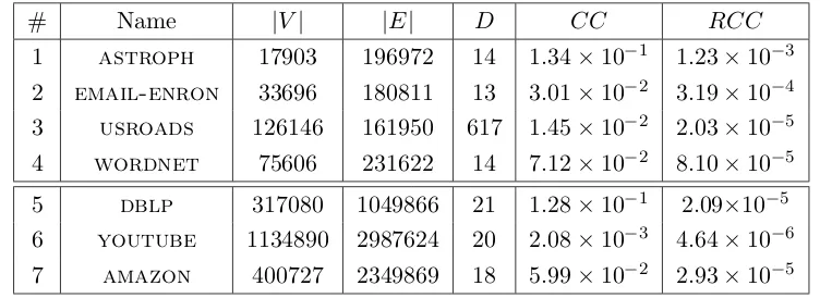
7.2.2 Datasets . . . 43
7.2.3 Simulations . . . 44
7.2.4 Experiments in EC2 . . . 48
7.3 Future work . . . 48
III Computation on Large-scale Graphs 51 8 Graph Processing Systems 53 8.1 Pregel and Giraph . . . 53
8.2 GraphLab and GraphX . . . 57
8.3 Partition-centric frameworks . . . 59
8.4 Low-memory frameworks . . . 61
8.5 Frameworks for dynamic graphs . . . 62
8.6 Frameworks for asynchronous computation . . . 63
8.7 Graph databases . . . 64
8.8 Other frameworks . . . 65
9 ETSCH: Partition-centric Graph Processing 67 9.1 Introduction . . . 67
9.2 ETSCH . . . 68
9.2.2 Applicability of Etsch . . . 73
9.2.3 Partitioning schemes . . . 74
9.3 Results . . . 75
9.3.1 Datasets . . . 75
9.3.2 Hadoop . . . 76
9.3.3 Spark . . . 76
9.3.4 Akka . . . 77
9.3.5 Comparison with Blogel and GPS . . . 79
9.4 Conclusions . . . 80
IV Applications of Large-scale Graph Analytics 83 10 Applications of Graph Processing 85 10.1 Strategies . . . 85
10.2 Overview of graph problems . . . 87
10.2.1 Triangle counting . . . 87
10.2.2 Centrality measures . . . 88
10.2.3 Path computation . . . 89
10.2.4 Coloring . . . 90
10.2.5 Subgraph matching . . . 91
11 Graph Clustering for Word Sense Induction 93 11.1 Problem statement . . . 94
11.2 Related work . . . 95
11.2.1 Word sense induction and disambiguation . . . 95
11.2.2 Graph clustering . . . 96
11.3 Graph construction . . . 97
11.4 Tovel: a Distributed Graph Clustering Algorithm . . . 98
11.4.1 Data structures . . . 99
11.4.2 Main cycle . . . 99
11.4.3 Convergence criterion . . . 102
11.4.4 Rationale . . . 102
11.5 Analysis . . . 103
11.5.1 Quality at convergence . . . 103
11.5.2 Sizes at convergence . . . 104
11.5.3 Computing pour for word sense induction . . . 105
11.7 Experimental results . . . 107 11.8 Future work . . . 109
V Concluding Remarks 111
12 Conclusions 113
Publications 115
Bibliography 117
List of Tables
3.1 Timeline of events . . . 13
6.1 Terminology of different definitions of partitioning . . . 29
7.1 Notation . . . 39
7.2 Datasets used in the simulation engine (1-4) and EC2 (5-7) . . . 44
8.1 Overview of frameworks introduced in this chapter. For each framework, we list the programming model, the type of resources used by the framework, if it allows for asynchronous execution and if it can cope with dynamism in the graph . . . 54
9.1 Datasets used with etsch/hadoopand etsch/spark . . . 76
9.2 Datasets used with etsch/akka . . . 76
9.3 Comparing different frameworks for etsch, using 4 machines. . . 79
9.4 Comparison of running time of a single PageRank iteration inetsch, blo-gel, gps(8 m3.largemachines) . . . 80
11.1 Simple example: 4 documents, Apple is the target ambiguous word with two different senses (the fruit and Apple Inc.) . . . 94
11.2 Notations used in the analysis of tovel (Section 11.5) . . . 103
11.3 Datasets used in evaluation . . . 107
List of Figures
2.1 Structure of the World Wide Web graph, from Graph Structure in the
Web [24] . . . 7
6.1 Degree distribution of a) actor collaboration graph b) world wide web graph and c)powergrid data, from [14]. Each of these graphs follows a different power-law degree distribution . . . 26
6.2 Vertex partitioning example: each vertex appears in one partition, cut edges connect partitions . . . 27
6.3 Edge partitioning example: each edge appears in only one partition, while frontier vertices may appear in more than one partition . . . 28
6.4 On the left, a graph with labels on the edges. On the right, its line graph. For each edge in the original graph a new vertex is created. Two vertices are connected if, in the original graph, the corresponding edges had a node in common . . . 30
6.5 Illustrative scheme of multilevel partitioning algorithms, from http:// masters.donntu.org/2006/fvti/shepel/diss/indexe.htm . . . 34
7.1 Sample run of Step 1 and 2 of dfep . . . 40
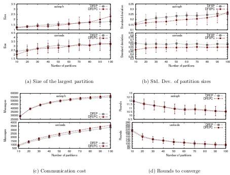
7.2 Behavior of dfep and dfepc with varying values of K . . . 45
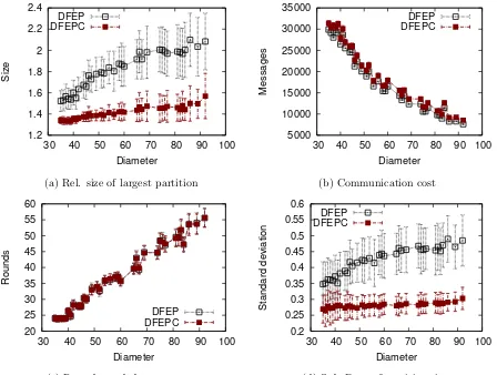
7.3 Behavior of dfep and dfepc with varying diameter (K = 20) . . . 46
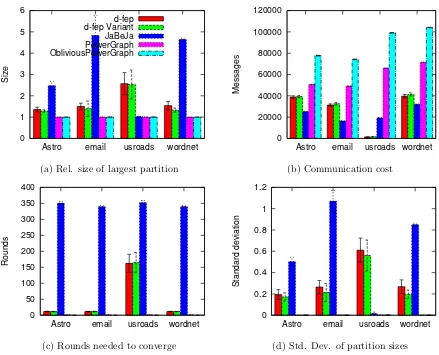
7.4 Comparison between dfep, dfepc, ja-be-jaand Powergraph’s greedy partitioning algorithm (K = 20) . . . 47
7.5 Speedup of real implementation of dfepin Amazon EC2 . . . 49
8.1 Vertex’s state machine in pregel (from [70] . . . 55
8.2 Sample run of max-number computation in pregel. Gray vertexes are inactive. (from [70] . . . 55
9.1 Example of vertex and edge partitioning: on the top figure, vertices are partitioned and a few cut edges connect vertices belonging to different partitions. On the bottom figure, edges are partitioned and a few frontier vertices appear in more than one partition . . . 69 9.2 Illustrative schema of etsch . . . 70
9.3 Running time of single source shortest path algorithm in hadoop
compar-ing a standard baseline algorithm and etsch, withm3.largemachines on EC2. . . 77 9.4 Comparison between etsch and the standard pregel implementation in
spark/graphx . . . 78
9.5 Scalability of etsch/akka on the larger datasets, using m3.large ma-chines on EC2. For each experiment we measure the average time for a complete iteration of PageRank . . . 80 11.1 Sample graph created from Table 11.1. Blue nodes are ambiguous. . . 98 11.2 Illustration of the water cycle in tovel . . . 102
11.3 Average color per node in a cluster at steady state, for different quality and values of pour, in a graph with 1000 nodes . . . 105
Part I
Introduction to Large-scale Graph
Chapter 1
Introduction
To a person who has studied extensively the concept of graphs and their possible ap-plications, recognizing graphs in nature becomes trivial. Graphs can represent relations between people, show connections between places, track the spreading of ideas and the interaction between molecules. As people we daily build a network of friendship and relations, follow a network of routes to meet these people and make all these decisions through a network of neurons in our brain. Once you learn to see graphs, you recognize them everywhere.
It may be a surprise then noticing that the concept of graphs is relatively new. Euler used graphs to prove the impossibility of a solution to the Seven Bridges of Koenigsberg problem in 1736 [33], but this concept did not have a name until Sylvester in 1878 used the term ”graph” for the first time [109]. In the following decades mathematicians were stimulated by problems such as the four-color problem and the graph enumeration prob-lems, but the field did not start studying real-world graphs in depth before the advent of computer science.
Until only a few decades ago, computer science was pursuing research in more efficient graph algorithms, but the number of real-world graphs that needed to be analyzed was still small. Most research was on problems related to computer networks, such as routing and congestion detection, and problems on geographical graphs, such as path computation.
CHAPTER 1. INTRODUCTION
algorithms.
Chapter 2
Sources of Graphs
One of the latest trend in computer science is the emergence of the “big data” phe-nomenon that concerns the retrieval, management and analysis of datasets of extremely large dimensions, coming from wildly different settings. For example, astronomers need to examine the huge amount of observations collected by the new telescopes that are being built both on Earth and in orbit [49]. Biological experiments create large genomic and proteinomic datasets that need to be processed and understood to reach new break-throughs in the study of drugs [51]. Governments can improve the quality of life of their citizens by analyzing the huge collections of individual events related to traffic, economy, health-care and many other areas of everyday life [48]. The scale of such datasets keeps increasing exponentially, moving from gigabytes to terabytes and now even to petabytes.
Several interesting datasets are structured in a way that makes them easy to be mod-eled as graphs with additional information labeling vertices and edges. An obvious exam-ple is the World Wide Web, but there are many other examexam-ples such as social networks, biological systems or even road networks. While graph problems have been studied since before the birth of computer science, the sheer size of these datasets makes even classic graph problems extremely difficult to solve. Computing the shortest path between two nodes needs too many resources to complete in time when the graph is too big to fit into memory.
CHAPTER 2. SOURCES OF GRAPHS
2.1
Large-scale graphs
Before discussing how to run our analysis and the information that we want to obtain from this data, we need to understand what are large-scale graphs and where do they comes from. While there are many different definition of what is “Big Data”, most agree on the 3V model [64]: a problem is “Big Data” when the volume of data, the velocity of its changes or the variety of its data makes it impossible to use traditional data processing algorithms and systems.
Trying to apply this definition in large-scale graph processing allow us to get some intuition on the particularity of this area of research inside the more general “Big Data” field. The issue of variety becomes less crucial since we are restricting the datasets to those that can be represented as graphs, while the issue of volume becomes more interesting since it could refer to both the size of the graph or the amount of data associated to it.
We can adapt the classical “Big Data” definition to say that there is a need of a large-scale graph processing approach when:
• The size of the graph has become too large: storing the vertices and edges in memory is an issue and the complexity of traditional algorithms makes them impractical for graph of this scale.
• The amount of data on the graph, such as information associated to vertices and edges, has become too large.
• The data is changing too quickly, because of addition and deletion of vertices and edges or continuous updates to the states of both.
From the 3V model we removed the Variety requirement and split the Volume re-quirement in two, differentiating between the graph itself and the information on top of it. Computing a centrality metric such as PageRank on a small graph can be easily completed using traditional techniques; when the graph grows larger, however, it becomes costs-ineffective to use just a single machine. For traffic analysis on road networks the vol-ume issue is much different: the graphs will typically be relatively small, but the amount of information associated to them, such as the load of each street at different times of day, can be so huge it makes traditional approaches unusable.
2.2. SOURCES OF GRAPHS
Figure 2.1: Structure of the World Wide Web graph, from Graph Structure in the Web [24]
2.2
Sources of graphs
While the Variety requirement is not as important as in the general “Big Data” setting, large-scale graphs can come from different type of sources that determine some of their characteristics. Most graphs represent activity and connections between entities (be it people or more abstract concepts) and therefore are very dynamic. Only in a few cases the large-scale graphs represents mostly static real-world connection patterns.
CHAPTER 2. SOURCES OF GRAPHS
are generated by all the users of the Web, but they might come with privacy issues, since they reflect possible private activity by real people. Note that even if in most cases edges and nodes are added to the graph incrementally and there might be information about timestamps of these events, the graphs are often considered as static and the timing information is simply discarded once the new nodes and edges are added to the graph.
A smaller amount of graphs come from activity of people and other entities in the real world, such as connections extracted from news, government documents or sensors deployed in the world. These datasets are not as clean as the ones coming from activity on the web, since they must be digitalized and pre-processed to extract the information needed. While in social networks there is a unique id for each person, in the real world the task of understanding which people does a document refers to becomes a challenging task by itself. Another consequence of this obstacle is that the amount of data that goes through this pipeline to reach the graph analysis computation is much smaller than in the other cases. Problems on graphs coming from these sources can still be considered “Big Data” if the amount of computation is really heavy, but in many cases only the pre-processing phase (such as the text entity recognition) is properly Big Data, while the graph processing could be done using more traditional techniques. Privacy is even more a concern, especially in cases in which the graph regards flow of money or movement tracking.
Finally, there a few graphs that refer to existing structures in the real world. While a social network can be seen as an extension of the real societal network, here we con-sider more physical graphs such as road networks, biological networks, food networks and similar systems. These are usually very small (in comparison with other networks) and also not easy to obtain and build. What makes these graphs “Big Data” is the amount of information that often is connected to vertices and edges in these systems. For example, road networks are small, but traffic analysis on those road networks require heavy com-putation and massive quantities of data. In most cases privacy concerns are less heavy in these networks, since their real world counterparts are publicly available.
Almost all applications that are explored in this thesis come from the first two cate-gories, while analysis of physical graphs is used just to show the impact of their charac-teristics on their analysis.
2.3
Characteristics of graphs
2.3. CHARACTERISTICS OF GRAPHS
scenario, the source will continuously send data across the pipeline and both systems and algorithms will have to adapt to it. While it is possible to process dynamic graphs with static tools, it becomes infeasible when either the flow of data is too fast or the problem is time critical and delays in updating the result can be damaging.
Note that temporal graph analysis, in which an algorithm uses or studies the changes in shape of the graph through time, can be both static and dynamic. Often changes to such graphs are not that quick to force the use of dynamic techniques and the analysis can be run again from scratch whenever the application needs an updated result, but that is not always the case.
Another distinction is between homogeneous or heterogeneous graphs. Co-purchasing networks, graphs that contain information about which products are purchased together, can be stored in both ways. In an homogeneous network each node will represent a product and there will be an edge between two products if they have been purchased by the same user. In an heterogeneous network nodes can be either products or users, while edges will connects users and their purchases. This graph is heterogeneous because the nodes are not all of the same class of entity and will thus have completely different types of data associated to them.
Chapter 3
Systems for Graphs Analysis
The data analysis field has reacted in different ways to the growth in size of available datasets. As the new architectures have shown a reduced interests in faster and faster CPUs and have and focused on efficient multi-core architectures, the parallelism of the analysis has also become a crucial characteristic.
While parallel (multi-CPU, multi-core) systems have been used to deal with this deluge of data, there are many cases in which distributed approaches are the only viable road. The disadvantages of distribution cannot be ignored, though: distributed algorithms are inherently more difficult to develop and implement, and they bring a larger communication overhead. Nevertheless, the advantages outweigh the disadvantages. A distributed system is able to cope with potentially unlimited datasets, is more robust to hardware failures, is often cheaper and, with the emergence of distributed frameworks for data analysis, is also much easier to use than it was a decade ago. These new distributed frameworks abstract away most of the challenges of building a distributed system and offer the analysts straightforward programming models for their data analysis programs.
This chapter illustrates the underlying reasons for this proliferation of large-scale graph processing frameworks both in academic and industrial settings, and introduces the dif-ferent types of framework and their difdif-ferent approaches.
3.1
Motivations for large-scale graph processing systems
The immense growth in number and complexity of large-scale graph analysis frameworks can be explained not only by the availability of data but also by the challenges posed by the analysis of these graphs.
CHAPTER 3. SYSTEMS FOR GRAPHS ANALYSIS
obtain outgoing edges of a single node, follow those edges and recover or update data associated with those nodes or edges. Classical approaches, such as the commonly used adjacency lists, can be extremely inefficient when the size of the graph is so large that every byte of memory is important.
These challenges become even more harsh when you need to cope with multiple threads, multiple processes or even multiple machines that are trying to access the graph. Writing a system that can solve all those problems and is flexible enough to not be limited to a single algorithm is not a task that users will want to tackle, if also given access to a readily prepared framework.
Another very important factor for the proliferation of graph processing framework has been the fact that the development of these framework did not necessarily have to start from scratch. In many cases they were created as a tools inside already existing ecosystems, along side other “Big Data” tools. hama [102] and giraph [8] started as part of the hadoop [16] ecosystem, graphx [121] was born by adding graph-specific
code to spark[124] and gellyas an extension of flink[5]. On the developers side, this
opportunity made it possible to reuse already available tools and start from an already existing user base. The users were more likely to test these frameworks if they had previous experience with the ecosystem and were allowed to combine standard machine learning techniques with graph analysis algorithms and obtain data pipelines impossible in stand-alone graph frameworks. One of the main selling points of spark has been the fact that
users could get data, clean it, pre-process it, create a graph, run a graph algorithm and finally obtain the output all in one program, without having to leave the ecosystem.
The only extremely successful standalone graph processing framework,graphlab[68],
also stopped being standalone just when it had reached maturity. To widen the scope of the project, the developers kept the extremely efficient core of graph analytics and reused many techniques to build a generic machine learning oriented framework around it. This choice could signal that in the future, the place of distributed graph processing framework will be inside larger ecosystems and the competition will be between the ecosystems that host the frameworks, not on the framework themselves.
Interestingly, this pattern has not been necessarily true for non-distributed graph databases, where standalone frameworks such as neo4j[78], OrientDB[83] or Spark-See [105] continue to thrive. The most likely reason for these exception is the lesser need
3.2. REQUIREMENTS FOR GRAPH PROCESSING SYSTEMS
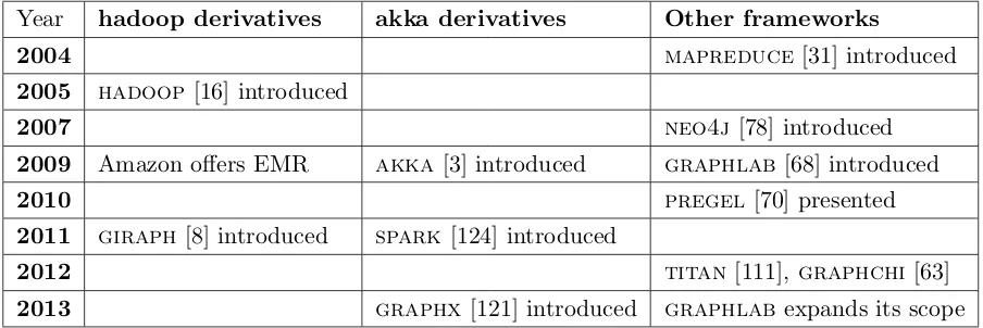
Table 3.1: Timeline of events
Year hadoop derivatives akka derivatives Other frameworks
2004 mapreduce [31] introduced
2005 hadoop[16] introduced
2007 neo4j[78] introduced
2009 Amazon offers EMR akka[3] introduced graphlab [68] introduced
2010 pregel [70] presented
2011 giraph [8] introduced spark[124] introduced
2012 titan [111], graphchi[63]
2013 graphx[121] introduced graphlab expands its scope
3.2
Requirements for graph processing systems
Before starting to differentiate these systems, we can start by looking at what is requested by the users. In this section we consider clients both the cluster administrators (that need to run the system on their cluster) and the programmers that use the system.
The core concept that all these systems have to take in mind is the idea that in the “Big Data” scenario efficiency is less important than manageability. In clusters with thousands of nodes and petabytes of data, efficiency is still important but secondary to the assurance that the computation will continue and data will not be lost even in presence of hardware failures in the system. Since failures are virtually guaranteed to appear, being resilient to failures is actually the most important feature of a large-scale distributed system.
A second, important property of a successful system is the ease of use of both its interface to the programmer and its interface to the administrator. The programming model should allow different levels of abstraction, to give satisfaction to programmers with different skill levels. On the administrator side, these systems should be as predictable as possible, to allow for accurate estimation of costs and time spent on different analysis.
CHAPTER 3. SYSTEMS FOR GRAPHS ANALYSIS
3.3
Choosing a large-scale graph processing system
Considering the wide range of sources of graphs and applications, it is not a surprise to find that graph processing frameworks can be immensely different from each other. To find a pattern, it is necessary to study three different factors: resources, data and algorithms.
The type of resources available to the user is the biggest motivator in deciding which framework to use. From less powerful to more powerful, frameworks can target commod-ity level machines, shared-memory clusters and distributed systems. While it might seem counter-intuitive to create a “Big Data” framework and run it on a single cheap machine, forward-looking users might decide to adopt the framework at very early stages of devel-opment to make sure that they will be able to scale to larger quantity of data by simply upgrading the hardware and not changing the software. Having an efficient, small-scale implementation can also increase the visibility of the framework. As an example, the
SparkSee graph databases not only claims to be extremely efficient on shared-memory
clusters, but also the first graph database for Android, in the hope of gaining visibility from mobile developers. While there are similarities between frameworks for commodity-level machines and shared-memory clusters, frameworks for distributed systems tend to be extremely different in structure and technology because of the need of distributed file systems and message passing architectures. While distributed systems can be run on single machines, in that setting they can be useful only to develop and test the programs that will be eventually run on a large clusters.
Another important factor in choosing the right system is the type of data that the user needs to analyze. Frameworks can focus on RDF data or generic graph data. While RDF is usually represented by subject-predicate-object triples, generic graphs can con-tain additional data inside vertices or edges and therefore is more difficult to fit into a specialized system for RDF analysis.
Chapter 4
Problems and applications on graphs
It is impossible to categorize all possible applications of large-scale graph analysis, but there are some patterns that can be evinced from how these systems are used in the industry. The best indicators for understanding which type of application are (i) who is the computation for (who will use its output); (ii) how quickly is an answer needed; (iii) whether it is directly a graph problem or a problems that needs the use of graphs; finally, (iv) the type of solution that this problem will need. As is shown in this chapter, all these properties influence each other and can be important factors in the choice of system to tackle the problem.
4.1
Customer of the application
The first important factor to consider is who wants the problem to be solved. In some cases, the application is just used internally by the owner of the data, without showing its results directly to the public. In other cases, the information gathered is then presented to the users and changes the way they interact with the system. A special case appears when the owner of the data is an information provider, a company which product is the information itself.
When the owner of the data needs to understand something about that data, there is seldom a question of timeliness. Unless the application uses large-scale graph processing to create an alert system, the owner will only need sporadic updates to keep track of patterns of change in the graph. Twitter might want to track the spread of influence between its users to develop better way to recommend connection to other users, but daily updates are not needed. Computing the community structure of its users (and the rate of activities of those community) can be helpful to encourage activity on the system, but it can be executed only when there is a specific need.
CHAPTER 4. PROBLEMS AND APPLICATIONS ON GRAPHS
If a user needs to know similar items to an already bought item, they cannot receive outdated information. Periodical updates to the knowledge base require the system to be run often and to keep track of new activities by the users. Another requirement appears in this scenario: this information must be either be precomputed and readily available, or computed very quickly. More than a few seconds of delay could already be not acceptable in the modern web.
These requirements becomes even more stringent if the owner of the data is an informa-tion provider. The users of these services pay for access to the output of the informainforma-tion provider’s analysis and require updated, thorough and quick answers to their query. Pre-dictability is key: if an update to the data is promised for a certain day, the information provider cannot delay it without incurring in significant costs to its image. Choosing algorithm with precise running time in stable, fault-tolerant systems becomes a priority.
4.2
Timing of the application
How quickly must an answer be given to the customer is an extremely important factor that has repercussions on all subsequent choices. There is a sliding scale that goes from real-time computation to time insensitive, batch processing.
The most demanding scenario is one in which answers are expected almost on real-time. For this scenario to appear the data must appear very quickly, either directly through interaction on the web or through sensors in the real world. Systems must typically find interesting anomalies and react quickly by alerting experts or specialized systems. This type of applications is infrequent in large-scale graph processing, especially compared with its frequency in the more general Big Data scenario. Even the example of adapting shortest route computation in case of congestion (either in road or computer networks) seldom requires an amount of computation sufficient to justify large-scale graph processing systems.
In a more relaxed scenario, where efficiency is not crucial but still very important, low-level systems are at advantage over general large-scale processing frameworks. There is a trade-off between abstraction and efficiency, therefore systems that offer pregel’s
programming model will seldom be as efficient as systems that just offer fast message passing primitives. Since every problem becomes time-sensitive if the amount of data becomes too big, using lower level primitives is a valid approach whenever more general programming models are too slow to complete the computation quickly enough.
4.3. COMPUTATION ON OR ABOUT GRAPHS
and higher stability. There are still some concerns about efficiency, since executing in less time would mean smaller costs, but they are less pressing than in other scenarios.
4.3
Computation on or about graphs
Another important factor that influences the choice of system to be used is how this application uses graphs in its computation. It can either study a graph to obtain some insight, or it can build and use a graph as a tool to highlights connection in unstructured data.
As example, computing the centrality of accounts in a social network is a problem that studies properties of a specific, already existing graph. Finding paths in such a network needs only the graph itself and does not need any steps before or after the actual graph computation.
This is not true whenever graphs are used as tools inside a larger system. Chapter 11 presents an approach that creates a network of words from unstructured documents, and clusters the resulting graph to get insight about the properties of those documents. Even simpler graphs, such as co-purchasing networks, are built from information that needs pre-processing to be seen as graphs.
The biggest consequence of this factor is the choice of a stand-alone, specialized graph processing system against a more general system that can be connected with other big data frameworks inside an ecosystem. If the application needs pre- or post-processing before and after the graph computing phase, the user might well choose a slower graph computing framework that at least lives inside a large ecosystem of big data frameworks.
4.4
Types of approaches
Even if the problem that needs to be solved is novel, it is usually the case that the developers know which type of approach they will need. Knowing if it is a problem that can be solved from local informations, from knowledge about paths or from the similarity between nodes or edges gives an indication of what type of systems the user should use.
Problems that can be solved with local information, such as queries about the degrees of nodes or finding nodes with specific characteristics can typically be solved by large-scale graph databases. RDF queries are quite powerful and modern graph databases can process these queries at a speed that would not be reachable by more general graph processing frameworks.
CHAPTER 4. PROBLEMS AND APPLICATIONS ON GRAPHS
define the position of a node by looking at the paths in which the node is involved. These problems typically needs many more iterations to converge, but often the running time depends on the diameter of the graph. On small-world graphs, such as most social interaction networks, the diameter is small enough to limit the loss of efficiency caused by having to synchronize all the machines at the start of each iteration. In cases where diameter is large there are two possible solutions: either use more specialized systems (such as frameworks for analysis of geographical graphs) or frameworks with asynchronous programming models.
Part II
Chapter 5
Building the Graph
The first step across the pipeline that connects the origin of the data to the results given to the users is the extraction and pre-processing of the graph. This process can be trivial in cases where the graph is already natively stored by the owner of the original data, but it can become a challenge by itself when the source data is unstructured, in a remote location, or is a composition of different sources.
In this Chapter we give an overview of the challenges in obtaining the data, construct-ing the graph and preparconstruct-ing for the analysis of the graph.
5.1
Graphs from clean data
In the least challenging scenario the graph is constructed from structured data owned by the analyst itself. For example, Facebook or Google might want to analyze the social network of its users or study their activity.
If the data is well-structured and the connections between the entities are already explicit in the data, then the problem is trivial. Social networks such as Facebook or Twitter have a complete view of their users and the connection between them, without any ambiguity. Networks that can be indirectly inferred from structured data, such as co-purchasing networks, can also be constructed without complications.
Challenges may arise when the analyst wants to also use unstructured data to add information to the graph. Connections in Google Plus can be grouped in circles, but the meaning of each circle (usually described by a single word) is different for each user. This problem gives a foretaste of the difficulties of building a graph in a less clean scenario.
CHAPTER 5. BUILDING THE GRAPH
to a format readable by the graph processing system.
5.2
Graphs from dirty data
While the previous setting is frequent, there are many complications that may arise when the graph must be constructed from less clean sources or if the owner of the data is not the same as the analyst.
These challenges appear most often when the analyst is using data coming from dif-ferent sources; in such cases, hoping that companies will use a common ontology to define the connections inside their data is futile. Consider, for example, the case in which two different datasets containing corporate positions of workers in companies must be inte-grated. The terminology used by the two sources to define the type of position will often be different and creating a mapping between the two terminologies to reconciliate the two datasets will be a thankless job that will be probably be assigned to a human worker.
This setting can be even more challenging when the graph is in an unstructured form, such as when a network of interactions must be extracted from text data. If we want to create an edge between two entities when they co-appear in a piece of news, the first problem to solve is understanding which sequence of words are entities. Then those entities must be mapped to the ontology used by the system, making sure to differentiate between entities that have different meaning but same text (such as people with the same name). Extracting the type of connection from the text is only the last step to obtain a well-structured and meaningful graph [77] [35].
Each of these steps can and will introduce errors in the graph. The analysts need to carefully consider the impact of these errors on their applications and if they might invalidate their results. Not all errors are equals: services that collect news regarding different companies are more worried about mistakes in the data regarding its largest users, while errors in recognizing small, local companies can be less crucial.
5.3
Graphs from crawls
Graphs can be difficult to build for an orthogonal reason: the data may be well-structured, but not directly available. If the data is distributed between different entities and is not given directly to the analyst, building the graph becomes an issue.
5.4. INDICES OF GRAPHS
size, but also because of the difficulty in obtaining a list of all web pages. These graphs must be reconstructed via crawling techniques that start from known entities and try to discover the rest of the network by following all links.
There is much research about the different techniques that can be used to crawl effi-ciently such a network [13]. A really big challenge in this area is the risk of creating bias in the resulting graph. Studies have shown that traditional, BFS-based crawling algorithms tend to discover more easily high-degree nodes over nodes with smaller degree. The graph that is obtained from such a crawl can have completely different characteristics than the original graph [43].
This kind of data can also become outdated very quickly. By the time the crawl is completed, the oldest vertices that have been recovered may be too old to be used. Instead of having a snapshot of the graph, the crawled graph will be a continuously changing mix of updated and outdated vertices and edges. Online graph algorithms that do not need to start from scratch are especially useful to allow the fast computation of updated results.
5.4
Indices of graphs
A useful step that should be taken before the start of the computation is managing the identifiers of the vertices in the graph.
Often the identifiers of the entities in the original data are in the form of strings, such as URLs representing web pages or social security numbers representing tax payers. Since most systems require integer identifiers, the pre-processing step should also compute those identifiers: this is trivial on small graphs, but can be a challenge on large distributed ones. In some applications, this step is not strictly necessary, since vertices might be already defined via unique, non-consecutive integer identifiers, but their direct use in the system would cause many inefficiencies. If the computing system uses a standard edge list imple-mentation to store the graph, it will also need a Map that connects each id to the position of the edges of its node. If the identifiers were consecutive integer between 0 and N-1, a simple array would have solved the problem, but in the case of non-consecutive identifiers a much more costly hash map is needed.
Chapter 6
Partitioning of Large Scale Graphs
This chapter introduces the problem of partitioning graphs to allow distributed and par-allel computing systems to execute independently on each partition. While this task might not be as useful for some parallel systems, it is a crucially important step for all distributed frameworks.
6.1
Characteristics of large-scale graphs
This section describes the characteristics of the graphs constructed during the pre-process-ing phase. These characteristics have been under deep scrutiny since it was discovered that real-world graphs are extremely different from completely random graphs. The seminal paper of Watts and Strogatz [120] looked at two metrics that differentiate real-world graphs: the average path length between random nodes and the clustering coefficient. Real-world graphs with the “small-world” property have a very small average path length and a very high clustering coefficient.
The fact that the average path length is small in real network was not a surprise since a very famous experiment executed by Milgram in 1967 [73] showed that it was possible to connect random persons using only five connections on average. The classical random graph model by Erdos and Renji [32] also generates graphs that have this property, but what was unknown was the very high clustering coefficient of these graphs.
The clustering coefficient of a graph measures how often, if two nodes have a common neighbor, they will have a edge connecting them. It has a huge impact on the dynamics of the graph: graphs with high clustering coefficient will have a much larger number of triangles than random graphs and therefore will be more connected. Watts and Strogatz showed that, according to all models of spreading of diseases, graphs with this property are much more vulnerable.
CHAPTER 6. PARTITIONING OF LARGE SCALE GRAPHS
Figure 6.1: Degree distribution of a) actor collaboration graph b) world wide web graph and c)powergrid data, from [14]. Each of these graphs follows a different power-law degree distribu-tion
degree distribution. Barabasi and Albert [14] [4] showed that for many of these networks, described as “scale-free networks”, there is a huge quantity of nodes with small degree and very few nodes with huge degree. Their model to generate graphs with these properties follows a rich-gets-richer approach that underscore the importance of these high degree nodes (hubs) in the dynamics of the network.
In his review, Newman [79] showed that these three properties (short average path length, higher clustering coefficient and power-law degree distribution) change completely the dynamics of these networks. While there are natural networks that do not have one or more of these properties, knowledge about them is necessary to choose the correct strategies to process these graphs. In the experimental results of this thesis, we underline the impact of a change in diameter or of the degree distribution on the computation of different measures.
6.2
Introduction to graph partitioning
The most common approach to cope with these huge graphs using multiple processes or machines is to divide them into pieces, calledpartitions. When such partitions are assigned to a set of independent computing nodes (being them actual machines or virtual executors like processes and threads, or even mappers and reducers in themapreducemodel), their
6.3. FORMAL DEFINITIONS
The partitions should also be well-connected, to minimize the amount of communication needed by the processes to coordinate their execution. These concerns differentiate this problem from the Clustering problem, where the graph must be divided in well-connected clusters, without any requirement about their sizes.
The partitioning problem is not well-defined without a common definition of what is a partition. Figure 6.2 shows the classic definition, Vertex Partitioning in this thesis, in which each partition is defined by the subgraph induced by a subset of the vertex set of the original graph. The edges that have its nodes in different partitions are called
cut edges and are the communication channels that the processes will use to coordinate. Using a different definition, partitions can be defined as graphs induced by subsets of the edge set where each edge is inside exactly one partition and there are “frontier vertices” that are present in more than one partition, as shown in Figure 6.3. When we use this definition we talk aboutEdge partitioning.
The differences between these two approaches and their respective advantages and disadvantages are covered in the rest of this chapter.
6.3
Formal definitions
Given a graph G = (V, E) and a parameter K, a vertex partitioning of G subdivides all vertices into a collectionV1, . . . , VK of non-overlapping edge partitions:
V =∪Ki=1Vi ∀i, j :i6=j ⇒Vi∩Vj =∅
The i-th partition is associated with a edge set Ei, composed of the end points of its
edges:
Ei ={(u, v) :u∈Vi∨v ∈Vi}
CHAPTER 6. PARTITIONING OF LARGE SCALE GRAPHS
Figure 6.3: Edge partitioning example: each edge appears in only one partition, while frontier vertices may appear in more than one partition
The edges of each partition, together with the associated vertices, form the subgraph Gi = (Vi, Ei) of G. The cut edges of this partitioning are all those edges that appear in
more than one partition.
Cut(G1, . . . , GK) ={e∈E :∃i6=j :e∈(Ei∩Ej)}
Similarly, an edge partitioning of G subdivides all edges into a collection E1, . . . , EK
of non-overlapping edge partitions: E =∪K
i=1Ei ∀i, j :i6=j ⇒Ei∩Ej =∅
The vertex set of the ith partition, Vi, is composed of the end points of its edges:
Vi ={u:∃v : (u, v)∈Ei ∨(v, u)∈Ei}
We denote with Fi ⊆Vi the set of vertices that are frontier in thei-th partition.
Fi ={u∈Vi :∃j 6=i:u∈Vj}
The size of a partition is proportional to the amount of edges and vertices |Ei|+|Vi|
belonging to it. Vertices may be replicated among several partitions, in which case they are called frontier vertices.
The vertex-partitioning problem asks, given a graph G and an integer K, to find a partitioning of G intoK vertex partitions such that:
• ∀i, size(Gi)<(1 +)×
size(G) K
6.4. ADVANTAGES OF EDGE PARTITIONING
Partition defined by Partitions connected through
Vertex partitioning Vertices Cut edges
Edge partitioning Edges Frontier vertices
Hypergraph partitioning Vertices Cut hyperedges Table 6.1: Terminology of different definitions of partitioning
The definition for the edge-partitioning problem is very similar, but tries to minimize the number of frontier vertices. In both versions the partitioning problem is not only NP-complete, but even difficult to approximate [6].
A third definition of the partitioning problem regards partitioning of hypergraphs [112]. This subproblem has different applications from the other kinds of partitioning, such as load balancing, circuit design or parallel databases, but often uses similar ideas in its solutions. As in vertex partitioning, the vertex set is partitioned into similar-sized partitions and the hyperedges can connect two or more partitions.
In Table 6.1 we show the terminology that is used through this thesis for each type of partitioning.
6.4
Advantages of edge partitioning
While traditionally vertex partitioning has been prominent, in the last decade there has been a push toward edge partitioning by some of the big players in large-scale graph anal-ysis, as shown in Chapter 8. The reasoning behind these choices is the following: dividing the vertex set in equal-sized partitions can still lead to an unbalanced subdivision: having the same amount of vertices does not imply having the same size, given the unknown distribution of their degrees and the potential high assortativity of some graphs. Given that each edge (u, v) ∈ Ei contributes with at most two vertices, |Vi| = O(|Ei|) and the
amount of memory needed to store a partition is strictly proportional to the number of its edges, this fact can be exploited to fairly distribute the load among machines.
This problem is much more common on scale-free graphs, because of the power-law degree distribution of its nodes. When only a few nodes can contain a large percentage of the total edges, their position in the partitioned graph can become a big issue. Using the edge partitioning formulation allows the algorithm to cut these hubs into different partitions, thus leading to more balanced partitions.
CHAPTER 6. PARTITIONING OF LARGE SCALE GRAPHS
Figure 6.4: On the left, a graph with labels on the edges. On the right, its line graph. For each edge in the original graph a new vertex is created. Two vertices are connected if, in the original graph, the corresponding edges had a node in common
had a vertex in common (see Figure 6.4 for an example). Given a graph G= (V, E), the line graph of G is defined as LG= (E, E0) with
E0 ={(e0, e1) :e0 = (u, v)∈E, e1 = (w, y)∈E, e0 6=e1, e0∩e1 6=∅}
It is easy to see that the edge partitioning of G corresponds to a vertex partitioning of LG, but this approach is infeasible for real-world graphs because of the size of their
line graphs. The number of edges of the line graph grows proportional to the sum of the squares of the degrees of the nodes in the original graph.
|E0|=X
v∈V
degv×(degv −1)
Since real-world graphs follow a power-law degree distribution, their size grows order of magnitude bigger when the line graph is constructed. A more efficient approach would be to use the line graph as an hypergraph, but the same issues of performance may appear.
6.5
Approaches to graph partitioning
The type of dataset and the characteristics of the chosen system greatly inform the choice of a partitioning algorithm. As example, if the chosen system runs on a vertex-partitioned graph, the choice is obviously restricted to algorithms that compute vertex partitionings. Knowing in advance the input needed by the system will already restrict the range of possible partitioning algorithm.
6.5. APPROACHES TO GRAPH PARTITIONING
there are extremely quick algorithms that can process huge graphs in seconds but do not compute high-quality partitions, and slow, methodical, algorithms that get close to the optimal solution but will take some time to get there.
Since the system will be able to work more efficiently if the graph has been well-partitioned, there is a tradeoff between fast partitioning and fast execution. The right choice can only be made if the users already have an idea of how computationally heavy is the analysis they want to execute. If the analysis is a quick query, such as computing degree centrality, then the quality of the partitioning is not crucial and a quick approxi-mation algorithm, such as those in the next section, will suffice. If the analysis is a more complex computation, such as computing the Betweenness Centrality, then investing more time in a slower, more precise partitioning algorithm can lead to much better results in the computing phase. Choosing a graph analysis system that has predictable running time can help inform this choice.
6.5.1 Quick heuristic partitioning
There are many different partitioning strategies that can be applied very quickly, possibly in parallel, to get to a rough partitioning of the given graph. As representative exam-ples, we describe the partitioning strategies implemented by spark [104] in their graph
processing framework graphx. Since this framework uses edge partitioning, all of the
proposed algorithm try to solve the edge-partitioning problem. Nevertheless, it is easy to build their corresponding vertex-partitioning algorithms by simply reusing the same ideas in the context of vertex partitions.
The most obvious partitioning strategy regards random placement of edges. Each edge will end in a random partition, thus creating an huge number of frontier vertices. Usually, instead of using completely random placement, the implementation will use a randomly chosen hash function to make sure that two edges that have the same source and destination vertices will end in the same partition.
An equally fast, but more precise heuristic uses just the source vertex of the edge to choose the resulting partition. The id of the source vertex will be passed to an hash function and, therefore, all of its outgoing edges will be put in the same partition. Most nodes that have both outgoing and ingoing edges will become frontier vertices, but they will be replicated in fewer partitions than in the completely random scenario.
CHAPTER 6. PARTITIONING OF LARGE SCALE GRAPHS
matrix. This approach has the advantage that hubs are effectively split into different par-titions, but all vertex are split in at most (O(√K)) partitions. The fact that this strategy cannot be applied if K is not a perfect square effectively limits its range of applications.
6.5.2 Specialized partitioning
A special consideration must be made for partitioning algorithms that use information outside of the graph structure. If the graph to be partitioned is part of the World Wide Web and the algorithms has access to the URL of the pages, then it is much easier to obtain good partitioning by clustering the pages by their domain. Since most edges are between pages of the same domain, such an algorithm will be cheap and obtain very high-quality partitions.
Similar approaches can be applied to road networks, where the coordinate of the vertices can inform the choice of the partition. A common technique computes the 2D rectangle that surrounds the data points, partitions the rectangle and then map each vertex according to its coordinates.
As a general approach, additional information about vertices and edges should be used before trying general graph partitioning methods, since it is likely that such method will obtain a partitioning so close to the optimal solution, that the motivation behind more complex algorithms disappears.
6.5.3 Partitioning via exchanges
Because of the complexity of this problem, most research focused on heuristics algorithms with no guaranteed approximation rate. Kernighan and Lin developed the most well-known heuristic algorithm for binary graph partitioning in 1970 [61]. At initialization time each vertex in the network is randomly assigned to one of two partitions and the algorithm tries to optimize the vertex cut by exchanging vertices between the two partitions. The process is repeated until is not possible to find exchanges that improve the solution. In case there is a need for a larger number of partitions it is possible to generalize this approach by changing the initialization procedure and adapting the scoring function that is used to decide which vertices the partitions should exchange. This technique has been later extended to run efficiently on multiprocessors by parallelizing the computation of the scoring function used to choose which vertices should be exchanged [42].
6.5. APPROACHES TO GRAPH PARTITIONING
is finished when all nodes are locked and the best solution seen during that pass is the starting solution for the next pass.
Both these algorithms depends from the choice of the starting solution and therefore might easily incur in local minima. Techniques to alleviate this issue are more complex heuristics to choose the starting solution or running multiple instances of the algorithm and choosing the best result.
6.5.4 Multi-level partitioning
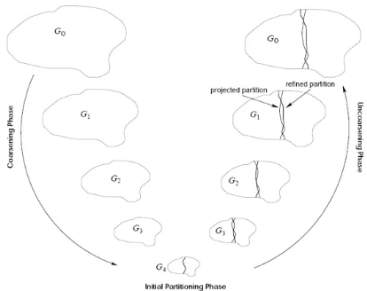
An highly successful strategy for graph partitioning has been the idea of multi-level parti-tioning. The original graph is first coarsened into a sequence of smaller and smaller graphs by collapsing edges and nodes. The smallest graph is then partitioned using slower, pre-cise algorithms. The results of this partitioning are then sequentially applied to the larger graphs and refined, until the results have reached the original graph.
The most successful algorithm that uses this strategy is METIS [57]. The authors introduced improvements at each step of the strategy: edges to be collapsed are chosen using the heavy edge matching strategy, which guarantees a smaller number of levels before reaching a graph small enough to apply partitioning. The partitioning phase is implemented via a simple breadth-first search from a random node, with bias toward nodes that create less cut-edges. Finally, the refinement phase is implemented with a boundary algorithm that greatly improves over the previously used Kernighan-Lin algorithm.
METIS has been quickly expanded to work for hypergraph partitioning [58] and to K-way partitioning [59]. An effort to create a parallelizable version of the program has lead to ParMETIS [60], a version built for multicore machines. The quality of the partitions obtained with this approach does not seem to be of the same quality than the centralized version.
While the quality of METIS is considered very high, there have been improvements on the process by which the graph is coarsened and the different heuristics used at dif-ferent points of the multilevel approach. Lotfifar and Johnson [67] show an improvement in partitioning hypergraphs by filtering ”unimportant edges” using Rough Sets, a data structure useful to extract less important items from a large data set [86].
6.5.5 Streaming partitioning algorithms
CHAPTER 6. PARTITIONING OF LARGE SCALE GRAPHS
Figure 6.5: Illustrative scheme of multilevel partitioning algorithms, from http://masters. donntu.org/2006/fvti/shepel/diss/indexe.htm
streaming scenario.
A more complex example is Fennel [113], an algorithm that computes partitions of only slightly less quality than most centralized algorithms using a fraction of resources. For each incoming vertex, the algorithm computes an objective function that measures the quality of the results for each possible choice. Fennel’s uses a framework to define the objective function, which is shown to contain most of the already known heuristics and can be used to control the complexity of the algorithm.
6.5. APPROACHES TO GRAPH PARTITIONING
already in a partition, the edge will be assigned to that partition. Otherwise, if both nodes are free, the edge will be assigned to the smallest partition. The advantage over Fennel’s approach is that there is no objective function to optimize, therefore the algorithm can be run efficiently even on larger datasets. This heuristic can be run independently on N subsets of the edge set to parallelize the workload, at the cost of lower quality partitions. GraSP [15] shows a real distributed implementation of these greedy strategies. To balance the limited view of each process, the greedy strategy is applied in ns different
passes. At each pass, the requirements for balance become more strict, to allow for higher quality but less balanced partitions at the beginning and then improve the solution toward a more balanced partitioning. The processes only communicate between passes.
HDRF [87] instead concentrates on the greedy rules that are applied on the incoming edges or vertices, with the aim of using the power-law degree distribution of real graphs. If the algorithm needs to create a frontier vertices, it will try to choose the highest-degree nodes.
Another interesting contribution of HDRF is how it can adapt to non-randomly or-dered streams. A particularity of most greedy streaming partitioning algorithms is that, while they perform extremely well in case of randomly ordered streams, they can obtain extremely bad results if the vertices arrive in a specific order, such as one created by a breadth first visit of the graph. Since in many applications the graph is constructed using such processes, the user need to apply a costly random sorting before running the algorithm. HDRF has the advantage of being able to run on partially ordered by correctly setting the parameters of its greedy strategies.
6.5.6 Distributed partitioning
Aside from centralized algorithms that have been expanded to work on parallel and dis-tributed settings, there has been also research on native algorithms for partitioning in distributed and peer-to-peer settings. A few algorithms on distributed graph clustering have also been developed, but they cannot be used for graph partitioning since they do not obtain balanced partitions. Two examples are DIDIC and CDC: DIDIC [41] uses a diffusion process to move information across the graph and make sure that clusters are properly recognized, while CDC [95] simulates a flow of movement across the graph to compute the community around an originator vertex.
ja-be-ja [94] was the first completely decentralized partitioning algorithm based on
CHAPTER 6. PARTITIONING OF LARGE SCALE GRAPHS
size, it will be approved. Since the algorithm has a large risk of falling into a local minima, the authors added a layer based on simulated annealing. At the beginning of the computation, the nodes will be happy to exchange their partitions, even if if this slightly decrease the quality, while toward the end they will be more careful and move partitions only if there is a gain. This peer-to-peer approach is extremely scalable and can therefore be used easily in distributed scenarios.
The authors have also extended their work to apply the same approach to edge par-titioning [93], by changing the peer sampling strategy to allow for exploration of edges instead of vertices.
In Chapter 7 we present an alternative to ja-be-ja, a distributed edge-partitioning
Chapter 7
DFEP: Distributed Funding-based
Edge Partitioning
As presented in Chapter 6, there are many options for graph partitioning that cover the entire spectrum of requirements. There are rough and fast partitioning algorithms for situations in which fast partitioning is more important and algorithms that do more complex computation to get closer to the optimal answer.
The area that has not seen the same level of scrutiny is natively distributed partitioning that can scale to large sizes without losing quality. Here,ja-be-jais the main competitor, but its simulated annealing approach require many iterations to complete. If the users setja-be-ja’s parameters according to the guidelines described by the authors, ja-be-ja
will need several hundred iterations to reach its answer. This large number of iterations may be costly in synchronized settings, where there is a synchronization barrier at the end of each iteration.
In this chapter we presentdfep[45], a novel distributed graph partitioning algorithm
that uses the concept of diffusion and needs only a small coordinator to keep the sizes of each partition as similar as possible. dfep is scalable, computes dense, connected
partitions and can be implemented on top of many vertex-centric programming models.
7.1
Distributed Funding-based Edge Partitioning
The properties that a “good” edge partitioning must possess are the following:
• Balance: partition sizes should be as close as possible to the average size |E|/K, where K is the number of partitions, to have a similar computational load in each partition. Our main goal is to minimize the size of the largest partition.
CHAPTER 7. DFEP: DISTRIBUTED FUNDING-BASED EDGE PARTITIONING
the border of a partition depends on the number of its frontier vertices, the total sum PK
i=1|Fi| must be reduced as much as possible.
There are other, less crucial properties that can cause advantages when specific compu-tation must be done on top of the partitioned graph.
• Connectedness: the subgraphs induced by the partitions should be as connected as possible. This is not a strict requirement and we also illustrate a variant of dfep that relax this condition.
• Path compression: a path between two vertices in G is composed by a sequence of edges. If some information must be passed across this path, it will need to cross partitions every time two consecutive edges belong to different partitions. The smallest the number of partitions to be traversed, the faster the execution will be. Balance is the main goal; it would be simple to just split the edges in K sets of size ≈ |E|/K, but this could have severe implications on communication efficiency and connectedness. The approach proposed here is thus heuristic in nature and provides an approximate solution to the requirements above.
Since the purpose is to compute an edge partitioning as a pre-processing step to help the analysis of very large graphs, we need the edge-partitioning algorithm to be distributed as well. As with most distributed algorithms, we are mostly interested in minimizing the amount of communication steps needed to complete the partitioning.
Ideally a simple solution could work as follows: to compute K partitions, K edges are chosen at random and each partition grows around those edges. Then, all partitions take control of the edges that are neighbors (i.e., they share one vertex) of those already in control and are not taken by other partitions. All partitions will incrementally get larger and larger until all edges have been taken. Unfortunately, this simple approach does not work well in practice, since the starting positions may greatly influence the size of the partitions. A partition that starts from the center of the graph will have more space to expand than a partition that starts from the border and/or very close to another partition.
To overcome this limitation, we introduce dfep (Distributed Funding-based Edge
7.1. DISTRIBUTED FUNDING-BASED EDGE PARTITIONING
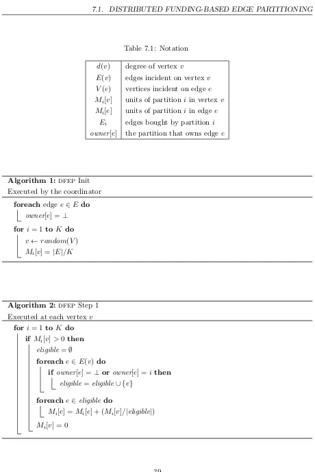
Table 7.1: Notation
d(v) degree of vertexv
E(v) edges incident on vertexv V(e) vertices incident on edge e Mi[v] units of partition iin vertex v
Mi[e] units of partition iin edgee
Ei edges bought by partitioni
owner[e] the partition that owns edge e
Algorithm 1:dfep Init Executed by the coordinator
foreachedge e∈E do owner[e] =⊥
fori= 1 to K do
v←random(V)
Mi[v] =|E|/K
Algorithm 2:dfep Step 1
Executed at each vertexv
fori= 1 to K do if Mi[v]>0then
eligible=∅
foreach e∈E(v) do
if owner[e] =⊥or owner[e] =ithen eligible=eligible∪ {e}
foreach e∈eligibledo
Mi[e] =Mi[e] + (Mi[v]/|eligible|)
CHAPTER 7. DFEP: DISTRIBUTED FUNDING-BASED EDGE PARTITIONING
(a) Step 1 (b) Step 2
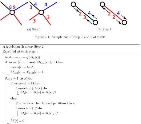
Figure 7.1: Sample run of Step 1 and 2 of dfep Algorithm 3:dfep Step 2
Executed at each edge e best=argmaxp(Mp(e))
if owner[e] =⊥ andMbest(e)≥1then
owner[e] =best
Mbest[e] =Mbest[e]−1
fori= 1 to K do if owner[e] =ithen
foreach v∈N(e) do
Mi[v] =Mi[v] +Mi[e]/2
else
S = vertices that funded partitioniine
foreach v∈S do
Mi[v] =Mi[v] +Mi[e]/|S|
Mi[e] = 0
7.1. DISTRIBUTED FUNDING-BASED EDGE PARTITIONING
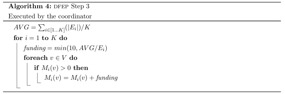
Algorithm 4:dfep Step 3
Executed by the coordinator
AV G=P
i∈[1...K](|Ei|)/K
fori= 1 to K do
funding=min(10, AV G/Ei)
foreachv ∈V do if Mi(v)>0 then
Mi(v) =Mi(v) +funding
the edge and the remaining funding is divided in two equal parts and sent to the vertices composing the edge. In the third step (Algorithm 4), each partition receives an amount of funding inversely proportional to the number of edges it has already bought. This funding is distributed between all the vertices in which the partition has already committed a positive amount of funding.
Figure 7.1a illustrates Step 1 of the algorithm. The vertex has 8 units on the blue partition, 9 units on the red one, two edges are owned by the red partition, one by the blue, and the black one is still unassigned. When Step 1 is concluded, the 9 red units have been committed to the two red edges and the black one, while the 8 blue units have been committed to the blue edge and the black one. The blue partition will be allowed to buy the black edge. Figure 7.1b illustrates Step 2 executed on a single edge. The edge receives 5 red units and 4 blue units, and thus is assigned to the red partition. All the blue units are returned to the sender while the remaining 5−1 red units are divided equally between the two vertices.
dfep creates partitions that are connected subgraphs of the original graph, since
currency cannot traverse an edge that has not been bought by that partition. It can be implemented in a distributed framework: both Step 1 and Step 2 are completely decentralized; Step 3, while centralized, needs an amount of computation that is only linear in the number of partitions.
In our implementation the amount of initial funding is equal to what would be needed to buy an amount of edges equal to the optimal sized partition. A smaller quantity would not decrease the precision of the algorithm, but it would slow it down during the first rounds. The cap on the units of funding to be given to a small partition during each round (10 units in our implementation) avoids the over-funding of a small partition during the first rounds.
CHAPTER 7. DFEP: DISTRIBUTED FUNDING-BASED EDGE PARTITIONING
independently, sends money to the correct edges (that may be on other machines), wait for the other machines to finish Step 1, and executes Step 2. Step 3 must be executed by a coordinator, but the amount of computation is minimal since the current sizes of the partitions can be computed via aggregated counting by the machines. Once the coordinator has computed the amount of funding for each partition, it can send this information to the machines that will apply it independently before Step 1 of the successive iteration. If the coordinator finds that all edges have been assigned, it will terminate the algorithm.
7.1.1 Variants and additions
If the diameter is very large, there is the possibility that a poor starting ver
![Figure 2.1: Structure of the World Wide Web graph, from Graph Structure in the Web [24]](https://thumb-us.123doks.com/thumbv2/123dok_us/537224.2053377/19.595.88.542.127.465/figure-structure-world-wide-web-graph-graph-structure.webp)