Initial Conditions
E
ach stock in a model must be given an initial value. Once this is done, the simulation program will calculate the time history of each model variable for the speci±ed time period. Sometimes initial values for the stocks can be quickly determined, but in other situations this task can be complicated and tedious. This chapter discusses two speci±c di® culties that often arise in specifying initial conditions for the stocks in a model.9.1 Initializing a Model to Equilibrium
Many models are speci±ed for a process that is in equilibrium. That is, the values of the variables in the process are not changing. Often a model is being constructed for the process in order to estimate the impacts of making changes to the structure or operating policies of the process, and in such situations the
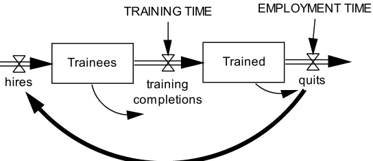
±rst step in the modeling e°ort is to set the model up so that it reproduces the behavior of the existing process. This requires that the model be in equilibrium. Figure 9.1 illustrates a simple model of this type for a personnel process which includes trainees and trained personnel. Trainees require an average of 3 months to train, and they stay in employment for an average of 3 years (36 months) once they are trained. Hiring is done to replace trained employees who quit, and the number of people to hire is determined using an exponential average of the quits over the last 6 months (26 weeks). It is known that there are currently 1000 trained employees, and it is estimated that there are 250 trainees.
When the model is run, the curves shown in Figure 9.1c result. Since it is desired to have the model in equilibrium, clearly something is wrong since the number of trainees and trained personnel both change over time. If the model were in equilibrium, these would remain constant.
114 CHAPTER 9 INITIAL CONDITIONS
EMPLOYMENT TIME TRAINING TIME
hires training quits
completions
Trained Trainees
a. Stock and ow diagram
(01) EMPLOYMENT PERIOD = 36 (02) FINAL TIME = 50
(03) hires = SMOOTH(quits, 26) (04) INITIAL TIME = 0
(05) quits = Trained / EMPLOYMENT PERIOD (06) SAVEPER = TIME STEP
(07) TIME STEP = 0.125
(08) Trained = INTEG (+training completions-quits, 1000) (09) Trainees = INTEG (hires-training completions, 250) (10) training completions = Trainees / TRAINING PERIOD (11) TRAINING PERIOD = 3
b. Vensim equations
CURRENT
Trainees
400
300
200
100
0
0
25
50
Time (Month)
CURRENT
Trained
2,000
1,750
1,500
1,250
1,000
0
25
50
Time (Month)
a. Trainees b. Trained
CURRENT
Trainees
100
95
90
85
80
0
25
50
Time (Month)
CURRENT
Trained
2,000
1,750
1,500
1,250
1,000
0
25
50
Time (Month)
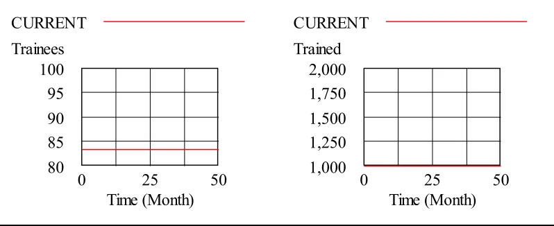
Figure 9.2 Personnel training model (modi ed initial conditions)
the in ows and out ows to \Trainees" to be equal), and \training completions" must be equal to \quits" (for the in ows and out ows to \Trained" to be equal. However, as equations (03) and (10) in Figure 9.1b show, the ow \training completions" is equal to Trainees/TRAINING TIME, and the ow \quits" is equal to Trained/EMPLOYMENT TIME. Therefore, it is not possible to set both of the stocks Trainees and Trained independently. Speci±cally, for the rates \training completion" and \quits" to be equal it must be true that
Trainees
TRAINING TIME =
Trained
EMPLOYMENT TIME
Thus, for the values of Trained, TRAINING TIME, and EMPLOYMENT TIME speci±ed above, it must be true that Trainees = 1;000 (3=36) = 83:3, which is considerable di°erent from the value of 250 that was assumed in the Figure 9.1 model.
Rather than doing all this arithmetic by hand, it may make sense to enter the equation for the initial value of Trainees into the equation for this stock. This requires replacing equation (09) in Figure 9.1b with
(09) Trainees = INTEG (hires-training completions,
Trained * (TRAINING PERIOD / EMPLOYMENT PERIOD))
The results of making this change to the Figure 9.1 model are shown in Figure 9.2. Now the model is in equilibrium.
116 CHAPTER 9 INITIAL CONDITIONS
9.2 Simultaneous Initial Conditions
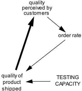
A second type of di® culty that can arise in specifying initial conditions involves the presence of simultaneous equations. Vensim and other similar simulation programs cannot solve simultaneous equations, and therefore it is not possible to set up initial conditions which require solving simultaneous equations. Such simultaneous equations can occur when a causal loop structure in a model in-cludes only auxiliary variables. Figure 9.3 illustrates a model with this di® culty. This is a model where the quality of a product is determined by the testing that is done on the product, and the order rate is impacted by the quality perceived by the customer. When the quality perceived by the customer is equal to one, there is an order rate of 10,000 units per month. In order to provide a product with a quality of one, each unit shipped must receive a testing e°ort equal to one hour of testing. Thus, at a shipping rate of 10,000 units per month, a TESTING CAPACITY of 10,000 hours per month is required. The quality perceived by the customer is an exponential smooth of the actual quality of the product shipped with a smoothing period of 6 months. That is, the customer perception of product quality changes more slowly than the rate at which actual product quality changes.
Everything appears to be correct in this model for it to be initialized to equilibrium. The TESTING CAPACITY is equal to 10,000 hours per month, which is the capacity required to maintain a product quality equal to one, which in turn is the quality required to have an order rate of 10,000 units per month. Hence it appears that the model in equilibrium. However, when you attempt to run the model, Vensim provides the following message: \Model has errors and cannot be simulated. Do you want to correct the errors?" If you click the Yes button, you see a further message that says there are \Simultaneous initial value equations."
The di® culty is that there are simultaneous initial conditions involving the variables \quality perceived by customers," \order rate," and \quality of product shipped." When Vensim attempts to solve for any of these variables, it ends up circling around back to the same variable. We know that the conditions speci±ed in the Figure 9.3b equations are consistent, and they imply an order rate of 10,000 units per month with a quality of one, but Vensim is not able to determine this. The SMOOTHI function is provided by Vensim to handle such situations. This has the same functionality as the SMOOTH function except that it allows you to specify an initial value for the output of the function. (Recall that with the SMOOTH function the initial output value of the function is equal to the initial input value.) The di® culty with simultaneous initial values is resolved by replacing equation (05) in Figure 9.3b with the following:
(5) quality perceived by customers =
SMOOTHI(quality of product shipped, 6, 1)
quality perceived by
customers
quality of product shipped
TESTING CAPACITY
order rate
a. Stock and ow diagram
(1) FINAL TIME = 50 (2) INITIAL TIME = 0
(3) order rate = 10000 * quality perceived by customers (4) quality of product shipped = TESTING CAPACITY /order rate (5) quality perceived by customers
= SMOOTH(quality of product shipped, 6) (6) SAVEPER = TIME STEP
(7) TESTING CAPACITY = 10000 (8) TIME STEP = 0.125
b. Vensim equations