Approximate Explicit MPC and Closed-loop Stability: Analysis based on PWA Lyapunov Functions

PhD Dissertation

International Doctorate School in Information and Communication Technologies

DISI - University of Trento

Approximate Explicit MPC and Closed-loop Stability

Analysis based on PWA Lyapunov Functions

Sergio Trimboli

Advisor:

Prof. Alberto Bemporad

IMT Institute for Advanced Studies Lucca

Abstract

Acknowledgements

This thesis is the result of three years of intense research partially supported by the European Commission through project MOBY-DIC “Model-based synthesis of digital electronic circuits for embedded control” (FP7-INFSO-ICT-248858). I would like to express here the pleasure I had in working together with Prof. Alberto Bemporad. He gave me the possibility to gain a lot of experience in advanced control topics. Alberto, I would like to thank you for sharing your knowledge with me. This thesis, but more important the work possibilities I had, would never happen without your support.

Also, I am grateful to all my co-authors for collaborating in a very productive way. Stefano, Ilya, Matteo, Daniele, Marco, Tomaso, thank you for all the time and knowledge we shared together.

I would particularly like to extend warm thanks to the Committee of this thesis, Marco Storace, Mircea Lazar, Francesco Biral and Thorsten Hestermeyer. Special thanks are for Matteo. Without his guidance and experience, most of this thesis would be never carried out. Matteo, thank you for sharing your methodology and professional abilities. I would also thank you, my friend, for supporting me during my blackout together with Antonio and Laura.

Antonio, your infinite patience and your infinite respect are the abilities that I recognize the most in you. Thank you for all your support, my friend.

valuable friendship during the years in Trento. I would not spend too many words to explain that I found friends in you. I would only say thank you guys. Davide, Simone, Daniele, Emiliano, Alessandro, Sara, Giulio, Ilaria, Rudy, Fabio, Alfio, Stefano thank you for the time we spent together during my first studies in Siena. Thank you for introducing me in the real Ph.D. lifestyle. Finally, I would like to thank my family for the immense support I received in those years (and still now). Antonio and Tina, I am very lucky and I am glad to be your son. This thesis and this Ph.D. is the result of the freedom I had in choosing my way, since of your sacrifices and my effort. I wish to thank Giuliarosa and Walter for their advices and insight. Thank you, with love.

1 Introduction 1

1.1 The problem . . . 3

1.2 Contribution . . . 4

1.3 Summary of publications . . . 5

1.4 Structure of the Thesis . . . 6

1.5 Basic notations and definitions . . . 7

2 State of the Art 9 2.1 Framework . . . 9

2.1.1 MPC algorithm . . . 9

2.1.2 Hybrid models . . . 12

2.1.3 Explicit MPC . . . 13

2.1.4 Switched MPC . . . 15

2.2 Controller circuit implementation . . . 15

2.3 Stability analysis . . . 17

3 Explicit HMPC approximation and FPGA implementation 21 3.1 Circuit implementation of continuous PWAS functions . . . 22

3.2 Generalization to a class of discontinuous functions . . . 24

3.2.1 An example . . . 28

3.3 Switched MPC . . . 30

3.4 Experimental validation . . . 33

3.4.1 Model and control description . . . 34

3.4.2 FPGA implementation . . . 35

4 Closed-loop stability analysis 41 4.1 Problem formulation . . . 42

4.2 Reachability analysis . . . 44

4.2.1 One-step reachability analysis . . . 44

4.2.2 Fake dynamics and extended system . . . 45

4.2.3 Case of additive disturbances only . . . 46

4.3 PWA Lyapunov analysis for the extended system . . . 48

4.3.1 Asymptotic stability . . . 48

4.3.2 Ultimate boundedness . . . 53

4.3.3 Feasibility issues . . . 60

4.4 Invariance analysis . . . 61

4.5 Input-to-State Stability . . . 63

4.6 Simulation examples . . . 66

4.6.1 Uniform asymptotic stability . . . 68

4.6.2 Uniform ultimate boundedness . . . 72

4.6.3 Input-to-state stability . . . 72

5 Conclusion 77

Bibliography 81

3.1 Number of elementary devices to evaluate a discontinuous PWAS 29 3.2 Controllers dimensions . . . 38

2.1 Implicit MPC algorithm . . . 10

3.1 Two-dimensional domain with discontinuities. . . 25

3.2 One-dimensional discontinuous PWAS function . . . 27

3.3 Architecture to implement discontinuous functions . . . 29

3.4 PWA state partitions for u = 25◦C. . . 36

3.5 Differences between manipulated variables of HMPC and SwMPC for r_y = 30. . . 37

3.6 HMPC (blue) vs. PWAS (black). . . 39

4.1 The invariant set _XH for case A is constituted by the union of the regions of the explicit MPC and the box _{XH \ X} (the grey rectangle on the left) . . . 69

4.2 The PWA Lyapunov function for the extended system in case A 70 4.3 The invariant set _P obtained in case A . . . 71

4.4 The PWA Lyapunov-like function for the extended system in case B . . . 73

4.5 The invariant set _P and the terminal set _F (shaded) in case B . . 74

4.6 The sets _{P ≡ X} and _R(_P)_⊕B∞₂ (in black) in case C . . . 76

Introduction

During the last decades Model Predictive Control (MPC) has become the most used technology in highly automated industry [4]. Right now MPC is a stan-dard control approach for both large and medium/small scale processes, even if they are highly complex and multivariable. The word modelin the acronym MPC stands for model-based, while the word predictive means that there is a so-called prediction of the future behavior of the process when selecting the control action.

MPC exploits the knowledge of a dynamical model that describes the plant be-havior in the time domain (usually a state-space model), and is based on an opti-mization problem that minimizes a cost function, usually leading to a quadratic programming problem. Due to physical reasons, the plant actuators are often constrained to operate in a certain range and this implies the imposition of con-straints in the optimization algorithm associated with the MPC control law. It is clear that the constraints on the state, input and output of a dynamical system are embedded in the MPC algorithm and are not imposeda posteriori, as occurs in classical control theory (e.g., PID controllers).

One basic block of MPC strategy is the state-space mathematical model. The

2

interactions between the state variables are described by a set of differential or difference equations, for continuous-time and discrete-time models, respec-tively. In general, the simpler is the model in terms of number of states, the better it is for MPC design.

There exist two main formulations for MPC, the implicit MPC and the explicit MPC. If the system is linear with linear constraints (or can be approximated by such a system), one can map the implicit MPC formulation to an equivalent explicit MPC formulation. By solving an off-line multi-parametric linear or quadratic optimization problem (mpLP, mpQP), the implicit controller can be mapped to a piecewise affine (PWA) explicit control law, that can be evaluated on-line rather easily [1].

The on-line computational complexity of the explicit MPC algorithm can be es-timated exactly. The complexity of the off-line multi-parametric optimization problem grows very quickly with respect to the number of constraints in the MPC problem. As a result, for a very large scale problem, the implicit MPC strategy may be the only viable solution.

Technological innovation drives the attention to a class of models that can deal with continuous and discrete components of systems. The dynamical model exploited in the MPC technology can integrate logical rules, switching physical laws and different kind of operating constraints. As a matter of fact, the hybrid system class of dynamical models integrating logical behavior has been devel-oped [7].

complexity. The closed-loop stability and optimality analysis are only two of the currently open problems in the MPC research community. Many are the milestone papers, for instance [30], in which the researchers undertake the sta-bility and the optimality issues. Also the MPC robustness problem is addressed in [8], in which the authors survey the possible presence of uncertainty in the dy-namical model description together with the stability and performance issues. The aim of this thesis is to develop low complexity solutions for the control problem based on an MPC strategy, even if the model is hybrid, with partic-ular attention to real-time implementation issues. This involves the stability problem, that must be solved. The stability results will provide the theoreti-cal background for low complexity MPC solutions in the hybrid explicit MPC framework.

1.1

The problem

For time-critical applications the implicit MPC solution is not suitable, hence the explicit solution is more compatible. In the explicit MPC strategy, the fea-sible set of the multi-parametric optimization problem is bounded and the dy-namics are continuous function in that set. The assumption of a bounded set is not restrictive when it is coupled with real life applications issues.

1.2. CONTRIBUTION 4

complex multi-parametric optimization problem. The implementation of the re-sulting explicit PWA control law, assuming one is able to determine it offline, in the closed-loop can be very hard, due to the large number of regions (i.e. the lookup table is hard to store and to search).

The main problem is that the explicit MPC solution is employed when the sam-ple time must be small, but for large controller (i.e. too many regions) this leads to an inapplicable solution. As a result of the analysis of the state of the art in the hard real time control framework, the target of this thesis is the study of low complexity solution for explicit MPC of PWA systems (e.g., switching MPC), by also addressing the closed-loop stability problem for this class of systems. Moreover, the synthesized low complexity controller can be circuit implementable, thus leading to a complete bundle that fulfills the requirements on sampling time, circuit architecture, controller performances and closed loop-stability.

Right now, the literature results on explicit MPC stability are not directly appli-cable to low complexity solutions. For instance, if the low complexity controller is the result of a union of several PWA laws (i.e. switching MPC), right now there are few and patchy results giving a stability region in which the controller will be stabilizing for the closed loop, even if the switching MPC can be rep-resented as a PWA control law (i.e. union of PWA). In this case, the stability analysisproblem is addressed in this thesis.

1.2

Contribution

system, we derive an explicit controller in the form of a possibly discontinuous piecewise-affine function. This function is then approximated by resorting to piecewise-affine simplicial functions, which can be implemented on a circuit by extending the representation capabilities of a previously proposed architec-ture to evaluate the control action. The architecarchitec-ture has been implemented on FPGA and validated on a benchmark example related to an air conditioning sys-tem.

Secondarily, this thesis proposes a method to analyze uniform asymptotic sta-bility, uniform ultimate boundedness, and input-to-state stability of uncertain piecewise affine systems whose dynamics are only defined in a bounded and possibly non-invariant set_X of states. The approach relies on introducing fake dynamics outside _X and on synthesizing a piecewise affine and possibly dis-continuous Lyapunov function via linear programming. The existence of such a function proves stability properties of the original system and allows the deter-mination of a region of attraction contained in_X. The procedure is particularly useful in practical applications for analyzing the stability of piecewise affine control systems that are only defined over a bounded subsetX of the state space, and to determine whether for a given set of initial conditions the trajectories of the state vector remain within the domain_X.

1.3

Summary of publications

This thesis is based on the following publications.

1.4. STRUCTURE OF THE THESIS 6

• M. Rubagotti, S. Trimboli, D. Bernardini and A. Bemporad, Stability and invariance analysis of approximate explicit MPC based on PWA Lyapunov functions, in 18th IFAC World Congress, Milano, Italy, 2011.

• T. Poggi, S. Trimboli, A. Bemporad and M. Storace, Explicit hybrid model predictive control: discontinuous piecewise-affine approximation and FPGA implementation, in 18th IFAC World Congress, Milano, Italy, 2011.

1.4

Structure of the Thesis

gathered in Chapter 5.

1.5

Basic notations and definitions

Let _R, _R+, _Z and _Z+ denote the sets of reals, non-negative reals, integers and non-negative integers, respectively. The floor function _b·c of a _{∈ R} is defined as the largestb _{∈ Z} such that a _≥ b. The symbol _{k · k}represent any p-norm of a vector, while_{k · k∞} represents the infinity norm. With respect to the infinity norm, we define the norm ball of radiusχ >0asB∞_{χ ,{}a _{∈ R}n : _ka_{k∞ ≤}χ_}. Given a discrete-time signalv : _{Z+ →R}nv, the sequence of the values ofvfrom the zero instant to the k-th instant is denoted by v_[k]. The norm of a sequence is defined as _kv_{[k]k ,} sup_{kv(i)_k}, for i = 1, ..., k. Given a set _{A ⊆ R}n, its interior is denoted byint(_A), its closure by_A¯, and its convex hull byconv(_A). If _A is a polyhedron, the set of the vertices of _A¯ is denoted by vert( ¯_A). A bounded polyhedron is called polytope. Given two sets _{A ∈ R}n and _{B ∈ R}n, the Minkowski sum is _{A ⊕ B , {}a + b : a _{∈ A}, b _{∈ B}}. A function γ :

R+ → R+ is called K-function if it is continuous, positive definite, and strictly

increasing. A functionφ : _{R+ ×Z+ → R+} is a _KL-function if, for each fixed k _≥ 0, φ(_·, k) is a _K function, for each fixed c _≥ 0, φ(c,_·) is decreasing, and φ(c, k) _→0ast _{→ ∞}.

Consider a generic discrete-time nonlinear system

1.5. BASIC NOTATIONS AND DEFINITIONS 8

Definition 1 (One-step reachable set). Given a set _{X ⊂ R}n and system dynam-ics (1.1), the one step reachable set from _X is

R(_X) _{, {}y _{∈ R}n : y = f(x, v), v _{∈ V}, x _{∈ X }}

Definition 2 (RPI set). A set _{F ⊂ R}n is called robustly positively invariant (RPI) with respect to dynamics (1.1) if, for allx _{∈ F} and allv _{∈ V}, f(x, v) _∈

F.

Definition 3 (Uniform asymptotic stability). Given a set _{X ⊆ R}n with 0 _{∈ X}, system (1.1) is uniformly asymptotically stable in _X (UAS(_X)) if there exists a KL-function φ such that, for all the initial conditions x(0) _{∈ X} and for all the sequences v_[k] with v(i) _{∈ V}, i = 0, ..., k, _kx(k)_{k ≤} φ(_kx(0)_k, k), for all

k _{∈ Z+}.

Definition 4(Uniform ultimate boundedness). Given a set_{X ⊆ R}nand an RPI setF ⊆ X, with0 _∈ int(_F), system(1.1)is uniformly ultimately bounded from

X to _F (UUB(_X,_F)) if, for all a > 0there existT(a) > 0such that, for every x(0) _{∈ X} with _kx(0)_{k ≤} a, x(T) _{∈ F} for all the sequencesv_[k] withv(i) _{∈ V},

i = 0, ..., k.

Definition 5 (Input-to-state stability). Given a setX ⊆ _Rn with 0 _{∈ X}, system (1.1) is input-to-state stable in _X (ISS(_X)) if there exist a _KL-function φ and a _K-functionγ such that, for all the initial conditionsx(0) _{∈ X} and for all the sequencesv_[k]withv(i) _{∈ V},i = 0, ..., k,_kx(k)_{k ≤} φ(_kx(0)_k, k)+γ(_kv_[k−1]k),

State of the Art

2.1

Framework

2.1.1 MPC algorithm

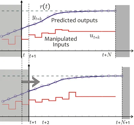
The use of a prediction model, the use of an optimization problem subject to constraints and the receding horizon strategy are the three key principles for stating the MPC algorithm. The control algorithm involves the evaluation of an on-line and open-loop optimization subject to state, input and output con-straints, in which the prediction model is incorporated. Since only the first input of the optimal sequence is applied, the MPC methodology is also called receding horizon.

Referring to Figure 2.1, an instant detailed description of the implicit MPC algo-rithm is given. At each discrete-time t, the measurements y_t acquired from the sensors and the dynamical model are used in order to predict the plant behavior. The state prediction is computed among a N-step time window (N is usually called prediction horizon). The optimal input sequence u∗_t+k is computed by minimizing the related cost function. According to the receding horizon con-trol paradigm, only the first element of the optimal sequenceu∗ is applied as the

2.1. FRAMEWORK 10

min

N

�

−

1

k

=0

�

W

y

(

y

t

+

k

−

r

(

t

))

�

2

+

�

W

∆

u

∆

u

t

+

k

�

2

s.t.

x

t

+

k

+1

=

Ax

t

+

k

+

Bu

t

+

k

y

t

+

k

=

Cx

t

+

k

+

Du

t

+

k

∆u

t

+

k

=

u

t

+

k

−

u

t

+

k

−

1

u

min

≤

u

t

+

k

≤

u

max

∆

u

min

≤

∆

u

t

+

k

≤

∆

u

max

y

min

≤

y

t

+

k

≤

y

max

x

t

=

x

(

t

)

, k

= 0

, . . . , N

−

1

!"#

$%&'#'%()%*+%,-./0123

E5;-21%:4F%2<@0157G.

#

!"#$%&"'((%&")*+",-.)"/()01'%"1/2+"

u

*(

t

)

41-3567-3%087/879

:2;5/8<27-3

=;/879

t t

>#

t

>

N

u

r

3

t

4

t

>#

t

>&

t

>

N

>#

!"

!"#"$%&#

t

'()

"

5+)"$+6"1+'.7-+1+$).

8"-+(+')")*+"/()0109')0/$:";$<"./"/$"="

""""

%*3?2;72@-%0A%1-/-27-3%0;B<5;-%0/75.5C2750;D%

*++,-!./0

y

!"

!"#"$%&

t

)

"./%2+"'$"

12"$%34#516"714

"(-/>%+1"/2+-"'"?7)7-+"*/-09/$"/?

N

.)+(.

@*0."0."'"

893:73"$5#271;73%%$6;#<=>?

(-/>%+1"60)*"-+.(+A)")/")*+".+B7+$A+

/?"0$(7)"0$A-+1+$)."C

u

t

8"=8"C

u

t

+

N

-1

venerdì 7 gennaio 2011

inputu_t+1of the real plant. At the next time step t+ 1, a new optimization prob-lem is solved by exploiting the new measurements, and only the first eprob-lement of the resulting optimal control sequence is applied to the plant. As a result of the receding horizon strategy, it follows that the control action is applied in a closed-loop fashion.

In general the dynamical model can be nonlinear, the cost function can be a2 -norm,1-norm or _∞-norm and the constraints can be time varying. A nonlinear dynamical system implies a more complicated optimization algorithm. For a1 -norm or a _∞-norm cost function is sufficient a linear programming algorithm, while for a2-norm cost function is required a quadratic programming algorithm. Moreover, time varying constraints imply a high computational burden. In the following, a general formulation of MPC problem is stated.

Definition 6(Problem). Let N _≥ 1 be given, let_{X ⊆ R}n and _{U ⊆ R}m be sets which represent the state and the input constraints, respectively, and contain the origin in their interior. The prediction model is x_k+1 = g(x_k, u_k), k _≥ 0, with g : _Rn _{× R}m _{→ R}n a nonlinear, possibly discontinuous function with g(0,0) = 0. Let F : _Rn _{→ R+} with F(0) = 0 and L : _Rn _{× R}m _{→ R+} with L(0,0) = 0be known mappings. For each discrete time instantk _≥0letx_k the measured state, letx_{0|k ,} x_k and minimize the cost function

J(x_k,u_k) _, F(x_N|k) +

N_X−1

i=0

L(x_i|k, u_i|k) (2.1)

over all input sequences u_{k ,} (u_0|k, . . . , u_N−1|k)subject to the constraints x_{i+1|k ,} g(x_i+1|k, u_i|k) , i = 0, . . . , N ₋1, (2.2)

2.1. FRAMEWORK 12

In Problem 6, the functionF denotes the terminal cost, whileL denotes the stage cost and N is the prediction horizon. The termx_i|k denotes the predicted state at future instant i, whilek is the actual instant. The state previewx_i|kis ob-tained by applying the input sequence _{u_{i|k}i=0,...,N−1} to the dynamical model, with the measured state x_k = x_0|k as initial condition. The optimization vari-able in the minimization of the cost function J(x_k,u_k) is the input sequence

{u_{i|k}i=0,...,N−1}. Suppose that the problem of minimizing (6), subject to (2.2), (2.3), (2.4), is feasible and let _{u∗_{i|k}i=0,...,N−1} denote an optimal solution. Ac-cording to the receding horizon strategy, the MPC control action uM P C(x_k) is obtained as the first element of the optimizer u∗ = _{u∗_{i|k}i=0,...,N−1}

uM P C(x_k) _,u∗_0|k, k _≥ 0 (2.5)

2.1.2 Hybrid models

A hybrid system is a system whose behavior is characterized by several modes of operation. For each mode there is a differential or difference equation set describing the continuous time or discrete time dynamics. The switch between the models occurs when a particular event happens. These events can be caused by variables crossing specific thresholds (state event), by the elapsing of certain time periods (time events), or by external inputs (input events) and, for exam-ple, they can be modeled as a finite state machine. Due to switch acting in the hybrid system, the dynamics can be discontinuous. Also, the stability analysis is much harder than in the case of a single operating mode system.

of analysis. The trade-off results in a simpler model representation, but suffi-ciently structured in order to represent a industrially relevant process. Without loss of generality, in this paper the author considers thepiecewise affine(PWA) functions as the class of hybrid models, defined as follows

Definition 7 (PWA Function). A function z(x) : X _{→ R}s, where X _{⊆ R}n is a polyhedral set, is PWA if it is possible to partition X into convex polyhedral regions,CR_i, andz(x) = Hix+ ki, ∀x _∈ CR_i.

In particular, a PWA model is described by the following definition

Definition 8(PWA Model). A PWA dynamical model is the set of discrete time linear systems

x(k + 1) = A_ix(k) +B_iu(k) +f_i y(k) = C_ix(k) +D_iu(k) +g_i

i : H_ix(k) +L_iu(k) _≤K_i, i = 1, . . . , s (2.6) whereA_{i ∈ R}n×n, B_{i ∈ R}n×m, C_{i ∈ R}p×n, D_{i ∈ R}p×m, f_{i ∈ R}n, g_{i ∈ R}p are the state space affine models, i is the active mode at time k and H_i, L_i, K_i are matrices of appropriate dimension.

In the Definition 8, for each i, the polytopic set depends on the state x(k)

and the input u(k) of the system. All the sets are polytopic, hence bounded by definition.

2.1.3 Explicit MPC

al-2.1. FRAMEWORK 14

gorithm is time unpredictable, hence it is not suitable for hard real-time imple-mentation, as it does not provide guarantees on the execution time. There are a lot of processes for which implicit MPC is suitable, for instance a low fre-quency chemical plant, for which the execution time is not really important. A hard real-time control loop must be time predictable, certifiable (i.e. provides guarantee) and relatively fast. However, the effort of the researchers in the field of the optimization algorithms has produced solutions to speed-up the optimiza-tion algorithm, for example the very fast active set strategies [21]. One of the most important result in the hard real-time control is addressed in the explicit solution of the implicit MPC strategy [5].

The idea behind the explicit MPC is to solve off-line several implicit MPC in-stances for all x_k within a given set X = _{x _{∈ R}n : Hx _≤ K_{} ⊂ R}n, and to make the dependence of the input on the state explicit. The set X is assumed to be polytopic (i.e. bounded set and described by linear inequalities). As a result, by solving a multi-parametric program, the equivalent explicit solution of the implicit ones is a piecewise affine function of the state

u(k) =Fix(k) +Gi

if Hix(k) _≤ Ki (2.7)

wherei indexes thei-th region _Rin the explicit linear MPC.

Also, for a hybrid model, under the assumption of bounded state and linear cost function, the explicit MPC solution is a PWA function of the state.

code can run in high speed, the explicit MPC is suitable for time-critical appli-cations.

2.1.4 Switched MPC

The architecture described in the previous sections can be used to implement an explicit SwMPC controller in approximate form. In this section we summarize the main elements of the SwMPC control strategy. A MLD system subject to constraints can be controlled through an implicit HMPC strategy. The explicit HMPC strategy can be applied to a MLD model, after recasting it to an equiv-alent PWA form. A suitable strategy to control (2.6) in state feedback, subject to state and input constraints, is the explicit HMPC [2]. This approach requires enumerating all the feasible switch sequences between the dynamicsiand solv-ing a multi-parametric quadratic problem for each sequence. Storsolv-ing all the control gains leads to a large use of memory blocks in the FPGA implementa-tion with respect to a simpler controller such as the SwMPC. Considering only the sequences for which the region i is the same during the prediction steps, since the constraints that define the PWA regions are ignored after the first pre-diction step, the number of multi-parametric quadratic problems to be solved is equal to the number of PWA regions, leading to a suboptimal solution to the control problem. A formal definition of the SwMPC will be given in Sec. 3.3.

2.2

Controller circuit implementation

2.2. CONTROLLER CIRCUIT IMPLEMENTATION 16

generation strategy was developed in [36]. Starting from a model, through the definition of a model-based control strategy suitable for the implementation in an embedded architecture, the problem of implementing the control strategy was also investigated for parallel architectures in [28]. Often a system that inte-grates continuous dynamics and logical structures can be described as a mixed-logic dynamical system (MLD). A suitable strategy to control a MLD system subject to constraints is hybrid model predictive control (HMPC). In order to obtain a HMPC, one has to solve on-line a integer quadratic or a mixed-integer linear programming problem. For a high-dimensional model, solving this kind of problems may be computationally too expensive for fast real-time application [14].

Explicit reformulations of HMPC can be carried out by solving off-line a sequence of multi-parametric quadratic or linear problems [14]. The result-ing solution is a possibly discontinuous piecewise affine (PWA) function of the state. In other words, the control modes are linear affine over polytopes partitioning the state domain, thus making this approach more suitable for the embedded control implementations. Storing the gains of the explicit HMPC re-quires larger and larger memory blocks in the electronic implementation as the number of partitions grows. Moreover, in order to evaluate the control action, the pre-computed gains should be selected, according to the state value, from a look-up table associated to the explicit controller. As a result, since the gains selection from the look-up table can be made by a binary-tree search [41], or by other more sophisticated algorithms, determining the correct mode can be a hard problem if the number of regions is too large.

instance in [18], where a PWA system is controlled by a set of linear MPC controllers, each one defined over a different polytope of the domain. In explicit form, SwMPC is basically a set of patched PWA controllers. For each i-th region_Ri of the domain, a linear MPC problem is solved, whose solution is a continuous PWA function defined over a polytopic partition of the region. Note that a MLD model can be converted in an equivalent PWA formulation [2].

The resulting PWA control function may be discontinuous only at the bound-aries of the regions. The overall number of polytopes obtained with the ex-plicit SwMPC approach is typically much lower than the one obtained with the explicit HMPC, especially when the number of optimization variables grows. However, the SwMPC complexity reduction with respect to HMPC is not cost-less, since optimal switching sequences are restricted to constant mode se-quences, possibly breakinga-priori stability properties. However, a-posteriori stability analysis of the SwMPC can be performed exploiting the results in [20] and in [38].

2.3

Stability analysis

In the last decade the interest in studying the dynamical properties of piece-wise affine (PWA) systems has increased considerably, due to their powerful modeling capabilities. Discrete-time PWA models are a special class of hybrid systems that can represent combinations of finite automata and linear dynam-ics, are a good approximation of nonlinear systems [39], and are equivalent to hybrid systems in mixed logical dynamical form [2, 7].

2.3. STABILITY ANALYSIS 18

of a given closed-loop system [6, 17]. In particular, stability analysis becomes fundamental when a PWA control law is synthesized without a-priori guaran-tees of closed-loop stability, for example when explicit model predictive control (MPC) laws [9] are approximated in order to reduce their complexity [1].

The most widely used methods for stability analysis of discrete-time PWA systems are based on piecewise quadratic (PWQ) Lyapunov functions [20]. Such methods rely on the solution of a semi-definite program to get a stabil-ity certificate. As highlighted in [22], the search for a PWQ Lyapunov function can be overly conservative, even with the use of the so-called S-procedure (see e.g. [15]). A valid alternative are PWA Lyapunov functions, that are computed by solving a linear program (LP) [11]. Other types of Lyapunov functions can be used for the same purpose, such as piecewise polynomial Lyapunov func-tions [34]. For an overview of such methods, the interested reader is referred to [11].

Most of the existing literature on stability analysis of PWA systems assumes that the set _X of states in which the PWA dynamics are defined is invariant, as the notion of stability has no practical relevance if the state trajectory exits the domain of definition of the dynamics [11]. However, often the PWA system to be analyzed is defined in a set_X that may not be invariant. A possible approach is to perform a reachability analysis to find the maximum positively invariant set to establish, using a recursive procedure, an invariant subset of the given set

X (see [35], [12, Chap. 4-5] and the references therein). Unfortunately this procedure often leads to very involved solutions, due to the exponential com-plexity of reachability analysis of PWA systems, and in many cases searching the maximum invariant set is an undecidable problem.

Explicit HMPC approximation and FPGA

implementation

In this thesis we extend to discontinuous PWA functions the results of [32, 40], related to the circuit implementation of continuous PWA functions. Recalling Sec. 2.2, where the state of the art regarding the implementation of possibly discontinuous PWA functions in approximate form on fast digital circuits, we restrict our attention to PWA control functions for which each mode is defined over a hyper-rectangular region. This limits the approach to hybrid dynamical systems where threshold conditions only depend on single components of the state vector.

In order to circuit implement the SwMPC solution in an approximate but fast way, we resort to a modified version of the method proposed in [10]. Ac-cordingly, each explicit solution (valid over the i-th hyper-rectangular region) is first approximated by using a PWA continuous function, defined over a reg-ular simplicial partition of the i-th region (called PWAS function). Then, the obtained approximations can be merged into one PWAS discontinuous func-tion, which can be directly mapped on programmable hardware such as a field

3.1. CIRCUIT IMPLEMENTATION OF CONTINUOUS PWAS FUNCTIONS 22

programmable gate array (FPGA).

The architectures able to implement PWAS functions proposed so far in [19, 37,40] perform a linear interpolation of the values of the function at the vertices of the simplex the input belongs to. The main limit of such an approach is that the implementable functions are continuous. If functions with discontinuities that are not perpendicular to an axis were to be implemented, more complex and power-hungry architectures would be necessary [23, 31].

3.1

Circuit implementation of continuous PWAS functions

ofN α-basis functions

f_{P W AS}(z) =

N−1

X

k=0

c_kα_k(z). (3.1)

Once the scaled simplicial domain is defined, the basis functions (belonging to theα-basis) are directly defined as well. Thek-thα-function is PWAS, holds the value 1 at the vertex corresponding to v_k and the value 0 at all the other vertices.

The shape of a given PWAS function f_{P W AS} is coded by the N coefficients c_k in Eq. (3.1), which are the values off_{P W AS} at the vertices v_k of its simplicial partitions. Henceforth, we assume that the coefficients are already determined by a function approximation procedure (see, e.g. [10]).

The coefficients c_k (k = 1, . . . , N) are stored by assigning a proper memory address to each vertex v_k of the simplicial partition. Define β_p : _Nn _{→ Nb}

as the binarizing operator that, given a column vector of n integer values and a precision p, returns a np-long string of bits, concatenating the binary values of the elements of the vector. For instance, if v_k = [2, 0, 5]T and p = 3, then β_p(v_k) = 010 000 101. Then, β_p(v_k) is an unambiguous address for the vertex v_k. The value of f_{P W AS}(z) can be calculated as a linear interpolation of thef_{P W AS} values at the vertices of the simplex containing z, i.e., as a linear interpolation of a subset ofn+ 1coefficientsc_k:

f_{P W AS}(z) =

n

X

j=0

µ_jc_Ωj (3.2)

where theµ_j’s are the weights that givezas a convex combination of the vertices of the simplex that contains it (i.e., z = Pn_j=0µ_jv_Ωj, with Pn_j=0µ_j = 1) and

3.2. GENERALIZATION TO A CLASS OF DISCONTINUOUS FUNCTIONS 24

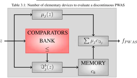
indexkof one of the vertices surroundingz [32]. Ω_j, as well as the interpolation weightsµ_j, depends onz. This dependence is omitted here for ease of notation. As a consequence, the circuit realization of a PWAS function proposed in [40] requires three functional elements:

1. a memory where the N c_k coefficients are stored;

2. a block that finds, for any given inputz, the indicesΩ_j and the coefficients µ_j;

3. a block performing the weighted sum (3.2).

Since the_{ck}’s are stored in a memory,Ωj corresponds uniquely to the address

Ωb_j of thej-th coefficient in Eq. (3.2), through the binarizing operatorβ_p

Ωb_j = β_p(_bz_c+a_j), j = 0, . . . , n (3.3) wherea_j’s are vectors whose components are calculated from the decimal parts of the input z [32].

3.2

Generalization to a class of discontinuous functions

The algorithm presented in Sec. 3.1 can be generalized to include a particular class of discontinuous functions, namely the functions composed of continuous PWAS functions separated by discontinuities that lie perpendicular to a coordi-nate axis. In this case, we can define an index labeling the subregion a continu-ous PWAS function is defined over and use this index to solve the point location problem, i.e. to address correctly the memory containing the coefficients.

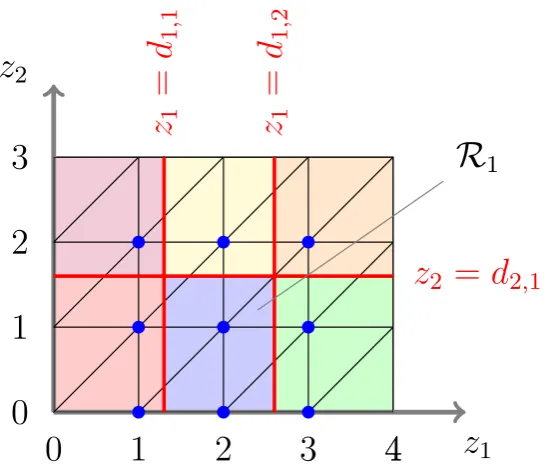
in the formz_h = d_h,t (h = 1, . . . , n; t = 1, . . . , D_h; d_h,t constant) that further partition the domain S into P = Qn_h=1(D_h+ 1) hyper-rectangular regions _Ri (discontinuity partition,i = 1, . . . , P). Figure 3.1 shows an example of a two-dimensional domain of a discontinuous function withm₁ = 4, m₂ = 3,D₁ = 2

and D₂ = 1. Both the regular simplicial partition and the six regions _Ri are highlighted.

z

z

0

0

1

1

2

2

3

3

4

z

=

d

1

z

=

d

2

z

=

d

4

R

Figure 3.1: Two-dimensional domain with discontinuities.

The discontinuous functionf_{P W AS} can be defined as follows:

f_{P W AS}(z) = f_{P W AS i}(z) =

N_X−1

k=0

ci_kα_k(z), _∀z _{∈ Ri} (3.4)

3.2. GENERALIZATION TO A CLASS OF DISCONTINUOUS FUNCTIONS 26

functions (see Eqs. (3.1) and (3.4)). The shape of a particular function f_{P W AS i} is coded by the coefficients related to the vertices that lie inside_Ri and immedi-ately outside of the boundary of _Ri. Thus, most of the coefficients ci_k related to vertices that fall outside_Ri can be discarded. Indeed, we need to consider only the set V_i of the vertices that lie inside the smallest hyper-rectangle containing

Ri defined over the vertices of the simplicial partition. For instance, in Fig. 3.1 the vertices V₁ that define the shape of f_{P W AS1} over _R1 are marked by blue

dots. They are all contained inside the rectangle [1, 3]_×[0, 2]. 1 Then,f_{P W AS i} is completely characterized by the coefficients corresponding to V_i:

f_{P W AS i}(z) = X

k_∈Ki

ci_kα_k(z), z _{∈ Ri},

where_Ki = _{k : v_{k ∈} V_i}.

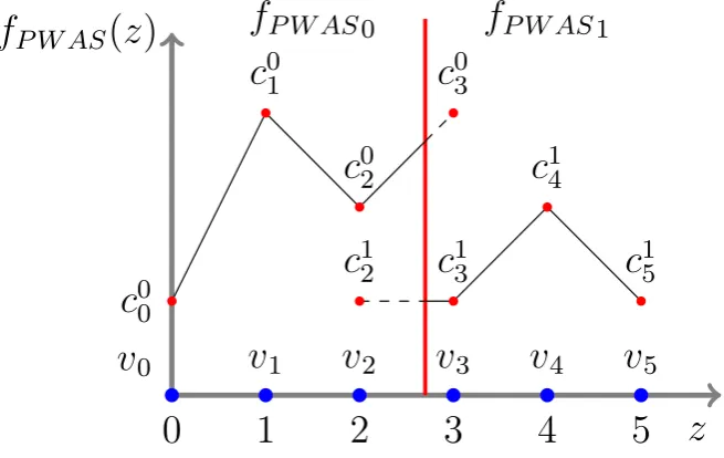
An example of discontinuous PWAS function is shown in Fig. 3.2. In this case, f_{P W AS} is defined over a one-dimensional domain S = [1,5], with one discontinuity (z = d_1,1 = 2.7) and

f_{P W AS}(z) =

  

f_{P W AS0}(z), z _{∈ R0} = [1,2.7)

f_{P W AS1}(z), z _{∈ R1} = [2.7,5]

To calculate f_{P W AS0}, it is necessary to know the value of its coefficients at the vertices v₀, v₁, v₂ (all _{∈ R}0) and v3(∈ R/ 0), then V0 = {v0, v1, v2, v3} and

K0 = {0,1,2,3}. On the other hand, the set of vertices needed to evaluate

f_{P W AS1} is v₃, v₄, v₅ (all _{∈ R1}) and v₂(_{∈ R}/ ₁), then V₁ = _{v₂, v₃, v₄, v_5} and

1_{A formal definition ofViis}

Vh=

(

vk _∈V :vi_∈ argmin

R(vk)⊇Ri

{|R(vk)_|}

)

K1 = {2,3,4,5}. We notice that the correspondence between vertices of the

simplicial partition and coefficients is no longer one-to-one, as both c0₂ and c1₂ are related tov₂ and bothc0₃ andc1₃ are related tov₃.

z

f

(

z

)

0

v

1

v

2

v

3

v

4

v

5

v

f

f

c

c

c

c

c

c

c

c

Figure 3.2: One-dimensional discontinuous PWAS function

Since some coefficients ci_k of each function f_{P W AS i} are in a relation many-to-one with the vertices of the simplicial partition and since they are stored in the same memory, we need to refine the way they are addressed. For any given z = [z₁, z₂, . . . , z_n]T _{∈ Ri}, we can define

r(z) =

     

PD1

t=1u(z1 −d1,t)

PD2

t=1u(z2 −d2,t)

...

PD1

t=nu(zn−dn,t)

      (3.5)

3.2. GENERALIZATION TO A CLASS OF DISCONTINUOUS FUNCTIONS 28

Given a point z, we need to find the rectangle _Ri such that z _{∈ Ri} and the related set of coefficients ci_k. Thus, the index map Ω_j is redefined so that it corresponds uniquely (for any z) to the memory address

Ωb_j = β_p+1(2r(z) +_bz_c+a_j), j = 0, . . . , n (3.6) Finally, a discontinuous PWAS function can be evaluated using the method provided in Sec. 3.1 by substituting Eq. (3.3) with Eq. (3.6). The binary vector β_p−1(r(z)) can be easily obtained by using comparators to process the input z and find the region it belongs to.

To evaluate each function f_{P W AS i} it is possible to use the architecture A proposed in [40], that provides a correct output every p + q + n + 5 clock cycles, where p and q are the number of bits used to code the integer part and the decimal part, respectively, and n is the input dimension. As stated before, the coefficientsci_k defining the shape of f_{P W AS} are stored in a memory and they can be addressed by calculating the strings Ωb_j. Then, we need to modify the way the address is calculated in [40], according to Eq. (3.6). Equation (3.5) is evaluated asynchronously with respect to the system clock through comparators and 1-bit adders when the input vectorz is fed into the circuit.

The number of elementary devices (comparators, adders, multipliers, etc.) required to evaluate a discontinuous PWAS function is reported in Tab. 3.1. The items of the part added to evaluate discontinuous functions are kept separated and described in italic text.

3.2.1 An example

Item Bits #Devices

Comparator q n

Multiplexer n n

ROM 2np_×b 1

Adder/Subtractor n+ 1 n

Adder/Subtractor q n

Multiplier b_×q 1 Comparator p+q Pn_i=1Di

Adder 1 n

Adder p+ 1 n

Shift Register p 1

Table 3.1: Number of elementary devices to evaluate a discontinuous PWAS

µ

(

z

)

=

(

z

)

MEMORY

c

P

µ

c

z

f

COMPARATORS

BANK

≤

Figure 3.3: Architecture to implement discontinuous functions

discontinuities ind_1,1 = 2.1, d_1,2 = 8.5, d_2,1 = 0.9 and d_3,1 = 9.7. We need to retrieve from the memoryn+ 1 = 4coefficientsch_Ω

3.3. SWITCHED MPC 30

a_j depend on the decimal part ofz and assume the values (the reader is referred to [32] for details):

a₀ =

   0 0 0  

, a₁ =

   1 0 0  

, a₂ =

   1 0 1  

, a₃ =

   1 1 1   

By applying Eq. (3.5) we obtain

r(z) =

  

u(z_{1 −}d_1,1) +u(z_{1 −}d_1,2)

u(z_{2 −}d_2,1)

u(z_{3 −}d_3,1)

   =   

1 + 0

1

0

  

Fixing p = 4, the first address is given by

Ωb₀ = β_p+1(2r(z) +_bz_c+a₀)

= β₅([2, 2, 0]T + [2, 4, 1]T + [0, 0, 0]T) = β₅([4, 6, 1]T)

= [00100 00110 00001]

and the others take the values

Ωb₁ = [00101 00110 00001],

Ωb₂ = [00101 00110 00010],

Ωb₃ = [00101 00111 00010].

3.3

Switched MPC

MLD system subject to constraints can be controlled through an implicit HMPC strategy. The explicit HMPC strategy can be applied to a MLD model, after recasting it to an equivalent PWA form. A time-invariant PWA discrete-time model is defined as follows

x(k+ 1) = A_ix(k) +B_iu(k) +f_i (3.7) i : H_ix(k) _≤K_i , i _{∈ I} (3.8) wherex _{∈ R}n×1, u _{∈ R}m×1, A_{i ∈ R}n×n, B_{i ∈ R}n×m, f_{i ∈ R}n×1 characterizes the i-th mode, H_i, K_i are matrices of suitable dimensions defining the i-th re-gion _Ri, _I = _{1, . . . , P_} and P is the number of regions. A suitable strategy to control (3.7), (3.8) in state feedback, subject to state and input constraints, is the explicit HMPC [2]. This approach requires enumerating all the feasi-ble switch sequences between the dynamics i and solving a multi-parametric quadratic problem for each sequence. Storing all the control gains leads to a large use of memory blocks in the FPGA implementation with respect to a sim-pler controller such as the SwMPC. Considering only the sequences for which the region i is the same during the prediction steps, since the constraints that define the PWA regions are ignored after the first prediction step, the number of multi-parametric quadratic problems to be solved is equal to the number of PWA regions, leading to a suboptimal solution to the control problem.

In order to formulate (3.7), (3.8) as standard linear system, fixing the mode i, we merge the affine term f_i in the input matrix B_i. The resulting set of linear systems is a suitable formulation for a set of linear MPCs. Let v(k) be a measured input disturbance such that v(k) = 1,_∀k _≥ 0, then (3.7) can be rewritten as follows

3.3. SWITCHED MPC 32

or, in a more compact way,

x(k+ 1) = A_ix(k) + ¯B_iu¯(k) (3.10) where B¯_i = [Bi fi] and u¯ = [u0_{(k) v(k)]}0_{. Exploiting model (3.10), (3.8) we}

define a set of linear MPCs based on the following quadratic problem:

min

U=[u0, ..., uM]

J(x, U) =

M_X−1

k=0

x(k)0Qx(k)+

+u0(k)Ru(k) +ρ2 s.t. x_min−≤x(k) _≤ x_max+,

u_{min ≤}u(k) _≤ u_max,

x(k + 1) =A_ix(k) + ¯B_iu¯(k) (3.11) whereM is the prediction horizon; the quantitiesx_min, x_max,u_min, u_max are state and input bounds, respectively; is a slack variable, weighted by ρ; R, Q are weight matrices of suitable dimensions; A_i, B_i are the i-th model matrices. At time k, only the first component u₀ of the optimal sequence is applied, in a receding horizon fashion. A SwMPC is a set of linear MPCs based on (3.11) each one defined over its corresponding region _Xi. For each control step, one has to evaluate the active modei and compute the i-th control action.

Problem (3.11) is stated as a regulation of the states to the origin. A reference tracking problem can be recast as partial state regulation problem by extending the state vector and exploiting the same formulation, as follows. Let y(k) =

Cx(k) be the output of model (3.10), (3.8), where C _{∈ R}o×n is the output matrix, then consider the extended state vector x_e = [x0 _r0

identity matrix of ordero. This leads to a reference tracking problem with cost functionJ(x, U) = PM_k=0−1(Cx(k)₋r_y)0Q_y(Cx(k)₋r_y) +u0(k)Ru(k) +ρ2. Exploiting the results in [9], each linear MPC of the SwMPC formulation could be explicitly solved through a multi-parametric quadratic problem, lead-ing to a set of linear explicit MPCs. Moreover, in each region the explicit con-troller is a continuous PWA function of the state. The overall explicit SwMPC controller is defined as follows.

u(k) =F_jix(k) +Gi_j (3.12) if H_jix(k) _≤ K_ji (3.13) wherej indexes the polytopes of thei-th region _Ri in the explicit linear MPC. In the framework described in the previous sections, these polytopes reduce to identical simplexes and the regions are hyper-rectangles.

In the next section, a benchmark for the SwMPC implemented with PWAS in a FPGA reveals the capabilities of the proposed approach, suggesting that the SwMPC performances can get very close to the HMPC ones, at least for functions belonging to the class described in Sec. 3.2.

3.4

Experimental validation

3.4. EXPERIMENTAL VALIDATION 34

function defining the controller is approximated by a PWAS function. We ob-tain a discontinuous PWAS controller, which is implemented on a FPGA by using the architecture introduced in Sec. 3.2.

3.4.1 Model and control description

The state vectorxrepresents two different temperatures, while the inputuis the ambient temperature to be regulated:

x(k) _, hT1(k)

T2(k)

i

, u _,T_amb

The auxiliary variables associated with threshold eventsu_hot, u_cold are such that IF x_{1 ≤} T_c1 OR (x_{2 ≤} T_c2 ANDx₁ < T_h1)

THENu_hot = U_h ,ELSE u_hot = 0

IF x_{1 ≤} T_h1 OR (x_{2 ≤} T_h2 ANDx₁ < T_c1)

THEN u_cold = U_c ,ELSE u_cold = 0 (3.14) whereT_{{c1,c2,h1,h2}} are constant temperatures,U_c represents the air conditioning power flow, U_hrepresents the heater flow.

The hybrid model is stated as follows.

x₁(k+ 1) = x₁(k) +T_s[₋α₁(x₁(k)₋u(k))+ +K1(uhot(k)−ucold(k))] x₂(k+ 1) = x₂(k) +T_s[₋α₂(x₂(k)₋u(k))+

The state and input constraints for the hybrid model are the following.

−10 _≤u(k) _≤ 50

−10 _≤x(k) _≤ 50 (3.16) By exploiting the results of [2], the hybrid model (3.14),(3.15) is translated into an equivalent PWA model, which is defined over a three-dimensional do-main (n = 3, with 2state dimensions and1input dimension) partitioned into 5

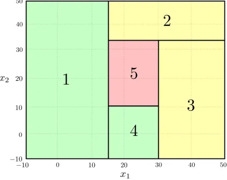
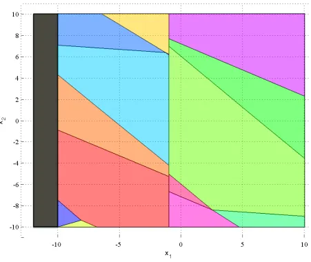
polyhedral regions. As shown in Fig. 3.4, where a section of the PWA model forT_amb = 25◦C is shown, the polyhedral partition has boundaries parallel with respect to the state axesT₁ andT₂. Since the open-loop dynamics in regions 2,

3and in 1, 4 are the same, the MPC calculated over the partition _P associated to region 2 is equivalent to the one calculated in region 3, as well as region 1

shares the same MPC with region4, although on different sets of states.

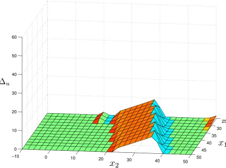
As described in Sec. 3.3, the affine terms in the PWA formulation are con-sidered as constant measured input disturbances in the SwMPC formulation. The target of the controller is to track a referencer_y for y = x₂, while enforc-ing the constraint x_{1 ≥} 25 in addition to the constraints in (3.14), (3.16). The controllers (HMPC and SwMPC) share the same tuning parameters: M = 4, Q_y = 1, R = 0, ρ = +_∞ (corresponding to hard constraints). For a constant reference tracking r_y = 30, Figure 3.5 shows that the difference ∆_u between the manipulated variables in HMPC and SwMPC is negligible in most of the considered points. The controllers characteristics are summarized in Table 3.2.

3.4.2 FPGA implementation

3.4. EXPERIMENTAL VALIDATION 36

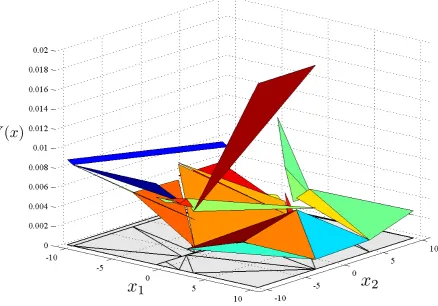
The first step towards the FPGA implementation is the PWAS approximation of each explicit linear MPC by applying the method proposed in [10]. The result of the approximations are five continuous PWAS functions defined all over the domain, partitioned into simplices using m_h = 7 divisions along each dimensional component.

The second step is to merge the five continuous PWAS functions into one discontinuous PWAS functionf_{P W AS}. Since there are two discontinuities along

x

−10 0 10 20 30 40 50

−10

0

10 20

30 40 50

5

2

3

1

4

x

mercoledì 13 ottobre 2010

25 30 35 40 45 50

−10 ₀

10 20 ₃₀

40 50 0

10 20 30 40 50 60

x

x

∆

Thursday, October 14, 2010

3.4. EXPERIMENTAL VALIDATION 38

Item HMPC SwMPC

(for each controller)

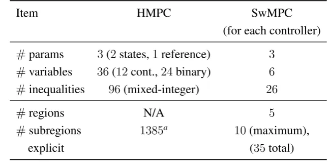
#params 3(2states,1reference) 3 #variables 36(12cont.,24binary) 6 #inequalities 96(mixed-integer) 26

#regions N/A 5

#subregions 1385a _10(maximum),

explicit (35total)

a_{Possible overlapping regions that are never optimal are not removed}

Table 3.2: Controllers dimensions

the first and the second dimensions, the discontinuity partition is composed by nine hyper-rectangular subregions _Ri, i = 1, . . . ,9.

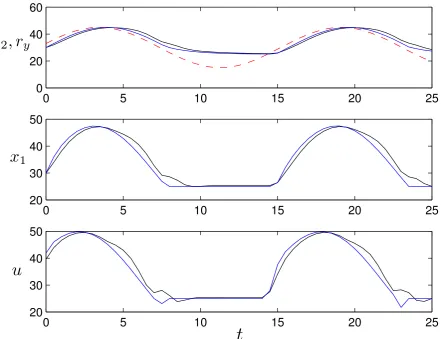
Fig. 3.6 shows the input and state signals obtained using the PWAS approx-imated control and the HMPC approach, where a sinusoidal reference r_y for x₂ is imposed.

Function f_{P W AS} is implemented by resorting to the proposed architecture. To implement the circuit architecture on FPGA we have used a fully generic VHDL description, so that it is possible to change any parameter before pro-gramming the FPGA without editing the VHDL code; these parameters are the input dimension n, the number of bits used to code the integer part (p) and dec-imal part (q) of the input and the number of bits (b) used to code the coefficients ci_k. The position of the discontinuities d_h,t inside the domain and the value of the coefficients ci_k is set through a Matlab routine that allows the configuration of the whole VHDL code.

0 5 10 15 20 25 0

20 40 60

x 2

, r

0 5 10 15 20 25

20 30 40 50

x 1

0 5 10 15 20 25

20 30 40 50

u

t

t

x

u

x

, r

Thursday, October 14, 2010

3.4. EXPERIMENTAL VALIDATION 40

Closed-loop stability analysis

The contribution of this Chapter is the definition of a stability analysis frame-work for discrete-time PWA systems subject to both parametric uncertainties and additive disturbances which are unknown but bounded and defined in poly-topic sets. The proposed method is based on the use of PWA Lyapunov func-tions synthesized via linear programming, and permits to determine if the state converges to the origin (or to a terminal set including the origin). The system dynamics are defined only in a closed polytopic region _X, which is not neces-sarily required to be invariant. By artificially extending the systems dynamics outside _X, the proposed method can determine an invariant subset of _X, in which the dynamics of the original PWA system of interest are defined. The attractiveness of the origin (or that of the terminal set) is determined with re-spect to such a region of attraction. Finally, discontinuities on the boundaries of the partitions are tackled for both the system dynamics and the PWA Lya-punov function, in order to broaden the range of applicability of the proposed approach and to reduce the conservativeness due to the imposition of continu-ity. The presence of discontinuities, however, requires additional attention on technical conditions [26].

4.1. PROBLEM FORMULATION 42

Preliminary results of this thesis focusing only on the asymptotic stability analysis of systems without disturbances or with parametric disturbances are reported in [38] and in [42], respectively.

4.1

Problem formulation

Consider the autonomous discrete-time uncertain PWA system

x(k + 1) = A_i(w(k))x(k) +a_i(w(k)) +E_i(w(k))d(k) ifx(k) _{∈ Xi} (4.1) wherex(k) _{∈ R}n, w(k) _{∈ W ⊂ R}q, d(k) _{∈ D ⊂ R}p,

A_i(w) _, A_i,0 +

q

X

r=1

A_i,rw_r (4.2a)

a_i(w) _, a_i,0 +

q

X

r=1

a_i,rw_r (4.2b)

Ei(w) , Ei,0 +

q

X

r=1

Ei,rwr (4.2c)

W ,

(

w _{∈ R}q :

q

X

r=1

w_r = 1, w_{r ≥} 0

)

(4.2d)

D , nd _{∈ R}p : ˜Hd _≤ ˜ho (4.2e) A_{i,r ∈ R}n×n, a_{i,r ∈ R}n, E_{i,r ∈ R}n×p, with r = 0, ..., q, and k _{∈ Z+},

˜

H _{∈ R}p×η, and ˜h _{∈ R}η. Denote by d₁, . . . , d_{η ∈ R}p the vertices of _D,

D = conv(d₁, . . . , d_η). The sets _Xi, i _{∈ I , {}1, ..., s_}, are (possibly non-closed) polytopes such thatint(_Xi) ₆= _∅, _Xi∩ Xj = ∅,∀i, j ∈ I withi 6= j, and such that _{X ,} Ss_i=1Xi is a closed polytope. The subset of indices _I0 is defined as _{I0 ,{}i _{∈ I} : 0 _{∈ X}¯_i}. The interior of each partition_Xi is defined as

where H_i and h_i are a constant matrix and a constant vector, respectively, of suitable dimensions, and let_X¯_i the closure of_Xi, _X¯_{i , {}x : H_ix _≤ h_i}, i _{∈ I}.

Denote by

x(k+ 1) = A_i,0x(k) +a_i,0 ifx(k) _{∈ Xi} (4.4)

the nominal model of (4.1). Note that dynamics (4.1) may not be continuous with respect to x on the boundaries of the partitions _Xi, while it is continuous with respect tow andd.

Assumption 1. There exists an indexi _{∈ I} such that0 _∈ vert( ¯_Xi),0 _∈ int(_X).

Note that Assumption 1 can be always satisfied. In fact, if the origin is not on a vertex of any polyhedron _Xi, it is always possible to further partition _X to obtain a new set of partitions_Xi which fulfills Assumption 1. Note also that the state trajectories may not be persistent in time, since_X is not necessarily an RPI set, and the dynamics are not defined outside_X.

4.2. REACHABILITY ANALYSIS 44

4.2

Reachability analysis

4.2.1 One-step reachability analysis

Since the set _X is not assumed to be RPI with respect to dynamics (4.1), we must take into account that the trajectories may possibly leave_X, and be there-fore defined only on a finite time interval [0, k_max]. Define the one-step reach-able set from _X

R(_X) _,{A_i(w)x+a_i(w) +E_i(w)d :w _{∈ W}, d _{∈ D}, x _{∈ Xi}, i _{∈ I}} and let

R∪(X) , R(X)∪ X (4.5)

The set _R(_X) can be computed as the union of the one-step reachable sets from all the _Xi, defined as

R(_Xi) _,{A_i(w)x+a_i(w) +E_i(w)d, w _{∈ W}, d _{∈ D}, x _{∈ Xi}}

Note that _R(_Xi) is not a convex set in general. Note that the terms in (4.2a) and (4.2b) can be equivalently expressed as

A_i(w) =

q

X

r=1

(A_i,0 +A_i,r)w_{r ,} q

X

r=1

˜

A_i,rw_r

a_i(w) =

q

X

r=1

(a_i,0 +a_i,r)w_{r ,} q

X

r=1

˜

a_i,rw_r

E_i(w) =

q

X

r=1

(E_i,0 +E_i,r)w_{r ,} q

X

r=1

˜

By relying on the results in [12, Chap. 6], we can compute the convex hulls of the sets_R( ¯_Xi)as

conv _R( ¯_Xi)=

conv

˜

A_i,rv_i,h + ˜a_i,r + ˜E_i,rd_i,µ, r = 1, ..., q, µ = 1, ..., η, h= 1, ..., m_i

wherev_i,h represents each of them_i vertices of_X¯i.

Therefore, an over-approximation of _R∪(_X) in (4.5) is

˜

R∪(X) ,

s

[

i=1

conv _R( ¯_Xi) _{∪ X ⊇ R∪}(_X) (4.6)

4.2.2 Fake dynamics and extended system

As dynamics (4.1) is not defined outside _X, the proposed strategy consists in defining a “fake” dynamics on_R˜_∪(_X)_{\ X}. Let_{XH ⊇ R}˜_∪(_X)be the bounding box of_R˜_∪(_X), i.e., the smallest closed hyper-rectangle containing_R˜_∪(_X), and consider the dynamics

x(k + 1) = ρx(k), ifx(k) _{∈ XE ,XH \ X} (4.7) where ρ _∈ [0,1) is an adjustable parameter of the approach proposed in this thesis. The region _XE can be divided into convex polyhedral regions as in [9, Th. 3]. As a result, new regions _Xi, i = s + 1, ...,s, are created. Let˜ _I˜ _,

{1, ...,s˜_}. The dynamics of the extended system on_XH is

x(k+1) =

(

A_i(w(k))x(k) +a_i(w(k)) +E_i(w(k))d(k) if x(k) _{∈ Xi}, i _{∈ I}

ρx(k) if x(k) _{∈ XE}

4.2. REACHABILITY ANALYSIS 46

Proof. If x _{∈ XH}, then either x _{∈ X} or x _{∈ XE}. If x _{∈ X} then the successor state A_i(w)x + a_i(w) + E_i(w)d _{∈ R}˜_∪(_X) _{⊆ XH} by definition of _XH. If x _{∈ XE}, the successor state isρx _{∈ XH}, because _XH is a convex set including the origin.

Defining _XH as a bounding box and the dynamics in _XE as in (4.7) is a simplistic choice, yet we will prove its effectiveness. Other choices of _XH and of the dynamics (4.7) are possible, provided that Lemma 1 holds.

Let x(k) _{∈ Xi} and x(k + 1) _{∈ Xj}, (i, j) _{∈ I ×}˜ _I˜. To characterize the transitions we define the region transition map_S

Si,j ,

(

1 if conv _R( ¯_Xi)_{∩ X}¯_{j 6}= _∅

0 otherwise (4.9)

which states (in a conservative way) whether there exists a statex _{∈ X}¯_i and two uncertain vectors w _{∈ W}, d _{∈ D} such that A_i(w)x + a_i(w) + E_i(w)d _{∈ X}¯_j. For any pair(i, j) _{∈ I ×}˜ _I˜, we define

Xi,j ,

(

¯

Xi ifS(i,j) = 1

∅ if_S(i,j) = 0 (4.10)

that we refer to as transition set, representing an overestimate of all the states that can possibly end up in _Xj in one step under dynamics i. In some particular cases it is possible to give less conservative estimates of such a set of states by using controllability analysis, as described in the following section.

4.2.3 Case of additive disturbances only

For system (4.11), conv _R( ¯_Xi) = _R( ¯_Xi) (see e.g. [12, Chap. 6]) and then

˜

R∪(X) = R∪( ¯X). As for the definition of the transition sets, it is possible to

determine the subset_Xi,j of_X¯_i of states that reach_X¯_j in one step

Xi,j ,

x _{∈ X}¯_i