MATLAB Tutorial
Qian Wang
Mechanical Engineering
Penn State University
MATLAB Fundamentals Plotting Figures
M-files ODE Solver Building Control Systems
Time Response Root Locus
Getting Started
Starting MATLAB
Click the MATLAB icon on Windows to start MATLAB command window, which gives an interactive interface. The top menu bar can be used to open or write a M-file, which will be addressed later. Once started, MATLAB will provide some introductory remarks and pop up the MATLAB prompt >>.
Help Facility
By typing “help”, “help <topics>”, you can get on-line help.
» help
HELP topics:
matlab\general - General purpose commands. matlab\ops - Operators and special characters. matlab\lang - Programming language constructs.
matlab\elmat - Elementary matrices and matrix manipulation. matlab\elfun - Elementary math functions.
matlab\specfun - Specialized math functions.
matlab\matfun - Matrix functions - numerical linear algebra. matlab\datafun - Data analysis and Fourier transforms. matlab\polyfun - Interpolation and polynomials. matlab\funfun - Function functions and ODE solvers. matlab\sparfun - Sparse matrices.
…
» help ode23
ODE23 Solve non-stiff differential equations, low order method.
[T,Y] = ODE23('F',TSPAN,Y0) with TSPAN = [T0 TFINAL] integrates the system of differential equations y' = F(t,y) from time T0 to TFINAL with initial conditions Y0. 'F' is a string containing the name of an ODE file. Function F(T,Y) must return a column vector. Each row in
solution array Y corresponds to a time returned in column vector T. To obtain solutions at specific times T0, T1, ..., TFINAL (all increasing or all decreasing), use TSPAN = [T0 T1 ... TFINAL].
Saving working space
Terminating a MATLAB session deletes the variables in the workspace. Before quitting, you can save the workspace for later use by typing “save”, which saves the workspace as “matlab.mat”. You can “save” with other “filenames” or to save only selected variables.
which saves the current variable “x, y” into “temp.mat”.
To retrieve all the variables from the file named “temp.mat”, type » load temp
Exit
Exit MATLAB by typing
» quit
or
» exit
Fundamental Expressions/Operations
MATLAB uses conventional decimal notion, builds expressions with the usual arithmetic operators and precedence rules:
» x = 3.421 x =
3.4210 » y = x+8.2i y =
3.4210 + 8.2000i » z = sqrt(y) z =
2.4805 + 1.6529i » p = sin(pi/2) p =
1
Matrix Operations
» A = [1 2 3; 4 5 6; 7 8 9] A =
1 2 3 4 5 6 7 8 9 » B = ones(3,3) B =
1 1 1 1 1 1 1 1 1 » A+B ans =
2 3 4 5 6 7 8 9 10 » A'
ans =
1 4 7 2 5 8 3 6 9
The following matrix operations are available in MATLAB:
+ addition
- subtraction
* matrix multiplication ^ power
‘ transpose \ left division / right division
The operations, , ^, \, and /, can be made to operate entry-wise by preceding them by a period.
Building Matrix
eye identity matrix
zeros matrix of zeros
ones matrix of ones
diag diagonal matrix
triu upper triangular part of a matrix tril lower triangular part of a matrix
rand randomly generated matrix
For example,
» A = eye(3) A =
1 0 0 0 1 0 0 0 1 » B = zeros(3,2) B =
0 0 0 0 0 0 » C = rand(3,1) C =
0.9501 0.2311 0.6068
Matrices can be built from blocks. For example, » D = [A B C D]
D =
» D(:,6) ans = 0.9501 0.2311 0.6068 » D(1, :) ans =
1.0000 0 0 0 0 0.9501 » D(1,6)
ans = 0.9501
Other functions for colon notation: » E = 0.3:0.4:1.5
E =
0.3000 0.7000 1.1000 1.5000 Vector Functions
Certain functions in MATLAB are “vector functions”, i.e., they operate essentially on a vector (row or column). For example, the maximum entry in a matrix D is given by max(max(D)).
» max(D)
ans =
1.0000 1.0000 1.0000 0 0 0.9501 » max(max(D))
ans = 1
Matrix functions
The most useful matrix functions are
eig eigenvalues and eigenvectors
svd singular value decomposition
inv inverse
det determinant
size size
norm 1-norm, 2-norm, F-norm
cond condition number in the 2-norm
rank rank
For example
» F = rand(3,3) F =
0.4860 0.4565 0.4447 0.8913 0.0185 0.6154 0.7621 0.8214 0.7919 » eig(F)
17.9446 -0.1385 -9.9689 8.6579 -1.6802 -3.5560 -26.2485 1.8760 14.5444
Plotting Figures
Creating a Figure
If y is a vector, “plot (y)” produces a linear graph of the elements of y versus the index of the elements of y. If you specify two vectors as arguments, “plot(x,y)” produces a graph of y versus x.
» t = 0:pi/100:2*pi; » x = sin(t);
» y1 = sin(t+0.25); » y2 = cos(t-0.25);
» figure(1) % open a figure and make it current, not necessarily » plot(x,y1,'r-',x,y2, 'g--')
» title('sin-cos plots') » xlabel('x=sin(t)') » ylabel('y')
-1 -0.5 0 0.5 1
-1 -0.5 0 0.5 1
x=sin(t)
y
sin-cos plots
By plotting multiple figures on the graph, one alternative way is to use “hold on” and “hold off” commands,
» plot(x,y2, 'g--') » hold off
Other types of plots:
loglog plot using logarithmic scales for both axes semilogx plot using a logarithmic scales for x-axis and
linear scale for the y-axis
semilogy figure out yourself
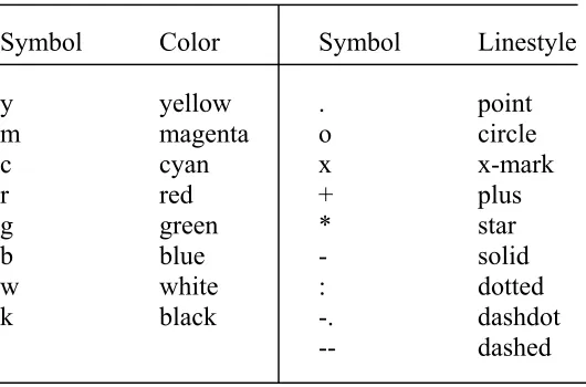
Line styles, markers, and color
Symbol Color Symbol Linestyle
y yellow . point
m magenta o circle
c cyan x x-mark
r red + plus
g green * star
b blue - solid
w white : dotted
k black -. dashdot
-- dashed
Exporting a Figure
1) Cut and paste: click “Edit” at the top menu bar of the figure window, then click “Copy Figure”, paste the figure wherever you want.
2) Save as a file: print –tiff –deps (print as a postscript file). Type “help print” to find out more options.
M-files
MATLAB can execute a sequence of statements in a file. Such files are called “M-files” because they must have the file type of “.m” as the last part of their filename. There are two types of M-files: script files and function files.
Script files
A script file consists of a sequence of normal MATLAB statements. For example, type all the commands for generating the figure into a single script file and save as “sineplot.m”. Then the MATLAB command “sineplot” will cause the statements in the file to be executed. Try it.
You can create new functions specific to your problem, which will then have the same status as other MATLAB functions. Variables in a function files are by default local, otherwise need to be declared as “global”. The function file will start with
function [y1, y2, ..] = Function Name (x1, x2, …)
Here is a simple example. The file myrand.m contains the statements function x = myrand(l, u, row, col)
% generate uniformly-distributed random number matrix (row, col) between low-% bound l and upper-bound u.
x = l + rand(row, col).* (u-l);
We would like to generate a 2 by 3 random matrix between 1.5 and 4.5 » a = myrand(1.5, 4.5, 2, 3)
a =
4.2654 2.0288 4.3064 3.7146 2.7171 4.2507
Numerical Integration / ODE Solver
Numerical Integration (Quadrature) To integrate sin(x) from 0 to pi/4,
» q = quad('sin', 0, pi/4) q =
0.2929
Create an M-file called hump.m function y = hump(x)
y = 1./(x-.3).^2 + .01) + 1./((x-.9).^2 + .04) –7; try out “q = quad(‘hump’, 0, 1)”.
Differential Equation Solver
MATLAB's functions for solving ordinary differential equations are ode23 – 2nd/3rd order Runge-Kutta method
First transform a high-order differential equation into a set of first-order differential equations. Then create a function M-file containing these differential equations. For example,
1 2
2 2 2 1 1
x x
x x 1 x x
=
− − =
&
& ( )
Create a file called “vdpol.m”, function xdot = vdpol(t,x) xdot = zeros(2,1);
xdot(1) = x(1).*(1-x(2).^2)-x(2); xdot(2) = x(1);
To simulate the differential equation defined in “vdpol” over the interval [0,20], invoke ode23
t0 = 0; tf = 20;
x0 = [0 0.25]’; % Initial conditions [t,x] = ode23(‘vdpol’, [t0 tf], x0); plot (t, x)
0 2 4 6 8 10 12 14 16 18 20
-3 -2 -1 0 1 2 3
Type “help ode23” to find out all the other options.
Setting Up Control Systems
Creating transfer function
Consider a single-input single-output system (SISO) given by
) )( . ( ) . ( ) ( 15 s 1 2 s 3 5 s 5 s G + + + =
You can create G(s) using “TF” in MATLAB, » num = 5*[1 5.3];
» den = conv([1 2.1], [1 15]); » sys_1 = TF(num, den)
Transfer function: 5 s + 26.5 --- s^2 + 17.1 s + 31.5
For SISO models, “num” and “den” are row vectors listing the numerator and denominator coefficients in descending powers of s by default.
Creating state space model
Create state-space models in MATLAB is analogous to creating transfer function. Type in A, B, C, D matrices and use command “SS”,
» A = [-23.5 -13.1 -4.5; 1.8 0 0; 0 1 0]; » B = [1 0 0]';
» C = [ 0 18 23]; » D = 0;
» sys_2 = SS(A, B, C, D)
a =
x1 x2 x3 x1 -23.5 -13.1 -4.5 x2 1.8 0 0 x3 0 1 0
b =
c =
x1 x2 x3 y1 0 18 23
d =
u1 y1 0
Transformation between transfer function and state-space models
It is easy to transform a transfer function model into a state-space model, or vice versa. 1) Transform sys_1 from transfer function model to state-space model
» sys_1_ss = SS(sys_1)
a =
x1 x2 x1 -17.1 -3.9375 x2 8 0
b =
u1 x1 4 x2 0
c =
x1 x2 y1 1.25 0.82813
d =
u1 y1 0
2) Transform sys_2 from state-space model into transfer function model » sys_2_tf = TF(sys_2)
Transfer function: 32.4 s + 41.4
Other commands on building models and extract data from a model zpk - Create a zero/pole/gain model.
ssdata - Extract state-space matrices. zpkdata - Extract zero/pole/gain data.
tfdata - Extract numerator(s) and denominator(s).
Computing and Plotting Time Response
For example, we would like to compute and plot step response for a system with no zeros, poles at s= -1+3i and s = -1-3i, and a gain of 3.
» sys_3 = zpk ([], [-1+3*i -1-3*i], 3)
Zero/pole/gain: 3
--- (s^2 + 2s + 10)
» step (sys_3)
Time (sec.)
Amp
lit
ud
e
Step Response
0 1 2 3 4 5 6
0 0.05 0.1 0.15 0.2 0.25 0.3 0.35 0.4
The other commands are
Root Locus Plots
For example, draw root locus plot for a transfer function model9 s 4 s
2 s s
G
2 + + + = ) (
» num =[1 2]; » den = [1 4 9]; » rlocus(num, den)
-6 -5 -4 -3 -2 -1 0 1 2
-2.5 -2 -1.5 -1 -0.5 0 0.5 1 1.5 2 2.5
Real Axis
Im
ag A
xi
s
Find out how to plot root locus for state-space model.
Frequency Domain Plots
Bode Plot
» num =[1 2]; » den = [1 4 9];
Frequency (rad/sec)
P
has
e (
deg)
; M
agn
itud
e (
dB
)
Bode Diagrams
-20 -15 -10
10-1 100 101
-60 -40 -20 0
SIMULINK
SIMULINK is a program for simulating dynamic systems. It has two phases of use: model definition and model analysis. Model definition uses the metaphor of a block diagram, which is much like drawing a block diagram. Instead of drawing the individual blocks, blocks are copied from libraries of blocks. After you define a model, you can analyze it either by choosing options from the SIMULINK menus or by entering commands in MATLAB’s command window. The progress of a simulation can be viewed while the simulation is running, and the final results can be made available in the MATLAB workspace when a simulation is complete.
Open the SIMULINK block library by entering the command » simulink
in the MATLAB command window.
This command displays a new window containing icons for the subsystem blocks
Simulink Block Library 2.2
Copyright (c) 1990-1998 by The MathWorks, Inc. Sources Sinks Discrete Linear Nonlinear
Demos
In1 Out1
Connections
Blocksets & Toolboxes
Example: Building a simple SIMULINK model for a spring-mass-damper system with nonlinear friction.
The spring-mass-damper system is taken from the text book, “Dynamic modeling and control of engineering systems”, Figure 6.6 on Pg. 137.
Open libraries and copy blocks into your model window
Click the window containing icons for subsystem blocks to make it active.
• Double click “Sources”, and then drag “Step” block into your model window from the “Source” library.
• Double click “Linear”, and then drag “Sum” into your model window from the “Linear” library. Double click “Sum”, change “list of signs” to “- +-“.
• Copy two “Gain” blocks from the “Linear” library to your model window, rename one into “Stiffness”, and one to “1/m”. Click the block “Stiffness”, select “flip block” from the “Format” menu to flip the orientation of the block “Stiffness”.
• Copy two “Integrators” blocks from the “Linear” library to your model window, rename one as “Velocity” and one as “Displacement”.
• Double click “Nonlinear”, and then drag “Coulomb” block to your model window from the “Nonlinear” library.
• Double click “Sink”, and then drag “Scope” block to your model window from the “Sink” library, rename the block as “Monitor output”.
Draw lines to connect the blocks
Draw lines to connect the blocks by moving the mouse pointer over a block’s port and holding down the left mouse button. Making a split flow from a connection line is done by pressing the right mouse button and drag the new connection.
s 1
Velocity Sum
1
Stiffness
Step Monitor
ouput s
1
Displacement
Coulomb & Viscous Friction
1
1/m
Change block parameters
• Double click “Stiffness”, set the gain value as 1.0. • Double click “1/m” block, set the gain value as 1.0.
• Double click “Coulomb friction”, set offset as 0.5 and gain as 1.8.
• Double click “Monitor output”, click the “properties” button next to the “print” button, set Ymax as 2.5, and Ymin as –0.5.
• Go back to the model window, select “Parameters” from the “Simulation” menu. Set simulation time: start time = 0.0, and stop time = 5.0
Save the system by selecting “Save” from the “File” menu
Run a simulation by selecting “Start” from the “Simulation” menu
While the simulation is running, the “Start” menu item becomes “Stop”. If you select “Stop”, the menu displays “Start” again.
Click the “Monitor output” block to monitor your system output
Simulation from the Command Line
Any simulation run from the menu can also be run from the command line. For example, use the command
[t, x, y] = rk45(‘model’, [tstart, tfinal]);
where model is the name of the block diagram system you build. Other Ways to View Output Trajectories
Besides using the “Scope” block, output trajectories from SIMULINK can be plotted by • Return variables and the MATLAB plotting commands
References
1) MATLAB User’s Guide, the MathWorks Inc. 2) SIMULINK User’s Guide, the MathWorks Inc.
3) Leonard, N. E. and W. S. Levine, Using MATLAB to Analyze and Design Control Systems, The Benjamin/Cummings Publishing Company, Inc.