Numerical Solutions of Volterra Integral Equations of Second kind with the help of Chebyshev Polynomials

ISSN: 2279-087X (P), 2279-0888(online) Published on 16 November 2012

www.researchmathsci.org

158

Numerical Solutions of Volterra Integral Equations of

Second kind with the help of Chebyshev Polynomials

M. M. Rahman1*_{, M. A. Hakim}4_{, M. Kamrul Hasan}2_{, M. K. Alam}2

and L. Nowsher Ali3

1 _{Department of Mathematics, Islamic University, Kushita-7003, Bangladesh.}

Email: mizan_iu@yahoo.com

2 _{Department of Mathematics & Statistics, Bangladesh University of Business &}

Technology, Dhaka – 1216, Bangladesh.

3_{Department of Electrical and Electronic Engineering, Green University of}

Bangladesh, Dhaka-1216, Bangladesh.

4 _{Department of Mathematics, Comilla University, Comilla, Bangladesh.}

Received 23 September2012; accepted 30 September 2012

Abstract. In the present paper, we solve numerically Volterra integral equations of second kind with regular and singular kernels, by the well known Galerkin weighted residual method. For this, we derive a simple and efficient matrix formulation using Chebyshev polynomials as trial functions. Numerical examples are considered to verify the effectiveness of the proposed derivations and numerical solutions are compared with the existing methods available in the literature.

Keywords: Volterra integral equations, Galerkin method, Chebyshev polynomials. AMS Mathematics Subject Clasifications (2010): 42A10, 42A15

1. Introduction

159

Some valid numerical methods, for solving Volterra equations using various polynomials [2], have been developed by many researchers. Very recently, Maleknejad et al [3] and Mandal and Bhattacharya [4] used Bernstein polynomials in approximation techniques, Shahsavaran [5] solved by Block – Pulse functions and Taylor Expansion method. Taylor polynomials were also used by Bellour and Rawashdeh [6] and Wang [7] with computer algebra. Bernstein polynomials were used for the solution of second order linear and first order non-linear differential equations by Bhatti and Bracken [8]. These polynomials have been also used for solving Fredholm integral equations of second kind by Shirin and Islam [9]. Babolian and Delves [10] describe an augmented Galerkin technique for the numerical solution of first kind Fredholm integral equations. In [11] a numerical solution of Fredholm integral equations of the first kind via piecewise interpolation is proposed. Lewis [12] studied a computational method to solve first kind integral equations.

However, in this paper a very simple and efficient Galerkin weighted residual numerical method is proposed with Chebyshev polynomials as trial functions. The formulation is derived to solve the linear Volterra integral equations of second kind having regular as well as weakly singular kernels, in details, in Section 3. In Section 2, we give a short introduction of Chebyshev polynomials. Finally, five examples of different kinds of Volterra integral equations are given to verify the proposed formulation. The results of each example indicate the convergence numerical solutions. Moreover, this method can provide even the exact solutions, with a few lower order Chebyshev polynomials, if the equation is simple.

2. Chebyshev Polynomials

The general form of the Chebyshev polynomials [12] of nth degree is defined by

∑

1

_! ! _!

1

2

₍₁₎

Using MATLAB code, the first few Chebyshev polynomials from equation (1) are given below:

1 ,

2x 1

4 3

8 8 1

16 20 5

32 48 18 1

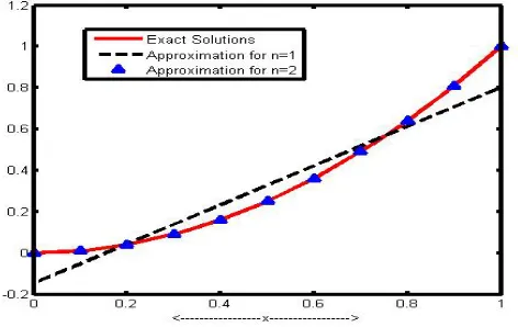
160

Figure 1. Graph of first 6 Chebyshev polynomials over the interval [-1, 1]

3. Formulation of Integral Equation in Matrix Form

We consider the Volterraintegral equation (VIE) of the first kind [6] given by

, ,

2

where is the unknown function, to be determined, , , the kernel, is a continuous or discontinuous and square integrable function, being the known function satisfying 0.

Now we use the technique of Galerkin method, [Lewis, 11], to find an approximate solution of 2 . For this, we assume that

3

where are Chebyshev polynomials of degree defined in equation 1 and are unknown parameters, to be determined. Substituting 3 into 2 , we get

, , 4

161

,

, 5

j=0, 1, 2, … n.

Since in each equation, there are two integrals. The inner integrand of the left side is a function of , and , and is integrated with respect to from . As a result the outer integrand becomes a function of only and integration with respect to from

yields a constant. Thus for each 0, 1, 2, , we have a linear equation with 1 unknowns , 0, 1, 2, , .

Finally 5 represents the system of 1 linear equations in 1 unknowns, are given by

, ; , 0, 1, 2, …

where

, , ,

, 0, 1, 2, ,

,

0, 1, 2, ,

Now the unknown parameters are determined by solving the system of equations

6 and substituting these values of parameters in 3 , we get the approximate solution of the integral equation (2).

Now, we consider the Volterraintegral equation (VIE) of the second kind [6] given by

, ,

7

where is the unknown function to be determined, , , the kernel, is a continuous or discontinuous and square integrable function, and being the known function and is the constant. Then applying the same procedure as described above, we obtain

162

, , , , 0, 1, … ,

where

, 0, 1, 2, … , (8)

Now the unknown parameters are determined by solving the system of equations

8 and substituting these values of parameters in 3 , we get the approximate solution of the integral equation (7). The maximum absolute error for this formulation is defined by

Maximum absolute error | |

4. Numerical Examples

In this paper, we illustrate the above mentioned methods with the help of five numerical examples, which include second kind with regular kernels and weakly singular kernels, available in the existing literature [1- 5]. The computations, associated with the examples, are performed by MATLAB [13, 14]. The convergence of each linear Volterra integral equations is calculated by

δ ϕ

ϕ~ ₁(x) ~ (x)p

E= _n+ − _n

whereϕ~_n(x) denotes the approximate solution by the proposed method using nth degree polynomial approximation andδ varies from ₁₀−6 _for

_n

_≥

₁₀

_.

Example 1. Consider the Volterra integral equations of second kind

x

x

t

x

t

dt

x

)

(

)

(

)

(

0

ϕ

ϕ

=

+

_∫

−

0

≤

x

≤

1

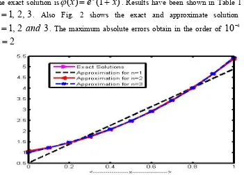
(9)

The exact solution is sin . Results have been shown in Table 1 for

10

,

3

,

1

=

n

. Also Fig. 1 shows the exact and approximate solution for

10

3

,

1

and

163

Figure 2. Exact solution and Numerical solution of example 1 for

n

=

1

,

3

,

10

.

Example 2. Consider the Volterra integral equations of second kind

x

e

t

dt

x x

₍

₎

)

(

0

ϕ

ϕ

=

+

_∫

0

≤x

≤

1

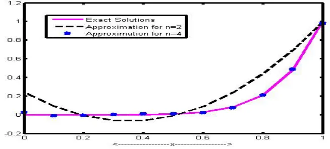
(10)

The exact solution is

ϕ

(

x

)

=

e

x

(

1

+

x

)

. Results have been shown in Table 1 for

3

,

2

,

1

=

n

. Also Fig. 2 shows the exact and approximate solution for

3

2

,

1

and

n

=

. The maximum absolute errors obtain in the order of

10

−4 for

2

=

n

164

Table 1. Computed Absolute Error of examples 1 and 2.

Example 1 for n=10 Example 2 for n=3

Exact Solutions

Approx. Solutions

Absolute Error

Exact Solutions

Approx. Solutions

Absolute Error

0.0 0.0000000 0.0000000 Inf-0.0000000 1.0000000 0.9945330 5.4670224E-003

0.1 0.0998334 0.0998334 2.0508063E-012 1.2156880 1.2167930 9.0893339E-004

0.2 0.1986693 0.1986693 8.3558996E-013 1.4656833 1.4679684 1.5590778E-003

0.3 0.2955202 0.2955202 2.0756558E-013 1.7548164 1.7556648 4.8342409E-004

0.4 0.3894183 0.3894183 2.4960310E-013 2.0885546 2.0874875 5.1090843E-004

0.5 0.4794255 0.4794255 3.6565473E-013 2.4730819 2.4710422 8.2478268E-004

0.6 0.5646425 0.5646425 1.5317015E-013 2.9153901 2.9139342 4.9939072E-004

0.7 0.6442177 0.6442177 1.1908461E-013 3.4233796 3.4237690 1.1375748E-004

0.8 0.7173561 0.7173561 2.5211375E-013 4.0059737 4.0081523 5.4383673E-004

0.9 0.7833269 0.7833269 2.8431391E-013 4.6732459 4.6746893 3.0887023E-004

1.0 0.8414710 0.8414710 8.8095244E-013 5.4365637 5.4309857 1.0260007E-003

Example 3. Consider the Volterra integral equations of second kind

x

x

dt

t

t

x

x

)

3

(

)

3

(

+

_{∫ −}

ϕ

=

ϕ

0

≤

x

≤

1

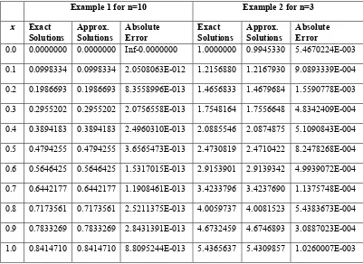
(11)

165

Figure 4. Exact solution and Numerical solution of example 3 for

n

=

2

,

3

Example 4. Consider the weakly singular Volterra integral equations of second kind

)

2

/

1

6435

4096

1

(

7

)

(

2

/

1

)

(

1

)

(

0

x

x

dt

t

t

x

x

_∫

x

=

−

−

−

ϕ

ϕ

0

≤

x

≤

1

(12)

The exact solution is . Using the formula derived in the previous section and solving the system 8 for

n

≥

4

, we get the approximate solution is

, which is the exact solution. On the contrary, the accuracy is found nearly the order of

10

−2 for

n

=

4

in [4].

166

Table 2. Computed Absolute Error of examples 3 and 4.

Example 3 for n=2 Example 4 for n=3

Exact

Solutions Approx. Solutions Absolute Error Exact Solutions Approx. Solutions Absolute Error

0.0 0.0000000 0.0166303 Inf-0.0074113 0.0000000 0.0262542 Inf-0.0074113

0.1 0.1062132 0.1074453 1.1600483E-002 0.0000001 -0.0088862 8.8863240E+004

0.2 0.2258127 0.2193524 2.8608994E-002 0.0000128 -0.0067155 5.2565073E+002

0.3 0.3603635 0.3523517 2.2232608E-002 0.0002187 0.0042983 1.8653831E+001

0.4 0.5116124 0.5064431 1.0103823E-002 0.0016384 0.0101804 5.2136198E+000

0.5 0.6815089 0.6816267 1.7285379E-004 0.0078125 0.0114491 4.6548286E-001

0.6 0.8722292 0.8779024 6.5041788E-003 0.0279936 0.0231158 1.7424592E-001

0.7 1.0862024 1.0952702 8.3481474E-003 0.0823543 0.0746853 9.3122623E-002

0.8 1.3261396 1.3337302 5.7238171E-003 0.2097152 0.2101551 2.0977552E-003 0.9 1.5950668 1.5932823 1.1187893E-003 0.4782969 0.4880164 2.0321071E-002 1.0 1.8963617 1.8739265 1.1830649E-002 1.0000000 0.9812532 1.8746832E-002

Example 5. Consider the weakly singular Volterra integral equations of second kind

1

/

2

15

16

2

)

(

2

/

1

)

(

1

)

(

0

x

x

dt

t

t

x

x

x

_∫

=

+

−

+

ϕ

ϕ

0

≤

x

≤

1

(13)

The exact solution is . Using the formula derived in the previous section and solving the system 8 for 2, we get the approximate solution is , which is the exact solution.

Figure 6. Exact solution and Numerical solution of example 5 for

n

=

1

and

2

5. Conclusions

167

of the polynomials are used in the approximation, which are shown in example 1-5. We also notice that the accuracy increase with increase the number of polynomials in the approximations, which is shown in Table 1 and Table 2. We may realize that this method may be applied to solve other integral equations for the desired accuracy.

REFERENCES

1. Abdul J. Jerri, Introduction to Integral Equations with Applications, John Wiley & Sons Inc., (1999).

2. N. Saran, S. D. Sharma and T. N. Trivedi, Special Functions, Seventh edition, Pragati Prakashan, (2000).

3. K. Maleknejad, E. Hashemizadeh and R. Ezzati, A new approach to the numerical solution of Volterra integral equations by using Bernstein’s approximation, Commun. Nonlinear Sci. Numer. Simulat, 16 (2011), 647-655. 4. B. N. Mandal and Subhra Bhattacharya, Numerical solutions of some classes of

integral equations using Bernstein polynomials, Appl. Mathe. Comput, 190 (2007), 1707-1716.

5. A. Shahsavaran, Numerical approach to solve second kind Volterra integral equations of Abel type using Block-Pulse functions and Taylor expansion by collocation method, Appl. Mathe. Sci., 5 (2011), 685 – 696.

6. Azzeddine Bellour and E. A. Rawashdeh, Numerical solution of first kind integral equations by using Taylor polynomials, J. Inequal. Speci. Func, 1 (2010), 23-29.

7. Weiming Wang, A mechanical algorithm for solving the Volterra integral equation, Appl. Mathe. Comput., 172 (2006), 1323 – 1341.

8. M. Idrees Bhatti and P. Bracken, Solutions of differential equations in a Bernstein polynomial basis, J. Comput. Appl. Mathe., 205 (2007), 272 – 280. 9. A. Shirin and M. S. Islam, Numerical Solutions of Fredholm integral equations

using Bernstein polynomials, J. Sci. Res., 2 (2) (2010), 264 – 272.

10. E. Babolian and L. M. Delves, An augmented Galerkin method for first kind Fredholm equations, Journal of the Institute of Mathematics and Its Applications, 24(2) (1979), 157–174.

11. G. Hanna, J. Roumeliotis, and A. Kucera, Collocation and Fredholm integral equations of the first kind, Journal of Inequalities in Pure and Applied Mathematics, 6(5) (2005), 1–8.

12. B. A. Lewis, On the numerical solution of Fredholm integral equations of the first kind, Journal of the Institute of Mathematics and Its Applications, 16(2) (1975), 207–220.

13. Steven C. Chapra, Applied Numerical Methods with MATLAB for Engineers and Scientists, Second edition, Tata McGraw-Hill, (2007).