Design of LMS Based Adaptive Beamformer for ULA Antennas

71

Design of LMS Based Adaptive Beamformer

for ULA Antennas

Tong Van Luyen

, Truong Vu Bang Giang

1

Hanoi University of Industry, Hanoi, Vietnam

2

VNU University of Engineering and Technology, 144 Xuan Thuy, Cau Giay, Hanoi, Vietnam

Abstract

This paper proposes a design of an adaptive beamformer for arbitrarily Uniformly spaced Linear Array (ULA) antennas. Least Mean Square (LMS), a prevalent adaptive beamforming algorithm, has been employed in the beamformer for the ULA antennas. A procedure has been introduced to validate the proposed design. Applying the proposal, a LMS based adaptive beamformer for 8×1 ULA antennas has been built and implemented on Xilinx FPGA. The fundamental characteristics of the implemented beamformer have been measured and verified. The experimental results show that the beamformer is capable of creating appropriate weights in order to steer the main lobe of the ULA antennas to the desired direction and to place simultaneously null points towards the interferences in case of NOAA LEO satellites system.

Received 01 October 2016, Revised 16 November 2016, Accepted 19 November 2016

Keywords: Beamformer design, Adaptive beamformer, Beamformer implementation, ULA antennas .

1. Introduction*

Adaptive beamfomers utilizing beamforming and beamsteering technique are widely applied for smart antennas. These antennas are very useful to increase the effectiveness of radio spectrum utilizing, interference rejection and reduce power consumption. Indeed, smart antennas are broadly applied in several applications such as radar, sonar, wireless communications, radio astronomy, direction finding, seismology and medical diagnosis and treatment [1]. In terms of operation, the beamformer is based on adaptive beamforming algorithms such as LMS, SMI, RLS, etc. However, in comparison with the others, LMS is a popular adaptive algorithm applying for the beamformer due to some benefits such as simplicity and easily implementing on

_______

*

Corresponding author; E-mail: giangtvb@vnu.edu.vn

hardware, but the disadvantage of this LMS algorithm is slow convergence [2-4].

Recently, design of the beamformer has been extensively studied for a number of applications with several results related to this field from the literature. Design and FPGA implementation of LMS adaptive algorithm for the beamformer have been done by using Xilinx System Generator in [5], however, complete structrure and verification of the beamformer have not been given. In [6], FPGA implementation of a beamformer based on LMS has been built for radar applications. This paper has not presented the design and verification procedure of the implemented beamformer. The work in [7] implemented a LMS based beamformer on FPGA for power analysis of

embedded adaptive beamforming. The

and applied for power analysis of adaptive beamforming.

In our previous papers [8-9], a procedure of designing, verification the beamformer on software has been given. In addition, the design of a beamformer based on FPGA has been shown, but this design has not been implemented and verified on real systems. This is the starting point for further works on the beamformer’s hardware.

In this paper, a design of LMS based adaptive beamformer for arbitrary ULA antennas will be proposed. A procedure for verification of the beamformer will also be introduced. The beamformer will be implemented on Xilinx FPGA and verified in the case of NOAA LEO (National Oceanic and Atmospheric Administration Low-Earth Orbiting) satellites system. The capabilities of forming and steering the beam, operational processes, and convergence characteristics of the beamformer will be verified. The results show that the beamformer operates well in respect of its principal and meets the design’s requirements.

The rest of this paper is organized as follows: Section 2 presents LMS as an adaptive beamforming algorithm for ULA antennas. Design formulation of the adaptive beamformer is introduced in details in Section 3. Section 4 will validate the proposal. Finally, Section 5 will conclude this paper.

2. LMS algorithm for ULA Antennas

The ULA antennas can be constructed by N identical directional elements with the array factor calculated by:

(1)

where is the free space wave number, is the complex weight corresponding to each element, is the

antenna element spacing and is the angle of incidence of incoming signal [10].

Theoretically, if the main lobe of the ULA antennas is steered to direction of the incoming signal, the optimum weights ( ) should be calculated according to mean-squared error (MSE) criterion and can be obtained by Wiener-Hopf equation [10].

(2)

where

is the covariance matrix;

is the cross-correlation vector.

LMS algorithm is invented by Widrow and Hoff in 1960 and has become one of the most widely adaptive algorithms used for filtering [10-11]. The algorithm is based on the steepest-descent method that recursively computes and updates the weight vector based on MSE criterion. MSE is calculated by applying successive corrections to the weight vector in the direction of the negative gradient. The weights can then be updated as

(3)

The algorithm is utilized to compute the instantaneous estimates of and instead of their actual values. Eventually, the calculating steps are as follows:

( 4)

( 5)

( 6)

parameter mainly affects the convergence characteristics of the algorithm.

3. Design Formulation

3.1. Objectives and Requirements This work aims to:

- Design LMS based adaptive beamformer for arbitrary ULA antennas.

- Implement a specific case based on the design, a daptive beamformer for 8×1 ULA antennas, on FPGA.

- Verify the operation of the implemented beamformer in a particular case.

The results are expected to meet some requirements such as:

- The implemented beamformer must work well based on an adaptive beamforming algorithm, LMS algorithm in particular.

- The beamformer can perform main functions such as forming and steering the main lobe to the desired signal, simultaneously placing NULL points toward interferences in case of NOAA satellites system.

3.2. Structure of the beamformer

In this section a structure of the adaptive beamformer based on the foundation given in section 2 and subsection 3.1 will be built. First of all, a flowchart of the LMS based adaptive beamformer is being introduced and presented in Figure 1. Operational principal of the beamformer comprises of following steps:

- Initialization: getting input data such as ; initializing parameters for the beamformer such as index of sampling point ( , total number of samples for processing (no_samples), µ, predefined threshold value

of error ( ), and .

- Matching filter: calculating the cross-correlation of and to detect the reference in the header of wireless communication system frames. Then, if the matching is found, a control signal is generated to enable the LMS algorithm block.

- LMS algorithm: Consecutively calculating three equation (4), (5), and (6) until the error is less than or the number of samples is equal to no_samples.

- Output: Obtaining data of the weights, output signal and error.

Consequently, a structure of the adaptive beamformer has been obtained as given in Figure 2. The beamformer includes four components as WeighMultiplier and Sum, ErrorSubtractor, WeighCalculator, and MatchedFilter.

The MatchedFilter detects the reference in the header of wireless communication system frames. Then, the control signal ( ) is generated to enable the Error Subtractor.

The ErrorSubstractor calculates the difference ( ) between the reference signal and the output signal and gives feedback to the

WeightCalculator by and signal.

N weights ( ) created by

the Weightcalculator have been multiplied by the

input signals ( ) at the

or n = no_samples

Matching

LMS algoritm:

Calculating the equations (4), (5), and (6)

Output:

Weights, output signal and error for step 4

\

Start

TRUE

Intialization: ; parameters: , , , µ, no_samples,

Matching filter:

Cross-correlation of and

TRUE FALSE

FALSE

End

WeightMultiplier to create N sub-products

corresponding to N inputs. These sub-products are added together to give an output signal ( ). e

Figure 2. Structure of the LMS based adaptive beamformer for N×1 ULA antennas.

This beamformer will be implemented on

Virtex 5 FPGA- xc5vsx50t-1ff1136

(XtremeDSP™ Development Kit) by Xilinx ISE 2015.01, and presented in section 4.

3.3. Verification Procedure

Figure 3 gives a procedure of verifying the beamformer, in which following steps are carried out:

- Step 1 - Generating input data:

• Input of signals such as desired signal, interferences, and reference signal.

• Input of parameters such as angle of arrival (AOA) for desired signal, angles of interference (AOI) for interferences, µ for LMS algorithm, and parameters of an 8×1 ULA antenna.

- Step 2 - Creating array response: Getting the output signal ( ) of the array from the data of step 1 using the steering vector.

- Step 3 - Executing beamformer: The beamformer takes input signals from step 2. Then, it utilizes LMS algorithm to produce consecutively updated weights. When the

beamformer gets convergence, these updated weights will be used to form and steer the beam.

- Step 4 - Measuring and verifying: To verify the beamformer, the weights, the output signal, and the error of the beamformer will be measured.

Figure 3. Verification procedure of the beamformer. Step 1: Generating input data

Inputs of signals and parameters Start

Step 2: Creating array response Steering vector

Step 4: Mesuring and Verifying Weights, output signal and error

End

4. Implementation and Experimental Results

Using the above proposals, in this section, the implementation and validation on FPGA of the beamformer will be shown. Following parameters will be used: the processing frequency of 100 MHz (equivalent to a time-unit of 10 ns), µ=0.001, and an ULA antenna array consisting of 8 elements with spacing of λ/2. Each signal is presented in 16 bit fixed-point number. As the results, Xilinx Virtex 5

FPGA resource utilization for the

implemented beamformer is summarized in Table 1. Xilinx chipscope has been used to obtain the measurement data.

Table 1. Virtex 5 resource ultilization for the beamformer

Virtex 5 Resource Used Available Percentage

Number of

Slice Registers 13877 32640 42% Number of LUTs 24183 32640 74% Number of

Occupied Slices 7219 8160 88% Number of

bonded IOBs 20 480 4%

Number of

FG/BUFGCTRLs 1 32 3%

Number of

DSP48Es 132 288 45%

NOAA LEO satellite system has been used to investigate the beamformer following the procedure presented in section 3. In order to do that, the beamformer for 8×1 ULA antennas has been applied for tracking NOAA LEO satellites. The parameters of the satellite communication system, which are given in Table 2, are utilized as input data.

Table 2. NOAA LEO satellite system parameters [12] for verification of the beamformer

Parameters Value

LEO satellite system NOAA

Standard High Resolution

Picture Transmission Type of satellite NOAA KLM and

NOAA-N,-P

Frame format Minor

Reference data for Auxiliary Sync with

beamforming (d(n)) 100 words Noise/Number of

Interferences

AWGN/Up to three interferences Processing time of

the matched filter

315 samples

Processing time of the LMS based beamformer

1685 samples for getting convergence and tracking

There are two scenarios being

investigated: Capability of beamforming and beamsteeting; Convergence characteristics with respect to different SNRs and step-sizes.

a) Capability of beamforming and beamsteeting

Table 3. Parameters for four investigation cases

Cases AOA

(degree)

AOI (degree)

SNR/SIR

Case 1 10 None 30dB

Case 2 -45 0 30dB/10

Case 3 -30 0, 30 30dB/10

Case 4 30 -45,0,50 30dB/10

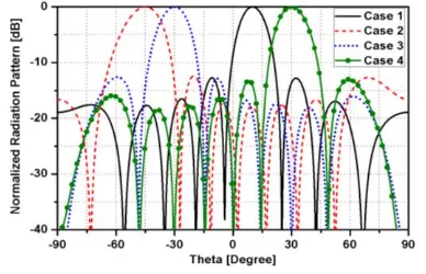
In this scenario, the implemented beamformer has been used to form and steer the beam of the ULA antenna arrays in four cases which have detailed parameters in Table 3. The results including of weights, outputs and errors have been measured and presented.

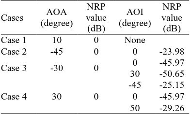
Table 4. Normalized radiation intensities at AOA and AOIs for four investigation cases

Cases AOA

(degree) NRP value (dB) AOI (degree) NRP value (dB)

Case 1 10 0 None

Case 2 -45 0 0 -23.98

Case 3 -30 0 0 -45.97

30 -50.65

Case 4 30 0

-45 -25.15 0 -45.97 50 -29.26

direction and place simultaneously NULL points towards the directions of interferences. Specific values of normalized radiation intensities (NRI) at AOA and AOIs for four cases are shown in Table 4.

For further investigation, weights adaptation, error, output and reference in the case 4 have been presented. The beamforming process for NOAA LEO satellites have been conducted by three periods: matching time for correctly detecting the reference; convergence time for getting the optimized weights according to LMS algorithm; and tracking time for maintaining the state of the pattern. These results have been shown in Figure 5, 6, 7.

Figure 5 presents the measured results of weights, w(n), for eight channels. It can be observed that:

- Weights are zero in matching time because the beamformer is waiting to detect the reference for operation. It takes the matching step 315 time-units to finish.

- Weights strongly vary during the convergence time according to the LMS algorithm.

- Weights are keeping around a mean value with a small variance in tracking time. These weights are stable over time for the rest of time in the reference.

The corresponding error, e(n), is depicted in Figure 6. It can be seen that the convergence time is fewer than 435 time-units at the error less than 0.05.

Figure 7 presents the reference, d(n), and output signal, y(n), over time. It is clear that the beamformer’s output can meet the reference and keep tracking it over time after getting convergence.

Without loss of generality, four cases have been investigated to verify the operation of the beaformer. The results demonstrate that the beamformer is able to form and steer the main lobe to the direction of the desired signal and simultaneously place NULL points to various interferences. Specifically, in the case 4, completed operation of the beamformer has been verified through three periods: matching

time, convergence time, and tracking time. It is clear that the beamfomer operates correctly in respect of the principal given in section 3.

b) Convergence characteristics with respect to different SNRs and step-sizes

Figure 8 gives the error of the beamformer with different SNRs of 10 dB, 20 dB, and 30 dB, respectively, at a fixed step-size µ=0.001. It is clear that the beamformer gets convergence with a nearly constant speed while variance is inversely proportional to SNRs. In addition, the beamformer becomes more stable as the SNR increases.

Figure 9 indicates the error of the beamformer with different step-sizes. It can be observed from Figure 9 that the step-sizes have significant influence on the convergence speed of beamformer. The larger the value step-size is, the faster the convergence but the less the stability around the minimum value is obtained. On the other hand, the smaller the value of step-size is, the slower the convergence but the more stable around the optimum value the beamformer is given.

5. Conclusion

This paper proposed a design of LMS based adaptive beamformer for arbitrary ULA antennas and introduced a verification procedure for the design. In order to validate the design, a beamformer for 8×1 ULA antennas has been implemented on Xilinx FPGA chip. Verification in the case of tracking the NOAA LEO satellites has been done. The measured results show that the beamformer operates well. In particular, the

beamformer is able to form and steer the main lobe to the desired user and simultaneously place NULL points toward various interferences. Besides, it operates correctly in term of the given principal and the LMS algorithm. The proposal

can be applied to design smart antennas for a number of applications such as radar, wireless communications, and directional Wi-Fi.

F

F

H

Figure 6. Error between output and reference signals over time. Figure 5. Weights adaptation over time.

Figure 7. Output and reference signals over time: 0 -1500th

, and 316 - 800th time-unit.

Figure 8. Error over time with different SNRs.

Acknowledgements

This work has been partly supported by Vietnam National University, Hanoi (VNU), under Project No. QG. 16.27.

References

[1] Harry L. Van Trees, “Optimum Array Processing: Part IV of Detection, Estimation, and Modulation Theory”, Chap. 1, pp. 1-12, John Wiley & Sons, 2002.

[2] Constantine A. Balanis, Panayiotis I. Ioannides, “Introduction to Smart Antennas”, Chap. 6, Sec. 6.3, pp. 96-106, Morgan & Claypool, 2007.

[3] Mishra, V., Chaitanya, G., “Analysis of LMS, RLS and SMI algorithm on the basis of physical parameters for smart antenna”, 2014 Conf. on IT in Business, Industry and Government (CSIBIG), pp. 1-4, Indore, India, Mar. 2014.

[4] Senapati, A., Ghatak, K., Roy, J.S., “A Comparative Study of Adaptive Beamforming Techniques in Smart Antenna Using LMS Algorithm and Its Variants”, in Proc. of 2015 International Conf. on CINE, pp. 58-62, Bhubaneshwar, India, Jan. 2015.

[5] A. Reghu Kumar, K. P Soman, Sundaram G. A, “Beam Forming Algorithm Implementation using FPGA”, International Journal of

Advanced Electrical and Electronics Engineering, vol. 2, no. 3, pp. 53-57, 2013. [6] Anjitha D., and Shanmugha S.G.A., "FPGA

Implementation of Beamforming Algorithm for Terrestrial Radar Application”, in Proc. of 2014 International Conf. on Commun. and Signal Processing (ICCSP), pp. 453-457, Melmaruvathur, India, Apr. 2014.

[7] Waheed O.T., Shabra A., and Elfadel I.M., “FPGA Methodology for Power Analysis of Embedded Adaptive Beamforming”, in Proc. of 2015 International Conf. on Commun., Signal Processing, and their Applications (ICCSPA), pp. 1-6,Sharjah, UAE, Feb. 2015. [8] T.V. Luyen, T.V.B. Giang, “Proposal of

Beamformer Hardware Model for Smart Antennas”, in Proc. of The 2014 National Conference on Electronics, Communications and Information Technology, pp. 190-193, Nha Trang, Sep. 2014.

[9] T.V. Luyen, T.V.B. Giang, “Design and Implementation of FPGA based LMS Adaptive Beamformer for ULA Antennas”, in Proc. of The Vietnam Japan Microwave 2015, pp. 71-76, Ho Chi Minh City, Aug. 2015. [10] Jonh Litva, Titus Kwok and Yeung Lo,

“Digital Beamforming in Wireless Communications”, Chap. 2-3, pp. 13-55, Artech House, 1996.

[11] Simon Haykin, “Adaptive Filter Theory”, 5th edition, Chap. 6, pp. 248-308, Pearson, 2014. [12] National Oceanic and Atmospheric

Administration, “The NOAA KLM User's Guide”, Sec. 4.1, pp. 4_1-4_9, Aug. 2014.