Combining time DEA scores using a dynamic panel data model

Int. J. Data Envelopment Analysis (ISSN 2345-458X)

Vol.5, No.2, Year 2017 Article ID IJDEA-00422, 12 pages Research Article

Combining Time DEA Scores Using a

Dynamic Panel Data Model

Geraldo da Silva e Souzaa, Eliane Gonçalves Gomesb*

(a,b) _{Embrapa, Secretaria de Inteligência e Relações Estratégicas – SIRE}

Parque Estação Biológica, Av. W3 Norte final, 70770-901, Brasília, DF, Brazil

Received September, 22, 2016, Accepted March, 25, 2017

Abstract

We define a combined DEA score to evaluate efficiency in agricultural research. The production model we propose considers efficiency measurements under variable returns to scale for each year in the period 2012–2017. We postulate a first-order autoregressive process in the presence of covariates, to explain efficiency. Powers of the autocorrelation coefficient estimated assuming a dynamic panel specification, are used as weights to determine a combined efficiency score. A higher weight is given to recent efficiency measurements. We use a fractional regression model to investigate the statistical significance of covariates on the combined score further.

Keywords: Time series, DEA, Fractional regression, Agricultural research.

*.Corresponding author Email: [email protected]

1. Introduction

Since 1996, the Brazilian Agriculture Research Corporation (Embrapa) has been monitoring the production performance of its research centers by using a Data envelopment analysis (DEA) model [1–5]. Recently, the research centers’ evaluation system has been reviewed, and the efficiency component has gained renewed importance in the whole performance evaluation process. New goals contemplate performance for a time interlude and must accommodate different efficiency components computed within each year.

Current DEA literature includes a plethora of models dealing with the performance measure in a time-series context. The combination with cross-sections is also possible. Malmquist DEA [6] is an instance of DEA analysis for panel data. Lynde and Richmond [7] consider a model for the study of time-series data on inputs and outputs, allowing the inclusion of shifting technology into the DEA framework. Dynamic DEA models and dynamic network DEA models are discussed in Tone [8]. It is not common, however, to model the DEA responses as evolving, satisfying a statistical time-series model where the dependent variable follows a stochastic process. We intend to explore this feature of time-series DEA. We present a method to combine a series of DEA measurements computed in each point in time into a single score, reflecting average efficiency in the period. The method assigns a weight to the efficiency in each year. The weight sequence decreases with time, attributing more importance to recent years by assuming that the efficiency responses, for the panel of decision-making units (DMUs), follow a first-order autoregressive process. The autocorrelation coefficient is estimated by a generalized method of moments (GMM) method [9, 10], assuming a dynamic panel. To the best of our knowledge, the application is new in the DEA context.

Finally, we investigate the effect of contextual classification variables on the efficiency score, with the objective of relating best productions practices with control variables.

2. Production Data

Let

1

0 , 1

j

k

o o

ji ji

i

a a







 be the weights

assigned by unit o within group j for indicator i. There are eight groups, 41 units (research centers), and kj indices for

group j. Let

8

1

0 o, o 1

j j

j

w w







 be the set

of group’s weights for unit o. For period t, let

y

otji denote the value of indicator i for

category j for unit o. Let

y

tji be the mean for period t of attribute i in group j. The output score for unit o for period t is given by:

8

1 1

j

ot

k _ji

ot o o

j ji t

j i

ji

y

y w a

y

 

    _ _ __  

 





(1)

Expenses on labor, capital and other inputs are normalized by the period means and

consider as indices ot ot t

d x

d

 



 , where dot

denotes expenses on item



(labor, capital and other input expenses) by unit o in period t, and dt signifies the average item



expenses in period t. Table 1 shows the input and output data matrices for the year 2012. Type is a categorization of the research centers, based on their research focus: research on agricultural products (Product), on agricultural specific themes (Thematic), and on issues related to environmental and ecological aspects (Ecological), respectively.

Table 1 Production data for 2012

Unit Type X1 X2 X3 Y

DMU_01 Thematic 1.2596 1.6022 1.8564 1.2262

DMU_02 Product 0.9640 0.6145 0.6243 1.8892

DMU_03 Thematic 0.9248 0.8927 1.1162 0.6032

DMU_04 Thematic 1.1331 1.1152 0.3523 0.6292

DMU_05 Product 0.7788 0.7047 0.8194 0.4341

DMU_06 Product 0.9784 1.0158 0.2970 0.2680

DMU_07 Thematic 1.1117 1.1892 1.1169 0.6684

DMU_08 Product 0.9212 0.9100 0.7916 0.3073

DMU_09 Thematic 1.1944 1.2588 1.6828 3.5340

DMU_10 Product 1.1585 1.0735 1.1758 0.8485

DMU_11 Product 0.8747 0.9734 1.3100 0.5487

DMU_12 Product 0.8772 0.5409 1.0461 1.2287

DMU_13 Product 0.7949 0.9082 1.1966 0.8758

DMU_14 Thematic 1.1740 1.1902 1.0041 1.4603

DMU_15 Thematic 1.1367 0.8285 1.5117 1.0967

DMU_16 Product 1.0151 1.2114 0.6319 1.3719

DMU_17 Product 0.9043 0.7265 0.9144 0.6894

DMU_18 Thematic 1.1939 0.7222 0.8624 0.8810

DMU_19 Product 0.9414 1.0763 1.5327 1.3961

DMU_20 Product 0.8337 0.9570 1.3607 1.0567

DMU_21 Product 0.8756 0.7547 0.9975 0.6188

DMU_23 Product 0.9538 1.2033 1.4893 1.1431

DMU_24 Ecological 0.9543 0.7536 0.7585 0.3006

DMU_25 Ecological 0.8879 0.7614 1.0881 0.2147

DMU_26 Ecological 1.0321 1.2781 0.0000 0.0642

DMU_27 Ecological 0.9148 1.0708 1.1193 1.1552

DMU_28 Ecological 1.1476 1.5037 1.1289 0.3723

DMU_29 Ecological 1.1508 1.1897 0.6865 0.4400

DMU_30 Ecological 0.9241 0.7893 0.5842 0.3452

DMU_31 Ecological 1.1111 1.2159 0.8454 0.4286

DMU_32 Ecological 0.8099 0.8341 0.4112 0.3961

DMU_33 Ecological 0.9490 2.4303 0.3894 0.6524

DMU_34 Ecological 0.8915 0.9107 0.8409 0.9681

DMU_35 Ecological 1.1379 0.8255 0.8870 2.3713

DMU_36 Ecological 1.0619 0.8323 0.7585 1.1690

DMU_37 Ecological 0.7845 0.9097 0.7904 0.4018

DMU_38 Ecological 1.0048 0.7678 0.5118 1.4188

DMU_39 Product 0.9722 0.8572 1.2233 1.3563

DMU_40 Product 0.8448 0.7719 2.2280 0.9666

DMU_41 Thematic 1.0975 0.8366 1.9721 0.9905

3. Methodology

The response variable in our analysis is the classical input-oriented DEA measure of technical efficiency, computed under the assumption of variable returns to scale

(DEA-VRS) [12]. If

1 2 41

( , , , )

t t t t

Y  y y y is the output matrix,

and

1 2 41

1 1 1

1 2 41

2 2 2

1 2 41

3 3 3

, , ,

, , ,

, , ,

t t t

t t t t

t t t

d d d

X d d d

d d d

 

 

  

 

 

is the input

matrix, for period t, the DEA-VRS technical efficiency



ˆ

ot for unit o is the solution of the following linear programming problem:

,

1 2 3 1 41

, (

)

(

,

,

)

1,

( ,

,

),

(1,

,1),

0

t ot

t ot ot ot ot ot

i

Min

Y

y

X

x

x

d

d

d

e

e

 





 



























 



(2)

The DEA estimates can be shown to be weakly consistent within years [13]. Under a deterministic frontier assumption in the context of univariate outputs, the DEA estimate is strongly consistent and is a nonparametric maximum likelihood estimate [14. 15]. Assuming independent production decisions under the same production function, these considerations justify the use of DEA responses in regression analysis when covariates are not endogenous or separable [16].

Through time, we assume that the DEA measurements follow the dynamic panel data”:

( 1)

ˆ

ˆ

,

1,..., 41,

2012,..., 2017

ot o t

ot o ot

z

u

o

t

























(3)

centers), and



_ot are iid (independent and identically distributed) errors over the whole sample with constant variance. Both

o

u and



_ot are assumed to be independent for each o over all t. Therefore, the lagged dependent variables are correlated with the unobserved panel level effects, making standard estimation inconsistent [17]. With many panels and few periods, we follow the GMM approach suggested by Arellano and Bover [9] and Blundell and Bond [10]. The model accommodates less restrictive assumptions, regarding the covariates as endogeneity. A key assumption regarding the residual evolution through time is the non-existence of second-order autocorrelation in the differenced series, which can be tested following Arellano and Bond [18]. Exploiting the autoregressive structure, we propose the final efficiency estimate as the following, where



h represents the correlation between efficiencies distant h

periods apart.:

(2017) (2016) 2 (2015) 3 (2014) 4 (2013) 5 (2012)

2 3 4 5

ˆ ˆ ˆ ˆ ˆ ˆ

, 1

1,..., 41

o

o o o o o o

eff o                           _{    }     (4)

Higher-order processes can be considered and tested in the framework of dynamic panels. The correlation structure will be less trivial.

In order to assess the significance of factor variables on the response eff_o, we use a standard fractional regression model [19]. Let an observed response



ˆeff_o with values in (0,1] be dependent on a vector of covariates w. It is assumed that

 

ˆ ( | )

E



w G w



, where G(.) is typically a probability distribution function. The model is well-defined, even when



ˆeff_o

puts positive probability mass at one. The unknown parameter



is then estimated

by quasi-maximum likelihood (QML), maximizing

















1 ˆ log ˆ (1 ) log 1

i i n i i i G w G w       _     _{ }   



[19].

Under the correct specification of the mean function



ˆ



d (0, )

n   N V . V is

estimated as below in (5). The QML estimator is efficient within the class of estimators containing all linear, exponential family-based QML and weighted nonlinear least squares estimators:

 









1 2 1

2 2 2 1

ˆ ˆ

ˆ _{ˆ ,}

ˆ _{1 ˆ} ˆ₍₁ ˆ_{) '}

ˆ ˆ

ˆ _{1 ˆ ˆ ( (1 )) '}

ˆ _{( ' ),} ˆ _{ˆ '( ' ),} ˆ _ˆ ˆ ˆ

n

i i i i i

i

n

i i i i i i

i

i i i i i i i

V A BA

A n g G G w w

B n u g G G w w

G G w  g G w  u  G

           





(5)

These formulas appear in Ramalho et al. [20]. The calculations may be performed with the use of Stata 15 [21], where the method is implemented.

4. Statistical Results

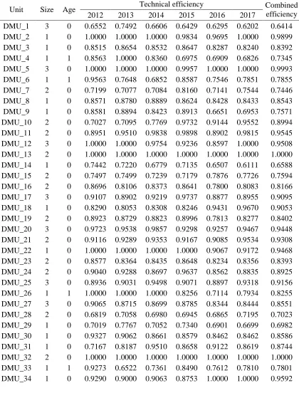
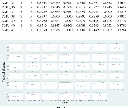
Table 2 shows DEA-VRS efficiency measurements for each year and the combined estimate (column ‘Combined efficiency’). The panel efficiency graphs are shown in Figure 1. One can see that units 2, 5, 13 and 32 are efficient through the period. Units 10, 18 and 34 show an increasing trend. Units 4, 21, 26 and 40 show a decreasing trend. For other units we do not identify a clear trend. The apparent volatility through time calls for an overall measure to capture average performance.

Thematic) and two dummy variables indicating size (base is Large). Research centers were classified into three groups of

size, using cluster analysis (Ward’s method) applied to the evolution of total input expenses.

Table 2: Efficiency scores, age and size (Size: 3 = large, 2 = medium, 1 = small; Age: 0 > 10 years, 1  10 years)

Unit Size Age Technical efficiency Combined

efficiency

2012 2013 2014 2015 2016 2017

DMU_35 1 0 0.8565 0.9069 0.9134 1.0000 0.7691 0.8532 0.8670 DMU_36 2 0 0.8287 0.8046 0.7778 0.8016 0.7977 0.9846 0.8668 DMU_37 3 0 0.9959 0.9869 0.9264 0.9090 0.9245 1.0000 0.9578 DMU_38 3 0 0.9737 1.0000 1.0000 0.9992 0.9259 1.0000 0.9805 DMU_39 1 0 0.8790 0.9583 1.0000 0.9970 0.9155 0.8468 0.9139 DMU_40 1 0 0.9713 0.9147 0.9268 0.9389 0.8243 0.8532 0.8780 DMU_41 2 0 0.7650 0.9288 1.0000 1.0000 0.7149 0.7609 0.8264

Fig. 1

We now analyze the significance of type, size and time effects on the DEA responses. Only a single time dummy was included (2016), to account for a reduction in the overall efficiency level observed in 2016. This effect can be detected by computing the yearly averages (Figure 1). We see that type and size are nonsignificant effects. The results are summarized in Table 3. Exclusion of type and size leads to the final estimates shown

in Table 4. The panel data parameters of Table 4 were used to compute the combined efficiency scores shown in Table 1. We see that the condition for stationarity holds since the autoregressive parameter satisfies

0





ˆ



1

. The Arellano–Bond autocorrelation test has a

Table 3:Preliminary dynamic panel estimation

Coefficient Standard

Error z P>|z|

[95% Confidence Interval]

L1 0.4806 0.1530 3.14 0.002 0.1808 0.7804

Type_Ecological -1.0494 8.5045 -0.12 0.902 -17.7180 15.6192

Type_Product 0.7175 4.9223 0.15 0.884 -8.9301 10.3650

Size_Small -1.9984 11.4951 -0.17 0.862 -24.5284 20.5316 Size_Medium -1.7458 11.3044 -0.15 0.877 -23.9021 20.4105

Time_2016 -0.0504 0.0128 -3.94 0.000 -0.0754 -0.0253

Constant 2.0365 10.0591 0.20 0.840 -17.6790 21.7520

Table 4: Final dynamic panel estimation

Coefficient Standard

Error z P>|z|

[95% Confidence Interval]

L1 0.6643 0.0883 7.53 0.000 0.4913 0.8373

Time_2016 -0.0558 0.0131 -4.25 0.000 -0.0815 -0.0301

Constant 0.3003 0.0759 3.96 0.000 0.1516 0.4490

Arellano–Bond test for zero autocorrelation in first-differenced errors

Order z Prob > z

1 -3.2497 0.0012

2 0.12404 0.9013

H0: no autocorrelation

A joint analysis of type, size and age (a dummy variable indicating whether the research center has been in operation for less than 10 years, age = 1) is then performed by applying fractional regression, assuming the probit or the logistic response to explain the combined efficiency score. The model below assumes the quasi-likelihood function, where





.

is the standard normal or the logistic distribution function;

size

₁

,

size

₂

are dummies for small and medium research centers, and age is the indicator of whether a research center is aged more than 10 years. A further classification of type was considered in the analysis. We do not detect the importance of this effect in the panel regression. The corresponding dummy variables for ecological and product are

type

₁

,

type

₂, respectively. In

the following equation, the betas () are parameters to be estimated:

41 1

0 1 1 2 2 3 4 1 5 2

0 1 1 2 2 3 4 1 5 2

ln

ln

1

(1 ) ln

j j

j

L escore

size size

age type type

size size

escore

age type type

  

  

  

  





    

 

 _{  } 

 

 



 

 _{  } 

 _  _

 

 _{   }

 



(6)

Table 5: Fractional logit regression for combined efficiency score

Coefficient Bias Standard Error

[Bias-corrected 95% Confidence Interval]

Age -0.5922 -0.0191 0.2863 -1.2026 -0.0667

Size_Small -0.2519 -0.0754 0.4474 -1.2010 0.5041

Size_Medium -0.3752 -0.0749 0.4246 -1.2748 0.3363

Type_Ecological 0.6050 -0.0161 0.3232 -0.0410 1.2016

Type_Product 0.9640 0.0030 0.3011 0.3405 1.5174

Constant 1.6077 0.0992 0.5059 0.9684 2.8162

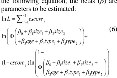
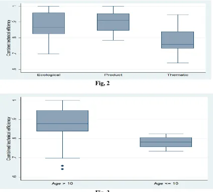
We see significant type and age effects, but not a size effect. Figure 2 and 3 are box-plots describing the observations on the combined efficiency considering, separately, type and age effects. They are not related to the fractional regression

model, but are in close agreement. Comparing the medians (center of the boxes), one can observe the dominance of the Product type and of the older research centers.

Fig, 2

5. Concluding Remarks

We were successful in modeling Embrapa’s production system by applying a deterministic frontier DEA model. The model is justified, given the nature of the response where it is less likely to observe idiosyncratic than deterministic errors. Indeed, a stochastic frontier using the whole sample and a similar specification does not seem to converge.

A better approach was achieved by modeling the DEA time measurements for each research center as a dynamic first-order autoregressive panel, including covariates effects. This idea has appeal since it assumes a common autoregressive coefficient. With only a few time observations for each research center, it is not sensible to estimate separate coefficients. The common estimated autoregressive coefficient is used to define a sequence of weights that decrease over time, reflecting the decreasing importance of lagged efficiency scores. The Arellano– Bond test validates the dynamic model. The final combined scores show a strong association with age and type, but not with the size of a research center. The size of the research center is important since production variables were normalized according to the number of employees, to make units more comparable, reducing unwanted scale effects from potentially biasing the results. Fractional regression consubstantiates this approach.

We also notice from the fractional regression that previous experience with the production evaluation process has a positive effect on the combined efficiency score. It was not possible to include this effect on the dynamic panel, due to collinearities in differences. Research centers classified as Product are more efficient than the others (Ecological and Thematic). This classification of the research centers has been an object of discussion in the company. Based on the fractional regression, we see that in terms

References

[1] Souza GS, Alves E, Avila AFD. Technical efficiency of production in agricultural research. Scientometrics

1999;46(1):141-60. DOI:

10.1007/BF02766299

[2] Souza GS, Gomes EG, Magalhães MC, Avila AFD. Economic efficiency of Embrapa’s research centers and the influence of contextual variables. Pesqui Oper. 2007;27(1):15-26. DOI: 10.1590/S0101-74382007000100002

[3] Avila AFD, Gomes EG, Souza GS, Filho, RCP, de Souza MO. Avaliação de desempenho de unidades de pesquisa agropecuária: métricas e resultados da experiência da Embrapa. Brasília: Embrapa - Secretaria de Gestão Estratégica; 2013. Documentos 16. ISSN: 1679-4680.

[4] Souza GS, Gomes EG. Scale of operation, allocative inefficiencies and separability of inputs and outputs in agricultural research. Pesqui Oper. 2013; 33(3):399-415. DOI: 10.1590/S0101-74382013005000007

[5] Souza GS, Gomes EG. Management of agricultural research centers in Brazil: a DEA application using a dynamic GMM approach. Eur J Oper Res.

2015;240(3):819-24. DOI:

10.1016/j.ejor.2014.07.027

[6] Färe R, Grosskopf S, Norris M. Productivity growth, technical progress, and efficiency change in industrialized countries: Reply. Am Econ Rev. 1997;87(5):1040-43. Available from: http://www.academicroom.com/article/pr oductivity-growth-technical-progress- and-efficiency-change-industrialized-countries

[7] Lynde C, Richmond J. Productivity and efficiency in the UK: a time series application of DEA. Econ Model. 1999;16(1):105-22. DOI: 10.1016/S0264-9993(98)00034-0

[8] Tone, K. Advances in DEA theory and applications: with extensions to forecasting models. Oxford: John Wiley & Sons; 2017.

[9] Arellano M, Bover O. Another look at the instrumental variable estimation of error-components models. J Econom. 1995;68(1):29-51. DOI: 10.1016/0304-4076(94)01642-D

[10] Blundell R, Bond S. Initial conditions and moment restrictions in dynamic panel data models. J Econom. 1998;87(1):115-43. DOI: 10.1016/S0304-4076(98)00009-8

[11] Olesen OB, Petersen NC, Podinovski VV. Efficiency analysis with ratio measures. Eur J Oper Res.

2015;245(2):446-62. DOI:

10.1016/j.ejor.2015.03.013

[12] Banker RD, Charnes A, Cooper WW. Some models for estimating technical scale inefficiencies in data envelopment analysis. Manag Sci. 1984. 30(9):1078-92. DOI: 10.1287/mnsc.30.9.1078

[13] Kneip A, Park BU, Simar, L. A note on the convergence of nonparametric DEA estimators for production efficiency scores. Econom Theory 1998;14(6):783-93. DOI: 10.1017/S0266466698146042

[14] Banker RD. Maximum likelihood, consistency and data envelopment analysis: a statistical foundation. Manag Sci. 1993;39(10):1265-73. DOI: 10.1287/mnsc.39.10.1265

production functions. Braz Rev Econom.

2001; 21(2):291-322. DOI:

10.12660/bre.v21n22001.2753

[16] Simar L, Wilson PW. Two-stage DEA: caveat emptor. J Product Anal.

2011;36(2):205-18. DOI:

10.1007/s11123-011-0230-6

[17] Stata. Stata base reference manual, release 14. College Station, Texas: Stata Press; 2015.

[18] Arellano M, Bond S. Some tests of specification for panel data: Monte Carlo evidence and an application to employment equations. Rev Econ Stud.

1991;58(2):277-97. DOI:

10.2307/2297968

[19] Papke LE, Wooldridge JM. Econometric methods for fractional response variables with an application to 401(k) plan participation rates. J Appl Econom. 1996;11(6): 619-32. DOI:

10.1002/(SICI)1099- 1255(199611)11:6%3C619::AID-JAE418%3E3.0.CO;2-1

[20] Ramalho, E.A., Ramalho, J.J.S., Henriques, P.D. Fractional regression models for second stage DEA efficiency analyses. J Product Anal. 2010;34:239– 255. DOI: I 10.1007/s11123-010-0184-0