Application of charge simulation method to electric field calculation in the power cables

Printed in The Islamic Republic of Iran, 2006 © Shiraz University

"Research Note"

APPLICATION OF CHARGE SIMULATION METHOD TO ELECTRIC

FIELD CALCULATION IN THE POWER CABLES

B. VAHIDI

AND A. MOHAMMADZADEH FAKHR DAVOOD

Tehran, I. R. of Iran, Email: [email protected]

Abstract– Determination of the electric field in insulated cable will lead to an optimum design and a better selection of both conductor size and insulation thickness. A simple numerical method using the Charge Simulation Method (CSM) is used to calculate electric field stresses in high voltage cables. An image charge for each fictitious charge is considered in such a way that the potential of sheath is always kept at zero. The effect of cable sheath is considered and results of the calculation are shown.

Keywords– Three phase cable, field distribution, charge simulation method

1. INTRODUCTION

Insulation strength is limited by the presence of particles and other contamination and voids in synthetic materials. Electrical discharges are initiated in the void or in the vicinity of insulation due to the presence of a localized high electric field. Therefore, the computation of the electric field in a three-core cable is important for the proper design and safe operation of power cables [1-3]. Salama et al. [1] introduced the application of charge simulation method (CSM) for the computation of the electrical field in high voltage cables. In [2] M.Salama and R.Hackam consider a non–shielded insulated conductor placed at a varying distance from a conducting plane using a small number of fictitious charges. In the other paper [1] they used CSM to calculate the electric field in three core belted cables surrounded by a grounded sheath. Salama et al. did not consider the effects of the position of the charges on the accuracy of computation, and this is a weak point of their paper.

Ghourab et al. used optical fiber sensors for online fault and problem detection in an XLPE cable [3]. The insertion of these sensors, which generally possess electrical properties different from those of the cable insulation, is expected to influence the electrical field distribution in the space surrounding the HV conductors. This situation, in turn, affects the electric stress on the HV insulation. This situation is considered in their paper. In the present paper, the electric field at the surface of conductors and on the surface of grounded sheath are obtained using the charge simulation method. The conductors are simulated by an equivalent system of fictituous charges. The method of image generation, in combination with charge simulation, was used to calculate the electric field.

2. CHARGE SIMULATION METHOD (CSM)

The calculation of electric fields requires the solution of Laplace’s and Poissons’s equations with the boundary conditions satisfied. This can be done by either analytical or numerical methods. In many

∗

Received by the editors January 11, 2004; final revised form April 4, 2006.

∗∗

circumstances, the situation is so complex that analytical solutions are difficult or impossible, and hence numerical methods are commonly used for engineering applications. The charge simulation method is one of them [4-7]. This method is simple and accurate.

In a simple example of Fig. 1:

∑

∑

∑

j ij j i

7

1

j i

13

11

j ij j

j ij ) 3 i ( Φ Q P ) 1,2 i ( Φ Q P Q P (1)

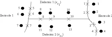
Φi is potential at contour i.

Pij are the potential coefficients.

When boundary condition is applied, a similar condition can be applied to contours on the surface of electrode number 2. In these conditions i and j show the contour number and charge number respectively.

Fig. 1. Typical position of charges and contour points in multi dielectric system (filled circles and stars show charges and contour points respectively)

When the boundary condition is applied for the junction of two insulation: En1 and En2 are normal components of the electric field to the insulation surface.

n2 r2 0 n1 r1

0ε E ε ε E

ε = (2)

Equations are solved to determine unknown charges.

∑

∑

j ij j

j

ijQ P Q 0 (i 8,9,10)

P (3)

⎟ ⎟ ⎠ ⎞ ⎜ ⎜ ⎝ ⎛ + = ⎟ ⎟ ⎠ ⎞ ⎜ ⎜ ⎝ ⎛

∑

∑

∑

j ij j

7

1

j ij j

r2 10

1

j ij j

r1 F Q ε F Q F Q

ε (4)

Fij are field coefficients in a direction which is normal to dielectric boundary at the respective contour points.

In order to determine the accuracy of computation some checkpoints will be considered. By computing the potential in these points and comparing it with actual values, the accuracy of computation will be obtained.

3. USING CSM FOR THE CALCULATION OF THE ELECTRIC FIELD IN THREE CORE BELTED CABLE

The electric field, due to each phase of a three-phase cable, can be simulated by different methods. In this paper, each conductor is represented by an infinite line type charge. For making sheath potential zero, a series of image charges were used.

The worst case was chosen, in which one of the three-phase voltages assumes its peak value. The modeling method for a three-phase cable is shown in Fig. 2 [1].

( )

(

)

(

)

o

120

ωt VCos V

120

-ωt VCos V

ωt VCos V

c b a

+ =

= =

Fig. 2. Modeling of three-phase cable, (1,2,3) are charges, (

1

i

,

2

i

,

3

i

One of the most important problems is finding the exact positions of the image charges. δ is distance of charge location from the center of the conductor. θ is the azimuth angle of the test point.

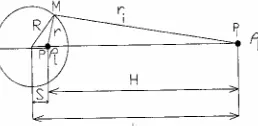
In order to find the exact location of the image charge, Figure 3 has to be considered. In this figure only one phase is shown. Sheath is an equipotential surface with zero value.

If conductor charge and image charge are ρl and ρli respectively (Fig. 3), the location of the image

charge will be determined in a way that makes an equipotential surface (V = 0) with a radius of R.

Fig. 3. Method for finding location of image charge

Potential of a point (M) of this surface is obtained as follows:

r r Ln 2π

ρ

r r Ln 2π

ρ

V 0

0 li

i 0

0 l

M = _ε + _ε (6)

where r0 is the distance of M from reference potential.

For simplicity:

li l =−ρ

ρ Then

r r Ln 2π

ρ

V

i 0 l

M = _ε (7)

In order to delete the effect of r0 , the reference potential point is chosen the same distance from ρl and

S R d_i = 2

Therefore g 2 d T S R , 3 d 2T S S, S R H 2 + + + = + = −

= (8)

For determining the value of the charge, six test points (number of charges) were chosen on conductors and the metal sheath (Fig. 4). In order to check the computation some checkpoints were considered.

Fig. 4. Three-phase cable for showing the location of image charge, checkpoints and test points

To satisfy the boundary condition

[ ][ ] [ ]

Potential coefficients are given by

( )

( )

(

)

(

( )

( )

)

(

)

q P 2 q P

ij Ln X i X j Y i Y j

P = − + − (10)

(Xp, Yp), (Xq, Yq) are coordinates of the test point and test charge location respectively. Similarly, for the electric field:

[ ][ ] [ ]

( )

( )

( )

( )

(

)

(

( )

( )

)

( )

( )

( )

( )

(

)

(

( )

( )

)

q P 2 q P q P Yij 2 q P 2 q P q P Xij j Y i Y j X i X j Y i Y F j Y i Y j X i X j X i X F − + − − = − + − − = (12)

In Fig. 4, points to and to are shown as charge location and image charge location

respectively.

1 to 6 show test points and to are check points. In this figure charges are in the center of conductors (δ=0).

4. RESULTS OF SIMULATION

By using CSM, it is found that the most important parameters in potential and electrical field distribution are T/d and δ/d.

The results of simulation show that error in potential calculation will decrease with increasing T/d ratio. For 1.0 < T/d < 3.0 the error will be less than 0.1%. For this range of potential, the error on sheath will be less than 0.4%.

1 16

These values are for the worst case, (phase angle of conductor A is zero, at time t=0) which in this condition conductor A has the maximum potential.

Figure 5 shows the relation between simulating charges and Τ/d. In Fig. 5, Q are simulating charges and curves are for 0.5 < T/d <3.0. These curves show that Q will increase if T/d decreases.

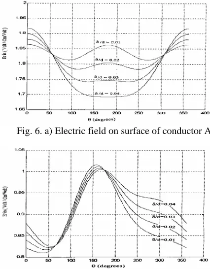
Excessive electric stress can initiate potential discharge and damages the insulation of conductors. Figures 6a, 6b, 6c and 6d show electrical field distribution on the surface of conductors and grounded sheath for different δ/d.

Fig. 5. Effect of Τ/d on value of simulating charge (conductor A)

Figure 6a shows that the electric field increases at a certain point, where the distance between conductor A and sheath has its least value.

Figures 6-b and 6-c show that at 300 and 60 degrees, which are the nearest points to the sheath for conductor B and C respectively, the electric field has its minimum value on the conductors’ surface.

The interesting point is the influence of δ/d on the electric field around the sheath. With increasing δ/d, the electric field around the sheath will decrease, because the charges are far from the sheath, but around the conductors (see Fig. 6d).

Fig. 6. a) Electric field on surface of conductor A Fig. 6. b) Electric field on surface of conductor B

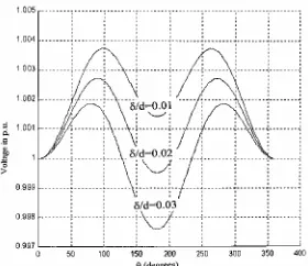
Effect of δ/d on potential distribution is shown in Fig. 7.

5. DISCUSSION

In the present paper, Fig. 7 shows the effect of δ/d on the computation of potential distribution around the conductor, which has one perunit potential (the other two phases have –0.5 p.u. potential). According to Fig. 8, it can be judged that at the point (180 degree) which is close to the sheath when the charge moved far from center of the conductor (greater δ/d), the potential at that point will decrease. By comparing Fig. 5 with Fig. 5 of [1] , Fig. 6a with Fig. 2 of [3] and Fig. 6d with Fig. 4 of [3], the results of the present paper are verified.

Fig. 7. Potential distribution on conductor A versus

θ

Fig. 8. Configuration of conductors in three-phase cable

6. CONCLUSION

In this paper the electric field and potential distribution in a three-phase cable with a grounded sheath have been discussed. As shown in this paper, electric field on conductors and sheath surfaces are not linearly distributed and in some points, the insulation is under more stress. As much as δ/d increases, the potential difference of different points around the conductor will increase (these are not mentioned in other papers). In this paper, the potential around A phase is computed and discussed (these are not mentioned in other papers). In the present paper as well as others, the electric field around phase A, B, C and the effect of δ/d on charge values are discussed. From the results, it can be juged that the maximum electric field in a three core cable occurs at specific locations in the cable.

REFERENCES

1. Salama, M. M. et al. (1984). Methods of calculation of field stresses in a three core power cable. IEEE Trans.

On PAS, PAS-103(12), 3434-3441.

2. Salama, M. M. & Hackam, R. (1984). Voltage and electric field distribution and discharge inception voltage in insulated conductors. IEEE Trans. On PAS, PAS-103(12), 3425-3433.

3. Ghourab, M. E. & Anis, H. I. (1998). Electric stresses in three-core cables equipped with optical sensors. IEEE

Trans. On Dielectrics and Electrical Insulation, 5(4), 589-595.

4. Weifang, J., Huiming, W. & Kuffell, E. (1994). Application of the modified surface charge simulation method for solving axial symmetric electrostatic problems with floating electrodes. Proc. Of 4th int. Conf. On Properties

and Applications of dielectric material, Brisbane, Qld, Australia1, 28-30.

5. Chakravorti, S. & Mukherjee, P. K. (1992). Efficient field calculation in three-core belted cable by charge simulation using complex charges. IEEE Trans. On Electrical Insulation, 27(6), 1208-1212.

6. Malik, N. H. (1989). A review of the charge simulation method and its application. IEEE Trans. On Electrical

Insulation, 24(1), 3-20.

7. Singer, H. et al. (1974). A charge simulation method for the calculation of high voltage fields. IEEE Trans. On