Please cite this article as: H. Nourali, M. Osanloo,A New Cost Model for Estimation of Open Pit Copper Mine Capital Expenditure, International Journal of Engineering (IJE), IJE TRANSACTIONS B: Applications Vol. 32, No. 2, (February 2019) 346-353
International Journal of Engineering
J o u r n a l H o m e p a g e : w w w . i j e . i r
A New Cost Model for Estimation of Open Pit Copper Mine Capital Expenditure
H. Nourali, M. Osanloo*
Department of Mining and Metallurgical Engineering, Amirkabir University of Technology, Tehran, Iran
P A P E R I N F O
Paper history: Received 01 January 2019
Received in revised form 24 January 2019 Accepted 28 January 2019
Keywords:
Capital Expenditure Capital Cost Estimation Mine Investment
Stepwise Multi Varaite Regression
A B S T R A C T
One of the most important issues in all stages of mining study is capital cost estimation. Determination of capital expenditure is a challenging issue for mine designers. In recent decade, quite a few number of studies have focused on proposing estimation models to predict mining capital cost. However, these efforts have not achieved to a predictor model with reliable range of error. Both of overestimation and underestimation of capital expenditure are causing huge problems. The former leads to estimating the value of projects less than the real value, and the latter causes to fail or postpone the project. In this paper, in order to achieve a reliable cost model, the technical and economic data of 15 open pit porphyry copper mines have been collected. The proposed cost model is developed based on stepwise multi variate regression . The R square of the presented model was 97.53% and indicated a proper fit on the data set. In addition, the mean absolute error with respect to the average capital cost of data set used in the modelling procedure was obtained ±8%. The results showed that this model is capable of estimating open pit porphyry copper mine capital expenditure in an acceptable range of error.
doi: 10.5829/ije.2019.32.02b.21
1. INTRODUCTION1
Capital costs are expenditures for the acquisition of property, mineral rights, machinery and for the construction of mines as well as associated infrastructure. These expenditures are typically made once, and are fixed during the life of a mine although some equipment may need to be replaced during a mine’s life [1]. Capital cost estimation is the main part of all stages of mining studies which can play a critical role in deciding about the fate of the project [2-4]. The accuracy of capital expenditure (CAPEX) estimation depends on the level of estimation [3]. Spending capital cost during the early years of mine’s life, has an impressive impact on cash flow of the whole project [5, 6]. Both the overestimation and underestimation of mining CAPEX will create some major problems in the project implementation process. Due to the shortage of data in preliminary stages of project study, the predictor models for CAPEX estimation is often used, but current models cannot predict the mining CAPEX in a reliable range of error [1, 7-10]. Many researchers have tried to develop some cost
*Corresponding Author Email: morteza.osanloo@gmail.com (M. Osanloo)
cases such as estimation of a machine or a product cost [6]. Nevertheless, to estimate the mining CAPEX, several models with a wide range of accuracy have been proposed in the past studies. One of the known methods is the O’Hara model which was developed based on polynomial least square approach [9, 10]. These models were constructed using canadian mining capital cost considering annual ore extraction capasity[23, 24]. Also, Mular [8] presented a rule of thumb for CAPEX estimation, which is called the six-tenths rule. According to Noakes [25] study, this model leads to the results with an error of 30%. In this regard, Wellmer [26] developed a model considering the capacity of mine based on regression method. Camm [7] developed a regression model according to capital cost data of six mines. Long [1] presented a linear, multivariate regression model according to capital cost data collected from 27 porphyry copper ore mine. The following parameters are considered in his study: 1. Mill recovery, 2. Strip ratio, and 3. Distance from the railway station. This model benefited from utilizing other effective parameters in the capital cost estimation, but it still suffered from a wide range of error in CAPEX estimation. Not considering other effective cost drivers such as annual mill production and annual waste stripping in current model causes significant estimation errors. Nevertheless, some of the proposed models can be used for a rough estimation of mining capital cost in the primary stage of mining study. It is clear that to develop a reliable model for capital cost estimation, considering the influence of other effective cost drivers during the model construction process is necessary. In recent decade, the development of machine learning and artificial inteligence based approches has provided powerfull methods to overcome estimation complexity. Accordingly, Nourali and Osanloo [5] presented a regression tree based model for mining CAPEX estimation with acceptable range of errors. In addition, in another research, they proposed other models based on support vector regression theory [6]. In recent studies, the other effective factors such as mine and mill annual production, stripping ratio, reserve mean grade and life of mine are considered in the model construction process which leads to predicting the mining CAPEX for porphyry copper mines with an error range of ±10%. But these models are complicated, and they can not provide an algebraic formula. Regarding the complexity of mining capital cost estimation process, developing a simple, flexible and robust model which can provide a proper estimation under any sophisticated conditions is of great importance. As mentioned above, regression is one of the most famous methods in the cost model construction domain,which has been taken as the foundation of developing a cost model in this paper. To do so, a model is proposed based on the stepwise multivariate regression (SMVR) to estimate the capital cost of mining projects and the capital cost data of 15
porphyry copper ore open pit mine with the same topographical condition are used. In the following sections, preprocessing of data and model construction methodology are described in detail.
2. METHODOLOGY AND DATA SOURCES
One of the applicable methods to develop a predictor model is statistical regression analysis [27]. This technique generates a model based on the relationship between independent input variables, and dependent output variables. The constructed predictor model can estimate the target value according to the input value. The goal is to obtain a reliable generalization; which means that the predictor, calibrated on the basis of a finite set of observed measures, is able to return an accurate prediction of the dependent variable when a previously unseen value of the independent vector appears. Indeed, this method aims to develop a predictor model, according to a set of observations, which is capale of estimating the dependent variable [28]. The most important stage of the model construction is proper predictors selection. Many methods have been proposed to select suitable regressors for model construction. Backward elimination, forward selection, and stepwise regression are classified as the classical methods for this purpose.They sequentially delete or add predictors on the basis of mean squared error or modified mean squared error criteria. Regarding to the ability of these methods, in this research, a stepwise regression method was selected for constructing the cost model.
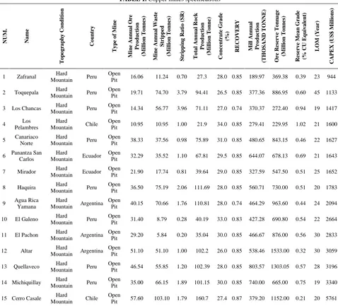
2. 1. Data Set Description To achieve a reliable CAPEX estimator model, the research area should be bounded to the one type of mineral and specific mining method [5, 6]. Therefore, in this paper, the capital cost data of 15 porphyry copper mines and their specifications were collected to construct an estimator model (Table 1). This set of technical and economic data have been gathered by CRU Incorporation. In addition, the capital cost data are escalated to 2016 US dollar [29]. This data set have a wide variation range. To raise the generality of the investigations and globality of developed model, the data set should have a range of dispersion. The descriptive statistics of collected data have been reported in Table 2. This information about the data set indicate that this set of collected data has a suitable dispersion of mining scale. This means that developing a regression model on the basis of this data set can be used for all scale of mining activities.
mill equipment. Accordingly, all of the factors related to production capacity should be considered in cost model
development. Figure 1 illustrates the dependency of each factor with CAPEX.
TABLE 1. Copper mines specifications
TABLE 2. Descriptive Statistics of collected data
Variable Mean StDev Variance Minimum Maximum Median
Mine Annual Ore Production (Million Tonnes) 34.08 15.51 240.52 10.95 64.24 33.65
Stripping Ratio (SR) 1.472 1.078 1.162 0.200 3.960 1.065
Concentrate Grade (%) 28.962 2.222 4.936 26.000 34.000 28.000
Mill Annual Production (THOSAND TONNE) 454.7 172.7 29827.0 190.0 803.6 445.8
Reserve Mean Grade (% CU Equivalent) 0.5521 0.2169 0.0471 0.2083 1.0207 0.5249
LOM (Year) 24.81 6.55 42.96 19.00 45.00 22.50
CAPEX (US$ Millions) 2343 1186 1406901 944 5761 1939
Mine Annual Waste Stripped (Million Tonnes) 46.71 29.44 866.82 5.84 103.10 53.47
Ore Reserve Tonnage (Million Tonnes) 846 434 188125 230 1799 787
N U M . N a me T o p o g ra p h y C o n d it io n C o u n tr y T y p e o f M in e M in e A n n u a l O re Pr o d u ct io n (M il li o n T o n n es) M in e A n n u a l Wa st e S tr ip p ed (M il li o n T o n n es) S tr ip p in g R a ti o ( S R ) T o ta l A n n u a l R o ck Pr o d u ct io n (M il li o n T o n n e) C o n ce n tr a te Gr a d e (%) R E C OV E R Y M il l A n n u a l Pr o d u ct io n (T HO S A N D T ON N E ) Ore R eser v e T o n n a g e (M il li o n T o n n es) R eser v e M ea n Gr a d e (% C U E q u iv a le n t) L OM ( Y ea r) C A PE X ( U S $ M il li o n s)
1 Zafranal Hard
Mountain Peru Open
Pit 16.06 11.24 0.70 27.3 28.0 0.85 189.97 369.38 0.39 23 944
2 Toquepala Hard
Mountain Peru Open
Pit 19.71 74.70 3.79 94.41 26.5 0.85 377.36 886.95 0.60 45 1133
3 Los Chancas Hard
Mountain Peru Open
Pit 14.34 56.77 3.96 71.11 27.0 0.74 370.37 272.40 0.94 19 1417
4 Los Pelambres
Hard
Mountain Chile Open
Pit 10.95 10.95 1.00 21.9 34.0 0.85 279.41 229.95 1.02 21 1600
5 Canariaco Norte
Hard
Mountain Peru Open
Pit 38.33 37.56 0.98 75.89 31.0 0.85 480.65 843.15 0.46 22 1627
6 Panantza San Carlos
Hard
Mountain Ecuador Open
Pit 32.29 35.52 1.10 67.81 29.5 0.85 644.07 678.13 0.69 21 1643
7 Mirador Hard
Mountain Ecuador Open
Pit 21.90 17.74 0.81 39.64 29.0 0.85 327.59 547.50 0.51 25 1652
8 Haquira Hard
Mountain Peru Open
Pit 36.50 75.19 2.06 111.69 28.0 0.85 560.71 730.00 0.51 20 1783
9 Agua Rica Yamana
Hard
Mountain Argentina Open
Pit 40.15 70.66 1.76 110.81 28.0 0.74 464.29 963.60 0.44 24 2094
10 El Galeno Hard
Mountain Peru Open
Pit 31.40 8.79 0.28 40.19 33.0 0.83 427.28 690.80 0.54 22 2664
11 El Pachon Hard
Mountain Argentina Open
Pit 29.20 5.84 0.20 35.04 30.0 0.85 466.67 876.00 0.56 30 2833
12 Altar Hard
Mountain Argentina Open
Pit 51.10 51.10 1.00 102.2 26.0 0.85 538.46 1533.00 0.32 30 3059
13 Quellaveco Hard
Mountain Peru Open
Pit 46.54 55.85 1.20 102.39 28.0 0.85 803.57 1303.05 0.57 28 3196
14 Michiquillay Hard
Mountain Peru Open
Pit 35.00 66.15 1.89 101.15 30.0 0.85 740.00 665.00 0.75 19 3340
15 Cerro Casale Hard
Mountain Chile Open
According to dispersion of data, it is recognized that, the relationship between each cost driver with CAPEX does not follow a particular trend. The amount of R square as the proportion of the variance in the dependent variable -that is predictable from the independent variable - shows that there is not a significant relation between CAPEX and each indipendent variable. Therefore, to develop the reliable cost model the existed data should be preprocessed. To do so, the new CAPEX per tonne of recoverable metal content per year is calculated accorrding to Equation (1).
CPM = CAPEX ÷ (R× MAOP× RMG) (1)
where CPM is CAPEX per tonne of recoverable metal content per year, CAPEX is mining capital cost (US$ Millions), R is mill recovery, MAOP is mine annual ore production, and RMG is reserve mean grade.
In addition, it is suppose that the mill recovery is 100%. Therefore, the total assumed tonnage of concentarte obtained from a given feed, can be calculated by Equation (2).
𝑇𝐶=
𝑅 × 𝑇 𝐹× 𝑔𝐹
𝑔𝐶 (2)
where Tc is the tonnage of concentarate, gc is concentare grade R is mill recovery, Tfis feed tonnage, and gf is feed mean grade. Based on the above calculations, a new data set is prepared for cost model construction (Table 3).
2. 3. Cost Model Development Generally, there are three types of methods of fitting a regression models
with automatic selection of regressor. All of the procedures add or remove any regressors with p-values greater or less than the specified value. These are called Alpha-to-Enter and Alpha-to-Remove value. The first one is forward selection in which all variables not in the model have p-values greater than the specified Alpha-to-Enter value. The second one is backward regression in which all variables in the model have p-values less than the specified Alpha-to-Remove value. The last one is stepwise regression which adds and removes predictors as needed for each step. The procedure stops when all variables not considered in the model have p-values greater than the specified Alpha-to-Enter value and when all variables in the model have p-values less than or equal to the specified Alpha-to-Remove value. Therefore, To develop the cost model, given the ability of mentioned methods, the stepwise regression has been used in the exploratory stages of model building to identify a useful subset of predictors. The process systematically adds the most significant variable or removes the least significant variable during each step. At first, two significance levels should be defined. The first one is Alpha-to-Enter significance level to decide when to enter a predictor into the stepwise model. This is typically greater than the usual 0.05 level so that it is not too difficult to enter predictors into the model. The second one is the Alpha-to- Remove significance level for deciding when to remove a predictor from the stepwise model. This will typically be greater than the usual 0.05 level so that it is not too easy to remove predictors from the model.
(a) (b) (c)
(d) (e) (f)
Figure 1. Dependency of each factor with CAPEX R² = 0.0261
0 0.5 1 1.5 2 2.5 3 3.5 4 4.5
0 1000 2000 3000 4000 5000 6000 7000
S tr ip p in g R a ti o ( S R )
CAPEX (US$ Millions)
R² = 0.1066
0 100 200 300 400 500 600 700 800 900
0 1000 2000 3000 4000 5000 6000 7000
M il l A n n u a l P ro d u ct io n (T H O SA N D T O N N E)
CAPEX (US$ Millions)
R² = 0.2109
0 20 40 60 80 100 120
0 1000 2000 3000 4000 5000 6000 7000
M in e A n n u a l W a st e St ri p p ed ( M il li o n T o n n es )
CAPEX (US$ Millions)
R² = 0.011
25 26 27 28 29 30 31 32 33 34 35
0 1000 2000 3000 4000 5000 6000 7000
C o n ce n tr a te G ra d e ( % )
CAPEX (US$ Millions)
R² = 0.344
0 200 400 600 800 1000 1200 1400 1600 1800
0 1000 2000 3000 4000 5000 6000 7000
O re R e se rv e T o n n a g e (M il li o n T o n n e s)
CAPEX (US$ Millions)
R² = 0.2109
0 20 40 60 80 100 120
0 1000 2000 3000 4000 5000 6000 7000
M in e A n n u a l W a st e St ri p p ed ( M il li o n T o n n es )
TABLE 3. New data set for cost model construction
Consequently, To construct a simple and proper model for mining CAPEX estimation, three below terms have been considered as cost drivers. The following terms are in the fitted equation that models the relationship between Y and the X variables:
CPM: CAPEX per Tonnes of Recoverable Cu Content per Year (US $)
MAWS: Mine Annual Waste Stripped (Million Tonnes) MAOP: Mine Annual Ore Production (Million Tonnes) MLAP100: Mill Annual Production at 100% Recovery (Thousand Tonnes)
If the model fits the data properly, it can be used to predict CAPEX per Tonnes of Recoverable Cu Content per Year (US $) for specific values of the X variables, and can find the settings for the X variables that correspond to a desired value or range of values for CAPEX per Tonnes of Recoverable Cu Content per Year (US $).
To develop a valuable cost model, the relationship between each cost driver and model response must be considered. As it has been showed in Figure 2, the model
response does not significantly have a direct relation with each cost driver.
Regardless of any significant relation among input data and response the stepwise regression methodology was implemented by means of the data set. All the input variables as well as linear and nonlinear compositions of them participated in the modeling procedure. Then the decision of keeping or removing them was made according to the p-values and R square of the model. Figure 3 illustrates the model building sequences displaying the order in which terms were added or removed. The results show that all the three input variables and some of their compositions are considered as the effective variables for model construction. Finally, Equation (3) shows the developed cost model for open pit copper mine capital cost estimation.
𝐶𝑃𝑀 = 27221 − (503 ×
𝑀𝐴𝑊𝑆) − (305 × 𝑀𝐴𝑂𝑃) − (7.5 × 𝑀𝐼𝐴𝑃100) +
(4.97 × 𝑀𝐴𝑊𝑆 2) + (27 × 𝑀𝐴𝑂𝑃2) +
(0.0606 𝑀𝐼𝐴𝑃1002 ) − (2.096 × 𝑀𝐴𝑂𝑃 × 𝑀𝐼𝐴𝑃100
(3)
N
U
M
.
N
a
me
T
o
p
o
g
ra
p
h
y
C
o
n
d
it
io
n
C
o
u
n
tr
y
T
y
p
e
o
f
M
in
e
M
in
e
A
n
n
u
a
l
O
re
Pr
o
d
u
ct
io
n
(M
il
li
o
n
T
o
n
n
es)
M
in
e
A
n
n
u
a
l
Wa
st
e
S
tr
ip
p
ed
(M
il
li
o
n
T
o
n
n
es)
M
il
l
A
n
n
u
a
l
Pr
o
d
u
ct
io
n
A
T
1
0
0
%
R
E
C
OV
E
R
Y
(T
HO
S
A
N
D
T
ON
N
E
)
M
il
l
A
n
n
u
a
l
Pr
o
d
u
ct
io
n
(T
HO
S
A
N
D
T
ON
N
E
)
C
A
PE
X
Pe
r
T
o
n
n
es
o
f
R
ec
o
v
er
a
b
le
C
u
C
o
n
te
n
t
Pe
r
Y
ea
r
(U
S
$
)
1 Zafranal Hard Mountain Peru Open Pit 16.06 11.24 223.49 189.97 17747.26
2 Toquepala Hard Mountain Peru Open Pit 19.71 74.70 443.95 377.36 11330.01
3 Los Chancas Hard Mountain Peru Open Pit 14.34 56.77 501.09 370.37 14170.01
4 Los Pelambres Hard Mountain Chile Open Pit 10.95 10.95 328.72 279.41 16842.09
5 Canariaco Norte Hard Mountain Peru Open Pit 38.33 37.56 565.46 480.65 10919.47
6 Panantza San Carlos Hard Mountain Ecuador Open Pit 32.29 35.52 757.73 644.07 8647.37
7 Mirador Hard Mountain Ecuador Open Pit 21.90 17.74 385.40 327.59 17389.48
8 Haquira Hard Mountain Peru Open Pit 36.50 75.19 659.66 560.71 11356.69
9 Agua Rica Yamana Hard Mountain Argentina Open Pit 40.15 70.66 630.25 464.29 16107.68
10 El Galeno Hard Mountain Peru Open Pit 31.40 8.79 513.37 427.28 18893.52
11 El Pachon Hard Mountain Argentina Open Pit 29.20 5.84 549.02 466.67 20235.70
12 Altar Hard Mountain Argentina Open Pit 51.10 51.10 633.48 538.46 21849.98
13 Quellaveco Hard Mountain Peru Open Pit 46.54 55.85 945.38 803.57 14204.45
14 Michiquillay Hard Mountain Peru Open Pit 35.00 66.15 870.59 740.00 15045.05
C
APE
X
pe
r
T
onne
s
of
R
ec
ove
ra
ble
C
u
C
ontent
pe
r
Ye
ar
(
US
$)
(a) Mine Annual Waste Stripped (Million Tonnes)
(b) Mine Annual Ore Production (Million Tonnes)
(c) Mill Annual Production AT 100% Recovery (Thousand Tonnes) Figure 2. CPM (US $) vs cost drivers
Finally, the total mining CAPEX can be calculated by Equation (4).
𝑇𝑀𝐶 = 𝐶𝑃𝑀 × 𝑀𝐴𝑂𝑃 × 𝑅 × 𝑅𝑀𝐺 (4)
where 𝑇𝑀𝐶is the total mining CAPEX (US$ Millions).
2. 4. Model Evaluation There are several approach to evaluate the goodness of model fitness. The coefficient of multiple determinations R2, and P-value obtained from regression analysis is used as a measure of the capability of explanation of the model. In the presented cost model, the low P-value (<0.001) and high amount of R-square (Rsq=97.53%) show that the developed cost model can estimate mining CAPEX Properly. Moreover, the analysis of the residuals seems as a necessary condition for examining the competency of the model, and outlier examination has been suggested to examine the model stability. There is a wide consensus in taking the root
Figure 3. Model building sequence
mean square error (RMSE) and mean absolute error (MAE) as an essential element to assess a regression model. Therefore, to evaluate the cost model, RMSE, and MAE were calculated by means of Equations (5) and (6). The RMSE shows the difference between inputs and predicted values according to the model.
n y t RSME
n
i i i
1
2
) (
(5)
n
i i
i y
t n MAE
1
1
(6) where tiis the input value, yi is the predicted value and
n is the number of data. By recalling of the evaluation process, the amount of RMSE and MAE of the cost model errors, is reported in the Table 4. In addition, the MAE with respect to the average capital cost of data set used in the modelling procedure was obtained ±8%. Also, Figure 4 indicates the actual CAPEX data versus predicted the same one. It is appear that the proposed model can predict the mining CAPEX of open pit porphyry copper mines in a reliable range of errors.
3. RESULTS AND DISCUSSION
Capital cost is the total cost needed to bring a project to a commercially oerable status. An accurate mining CAPEX estimation pcan guarantee the success of all stage of a mining project excucation. Therefore, according to the different levels of mining study, a reliable CAPEX estimation should be considered. To develop a cost model with acceptable range of error; the
TABLE 4. RMSE and MAE of the cost model errors
Statistical Information Value (CAPEX US$ millions)
RMSE 245.37
(a)CAPEX per tonne of Cu content per year (US$) (b) CAPEX (US$ millions) Figure 4. Performance of the presented model to predict the actual data
collected data should have a wide dispersion, and specificly, should be related to the particular mineral and extarction method [5, 6]. Accordingly, in this paper, a database includs the CAPEX and other technical properties of 15 open pit porphyry copper mines is provided for model construction process. After data preprocessing, CAPEX per tonne of metal content per year was calculated. Then three cost drivers were selected to develop a cost model. With respect to the CAPEX definition, the selected cost drivers are three major components of mining capital cost. The first one is the MAWS (Million Tonnes) that is removal of any waste material in order to access the ore in the deifferent level of open pit mine. The second one is MAOP (Million Tonnes). Both above variables have a direct relation with mining CAPEX. Because increasing the annual tonnage of materials that should be removed leads to an increase in mine fleet size or capacity. The last one is MIAP. This cost driver has a direct relation with mining CAPEX. Increase of mill factory capacity requires more capital cost. With regard to investigations it is recognized that in the stepwise regression analysis the CAPEX per tonne of cu content per year has the best relation with mill annual production at assumed 100 % recovery in the presence of two the other selected cost driver. Therefore, the total supposed mill annual production at 100% recovery was calculated to use in the model construction process. Stepwise regression includes regression models in which the choice of predictive variables is carried out by an automatic procedure. After running a stepwise regression on the data set, a cost model including 3 major varibles was developed. This model fitted on the data with 97% of R square. Model evaluation indices that the proposed cost model can predict the capital cost of open pit porphyry copper mines in an acceptable range of errors.
Regarding to the dispersion of collected, and with respect to the fact that the dataset is assigned to the specific mineral, a new observation most likely lies on this range. For this reason, this regression model is capable to predict the related mining CAPEX in a wide range of mining scale. Furthermore, this algebraic
model can be used in the future resaerch on the copper mine optimisation by means of mathematical modeling.
4. CONCLUSION
Mining CAPEX estimation is a major part of each stage of mining study. With respect to the importance of this issue, many reasearches have been conducted in this area. The estimation error has always been a chalenging issue for mining engineers. To overcome this problem, in this paper, a cost model for estimating mining CAPEX was developed by mean of the stepwise regression analysis. For this purpose, the data of the 15 open pit porphyry copper mine were collected. The most important factors playing significant roles in the capital cost were selected in the stepwise regression procedure. Finally, an algebraic cost model was proposed to estimate open pit pophyry copper mine CAPEX. The results showed that the presented model has a suitable capability in CAPEX estimation with a reliable range of error.
5. REFERENCES
1. Long, K.R., “Statistical methods of estimating mining costs”, In SME Annual Meeting and Exhibit and CMA 113th National Western Mining Conference 2011, Society for Mining, Metallurgy, & Exploration, (2011), 147–151.
2. Mohutsiwa, M., and Musingwini, C., “Parametric estimation of capital costs for establishing a coal mine: South Africa case study”, Journal of the Southern African Institute of Mining and Metallurgy, Vol. 115, No. 8, (2015), 789–797.
3. Shafiee, S., and Topal, E., “New approach for estimating total mining costs in surface coal mines”, Mining Technology, Vol. 121, No. 3, (2012), 109–116.
4. Rahmanpour, M., and Osanloo, M., “Resilient Decision Making in Open Pit Short-term Production Planning in Presence of Geologic Uncertainty”, International Journal of Engineering - Transactions A: Basics, Vol. 29, No. 7, (2016), 1022–1028. 5. Nourali, H., and Osanloo, M., “A regression-tree-based model
for mining capital cost estimation”, International Journal of Mining, Reclamation and Environment, (2018), 1–13. 6. Nourali, H., and Osanloo, M., “Mining capital cost estimation
using Support Vector Regression (SVR)”, Resources Policy, (2018).
0 10000 20000 30000 40000 50000 60000 70000
0 10000 20000 30000 40000 50000 60000 70000
A
ct
u
a
l D
a
ta
Predicted Data
0 1000 2000 3000 4000 5000 6000
0 1000 2000 3000 4000 5000 6000
A
ct
u
a
l
D
a
ta
7. Camm, T.W., The development of cost models using regression analysis, In SME Annual Meeting, Arizona ,(1992).
8. Mular, A.L., “The estimation of preliminary capital costs”, In Mineral Processing Plant Design, New York, SMW/AIME, 1978, Chapter 3, (1978), 52–70.
9. O’Hara, T.A., A Parametric Cost Estimation Method for Open Pit Mines,In Mining Engineering Handbook, Society of mining engineers (SME), New York, (1980).
10. O’Hara, T.A., “Quick Guides to the Evaluation of Orebodies”,
Canadian Institute of Mining Bulletin , Vol. 73, No. 2, (1980), 87–99.
11. Niazi, A., Dai, J.S., Balabani, S., and Seneviratne, L., “Product Cost Estimation: Technique Classification and Methodology Review”, Journal of Manufacturing Science and Engineering, Vol. 128, No. 2, (2006), 563–575.
12. Huang, X.X., Newnes, L.B., and Parry, G.C., “The adaptation of product cost estimation techniques to estimate the cost of service”, International Journal of Computer Integrated Manufacturing, Vol. 25, No. 4–5, (2012), 417–431.
13. Smith, Alice E; Mason, A.K., “Cost estimation predictive modeling: Regression versus neural network”, The Engineering Economist, Vol. 42, No. 2, (1997), 137–161.
14. Daud, B.H., “A Model for Preliminary Evaluation of Underground Coal Mines”, In Computer Methods for the 80’s in the Mineral Industry, Mine Development and Valuation, Society for Mining, Metallurgy, and Exploration, New York, (1979). 15. Petrick, A., and Dewey, R., “Microcomputer cost models for
mining and milling”, In Mineral Resource Management by Personal Computer, Society of Mining Engineers, New York, (1987).
16. Prasad, L., “Mineral processing plant design and cost estimation”, In Processors Division of the Canadian Institute of Mining, Metallurgy and Petroleum, Montreal, (1969). 17. Redpath, J.S., “Estimating pre-production and operating costs of
small underground deposits”, In Canada Centre for Mineral and Energy Technology Minister of Supply and Services Canada, Ottawa, (1986).
18. Stebbins, S., Cost estimation handbook for small placer mines, U.S. Department of the Interior, Bureau of Mines, Pittsburgh, (1987).
19. Sayadi, A.R., Khalesi, M.R., and Khoshfarman Borji, M., “A parametric cost model for mineral grinding mills”, Minerals Engineering, Vol. 55, (2014), 96–102.
20. Arfania, S., Sayadi, A.R., and Khalesi, M.R., “Cost modelling for flotation machines”, Journal of the Southern African Institute of Mining and Metallurgy, Vol. 117, No. 1, (2017), 89–96.
21. Oraee, B., Lashgari, A., and Sayadi, A., “Estimation of capital and operation costs of backhoe loaders”, Society for Mining, Metallurgy & Exploration Annual Meeting & Exhibit and CMA 113th National Western Mining Conference “Shaping a Strong Future Through Mining”, (2011).
22. Sayadi, A.R., Lashgari, A., Fouladgar, M.M., and Skibniewski, M.J., “Estimating Capital and Operational Costs of Backhoe Shovels”, Journal of Civil Engineering & Management, Vol. 18, No. 3, (2012), 378–385.
23. Bertisen, Jasper; Davis, G.A., “Bias and error in mine project capital cost estimation”, The Engineering Economist, Vol. 53, No. 2, (2008), 118–139.
24. Pohl, G., and Mihaljek, D., “Project Evaluation and Uncertainty in Practice: A Statistical Analysis of Rate-of-Return Divergences of 1,015 World Bank Projects”, The World Bank Economic Review, Vol. 6, No. 2, (1992), 255–277.
25. Noakes, M., and Lanz, T., “Cost estimation handbook for the Australian mining industry: MinCost 90”, In Australasian Institute of Mining and Metallurgy, Sydney, (1993).
26. Wellmer, F., Dalheimer, M., and Wagner, M., “Economic evaluations in exploration”, Springer Science & Business Media, (2007).
27. Adalier, O., Uğur, A., Korukoğlu, S., and Ertaş, K., “A New Regression Based Software Cost Estimation Model Using Power Values”, In Intelligent Data Engineering and Automated Learning - IDEAL 2007. Springer Berlin Heidelberg, Berlin, Heidelberg, (2007), 326–334.
28. Bontempi, G., and Kruijtzer, W., “The use of intelligent data analysis techniques for system-level design: a software estimation example”, Soft Computing, Vol. 8, No. 7, (2004), 477–490.
29. Duckworth, D., and John, P.S., “Copper Mine Project Profiles”, 2016 Edition, CRU, London, United Kingdom, (2016).
A New Cost Model for Estimation of Open Pit Copper Mine Capital Expenditure
H. Nourali, M. Osanloo
Department of Mining and Metallurgical Engineering, Amirkabir University of Technology, Tehran, Iran
P A P E R I N F O
Paper history: Received 01 January 2019
Received in revised form 24 January 2019 Accepted 28 January 2019
Keywords:
Capital Expenditure Capital Cost Estimation Mine Investment
Stepwise Multi Varaite Regression
هدیکچ
تاعلاطم یاهشخب نیرتمهم زا یکی م
هژورپ لیبق نیا هیلوا یراذگ هیامرس هنیزه نیمخت ،یندع یم اه
هنیزه نازیم نییعت .دشاب
هیامرس یم رامش هب ندعم نیسدنهم یارب زیگنارب شلاچ لئاسم زا یکی هراومه یا هئارا هنیمز رد یرایسب تاعلاطم ریخا ههد رد .دور
هیامرس هنیزه رگنیمخت یاهلدم م نیا اما .تسا هدش ماجنا یا
.تسا هدشن لوبق لباق یاطخ هدودحم کی اب یلدم هئارا هب رجنم تاعلاط
هیامرس هنیزه نمیخت هدیدع تلاکشم داجیا هب رجنم ،نآ زا رتمک ای و یعقاو رادقم زا شیب یا
یم یندعم هژورپ کی رد یا .ددرگ
کش بجوم نازیم زا رتمک نیمخت و تاعلاطم رد هژورپ شزرا شهاک بجوم دح زا شیب نیمخت دنور نداتفا قیوعت هب ای و تس
هداد ،دامتعا لباق رگنیمخت لدم کی هب یبایتسد روظنم هب ،رضاح قیقحت رد اذل .دیدرگ دهاوخ هژورپ یارجا صتقا و ینف یاه
یدا 51
ماگ هب ماگ شور هب هریغتم دنچ نویسرگر یانبم رب یرگنیمخت لدم ساسا نیا رب .دیدرگ یروآ عمج یریفروپ سم زابور ندعم یم ناشن یزاسلدم دنیآرف زا هدمآ تسدب یگتسبمه بیرض رادقم .دش هداد هعسوت هداد رب یبوخ هب روکذم لدم دهد
ی شزارب اه هتفا
هیامرس هنیزه نیگنایم هب قلطم یاطخ نیگنایم تبسن هولاع هب .تسا هداد یا
رارق هدافتسا دروم یزاسلدم دنیآرف رد هک هیلوا یاه
هتفرگ عم دنا لدا 8 % ± سدب یم ناشن جیاتن .دمآ ت هیامرس هنیزه نیمخت ییاناوت هدش هئارا لدم ،دهد
سم زابور نداعم هیلوا یراذگ