Implementation of a Newton-Krylov Iterative Method to Address Strong Non-Linear Feedback Effects in FORMOSA-B BWR Core Simulator

(1)

Abstract

KASTANYA, DODDY FEBRIAN. Implementation of a Newton-Krylov Iterative Method to Address Strong Non-Linear Feedback Effects in FORMOSA-B BWR Core Simulator. (Under the direction of Paul J. Turinsky.)

A Newton-BICGSTAB solver has been developed to reduce the CPU execution

time of the FORMOSA-B boiling water reactor (BWR) core simulator. The new solver

treats the strong non-linearities in the problem explicitly using the Newton’s method,

replacing the traditionally used nested iterative approach. The Newton’s method provides

the solver with a higher-than-linear convergence rate, assuming that a good initial estimate

of the unknowns is provided. Within each Newton iteration, an appropriately

preconditioned BICGSTAB method is utilized for solving the linearized system of

equations. Taking advantage of the higher convergence rate provided by the Newton’s

method and utilizing an efficient preconditioned BICGSTAB solver, we have developed a

computationally efficient Newton-BICGSTAB solver to evaluate the three-dimensional,

two-group neutron diffusion equations coupled with a two-phase flow model within a

BWR core simulator.

The robustness of the solver has been tested against numerous BWR core

configurations and consistent results have been observed each time. The best exact

Newton-BICGSTAB solver performance, observed when performing calculations on 200

loading patterns (LPs) using an 800 assembly BWR/6 core model, provides an overall

speedup of 2.07 to the core simulator, with reference to the traditional approach, i.e. outer

(2)

traditional approach but with the BICGSTAB solver as the inner iteration solver

[traditional (BICGSTAB)], we observed a speedup of 1.85. This means that the

Newton-BICGSTAB solver provides an additional 12% increase in the overall speedup over the

traditional (BICGSTAB) solver. However, one needs to note that, on average, the exact

Newton-BICGSTAB solver provides an overall speedup of around 1.70; whereas, on

average, the traditional (BICGSTAB) provides an overall speedup of around 1.60.

An investigation on the feasibility of implementing an inexact

Newton-BICGSTAB solver has also been initiated in this research. Results from this study indicate

that further reduction in the execution time can likely be obtained through the

implementation of an inexact Newton’s method. In general, the inexact

Newton-BICGSTAB solver can provide speedups of 1.73 to 2.10 with respect to the traditional

solver. As a specific example, an inexact Newton-BICGSTAB solver, in which the

Jacobian coefficient matrix is approximated and a hybrid Chord-Shamanskii scheme is

used to fix the frequency of the Jacobian matrix updates, can provide 2.10 and 2.27 overall

and solver portion speedups, respectively. For this particular problem where a single LP of

an 800 assembly BWR/6 core model is examined, the speedups gained by utilizing the

traditional (BICGSTAB) solver and by utilizing the exact Newton-BICGSTAB solver are

1.63 and 1.76, respectively. This means that the inexact Newton-BICGSTAB solver

provides additional speedups of 29% and 19% to the traditional (BICGSTAB) solver and

(3)

(4)

“Tersembunyi ujung jalan Hampir atau masih jauh Ku dibimbing tangan Tuhan

Ke negri yang tak ku tau

Bapa ajar aku ikut Apa juga maksudMu Tak bersangsi atau takut

Beriman tetap teguh”

“For my thoughts are not your thoughts, nor are your ways my ways, says the LORD. For as the heavens are higher than the earth, so are my ways higher than your ways

and my thoughts than your thoughts.” Isaiah 55:8-9

(5)

Acknowledgment

The author would like to express his deepest and sincere appreciation to his

advisor, Dr. Paul J. Turinsky, for his invaluable advice, guidance, and mentorship

throughout the preparation of this dissertation. The author also wishes to express his

gratitude for the financial support from the Department of Energy through the Nuclear

Engineering Education Research grant and the Electric Power Research Center at North

Carolina State University. The author also wishes to thank Dr. J. Michael Doster,

Dr. Robert E. White, and Dr. Edward W. Davis, Jr. for serving as his advisory committee

members.

A special thank goes out to his wife, Imelda Ariani, for her love, prayer, patience,

and continuous support. The author would also like to thank his family for their support

(6)

List of Tables

Page

1. Introduction

2. Methodology

Table 2.1. Summary of Time Allocation Study. ...15

Table 2.2. Cases Examined and Stopping Criteria. ...22

Table 2.3. Relative Changes in the Number of Outer Iterations. ...23

Table 2.4. Coupling of Variables. ...26

3. Development of Preconditioners Table 3.1. Preconditioners Performance for a Simplified 368 Assembly BWR/4 Core Model. ...65

Table 3.2. Detail Time Allocation (in seconds1). ...66

Table 3.3. Preconditioner Performance (in seconds1) for a Realistic 368 Assembly GE BWR/4 Core Model. ...69

4. Implementation of BICGSTAB as the Inner Iteration Solver. Table 4.1. R/B LSOR versus BICGSTAB Solvers. ...75

Table 4.2. BICGSTAB Performance for Load Follow Calculations. ...76

Table 4.3. BICGSTAB Performance for Critical Flow Search Calculations. ...78

Table 4.4. FORMOSA-B LP-CRP Optimization Results for SDM Constraint for a 368 assembly GE BWR/4 core. ...79

Table 4.5. FORMOSA-B CRP Sampling Results for an 800 Assembly BWR/6 Core. ...80

5. Results from the Implementation of the Newton-BICGSTAB Solver. Table 5.1. The Newton-BICGSTAB Performance on a Single LP Using True Error Stopping Criteria [Utilizing an 800 Assembly BWR/6 Core]. ...85

Table 5.2. The Newton-BICGSTAB Performance on a Single LP [Utilizing an 800 Assembly BWR/6 Core]. ...86

Table 5.3. CRP Optimization Results Using an 800 Assembly BWR/6 Core. ..92

Table 5.4. Inexact Newton’s Method Results [Utilizing an 800 Assembly BWR/6 Core]. ...93

(9)

Table 5.7. Results from Testing the Hybrid Chord-Shamanskii and Incomplete Jacobian Matrix Approach [Utilizing an 800 Assembly BWR/6 Core]. 99

Table 5.8. Detail Time Allocation from Testing the Hybrid Chord-Shamanskii and Incomplete Jacobian Matrix Approach on a Single LP of 800 Assembly BWR/6 Core. ...100

6. Conclusions and Recommendations for Future Projects.

7. References

Appendix A: Derivation of the Jacobian matrix system for the EPRI void-quality correlation.

(10)

List of Figures

1. Introduction

2. Methodology

Figure 2.1: The traditional nested iterative algorithm. ...13

Figure 2.2: Structure of . ...28

Figure 2.5: Structure of matrix. ...30

Figure 2.6: Structure of the reduced matrix. ...30

Figure 2.7: Linearization error of the k_effvalue. ...33

Figure 2.8: Exact vs. approximate fast flux changes for +10% power perturbation. ...34

Figure 2.9: Discretization notation for the flow channel. ...42

Figure 2.10: The Newton-Krylov algorithm. ...47

Figure 2.11: Exact Newton algorithm. ...50

Figure 2.12: Chord method. ...51

Figure 2.13: Shamanskii’s method. ...52

3. Development of Preconditioners Figure 3.1: Porsching’s algorithm. ...57

Figure 3.2: Structure of Preconditioner Type 1. ...58

Figure 3.3: Preconditioner 1 algorithm. ...59

Figure 3.6: Convergence Behavior of the Preconditioners. ...68

4. Implementation of BICGSTAB as the Inner Iteration Solver. Figure 4.1: Change in unknowns ordering. ...74

Figure 4.2: Optimum CRPs obtained using R/B LSOR inner iteration solver for an 800 assembly BWR/6 core. ...81 Figure 4.3: Optimum CRPs obtained using BICGSTAB inner iteration solver for an

J₂₂

J₂₂iz iz,

J₂₂iz iz, –1 J₂₂

(11)

5. Results from the Implementation of the Newton-BICGSTAB Solver.

Figure 5.1: Newton iterations versus stopping criteria. ...87 Figure 5.2: Multiple LPs results - 800 F/A GE BWR/6 core. ...89 Figure 5.3: Multiple LPs results - 368 F/A GE BWR/4 core. ...90 Figure 5.4: Multiple LP results from testing the hybrid Chord-Shamanskii Method.

...97

6. Conclusions and Recommendations for Future Projects.

(12)

1. Introduction

1.1. Background and Motivation

The arrangement of fuel assemblies and control materials in the core during the

cycle of the nuclear power plant plays an important role in the in-core fuel management.

There are substantial economic benefits that can be derived by optimizing the fuel

assembly and control material loading patterns. At the same time, the desired optimum

fuel assembly and control material loading patterns ought to meet safety and operational

requirements.

Since a typical light water reactor has hundreds of fuel assemblies, evaluating

every possible combinations of loading patterns becomes computationally prohibitive. For

example, a typical pressurized water reactor (PWR) core which has 193 fuel assemblies

will have more than 1050 possible loading patterns to evaluate. In a boiling water reactor (BWR), the type of reactor analyzed in this research, which can contain close to 800 fuel

assemblies and where the positioning of control rods plays an important role in defining a

loading pattern, the number of possible loading patterns increases significantly.

FORMOSA-B [40], which stands for Fuel Optimization for Reloads Multiple

Objectives by Simulated Annealing for BWR, is an in-core nuclear fuel management optimization code which utilizes the simulated annealing (SA) stochastic optimization

method to determine an optimum pairing of loading pattern (LP)- control rod pattern

(CRP) in a BWR. In evaluating the attractiveness of each candidate of LP-CRP pairing

during the course of an optimization, the three-dimensional, two-group neutron diffusion

equation model in conjunction with a two-phase flow model, e.g. three-equation mixture

drift flux model, must be solved as a function of cycle burnup. Consequently, the

associated computational burden for this optimization becomes excessive. For example, a

FORMOSA-B LP-CRP optimization during which approximately 4000 combinations of

(13)

To reduce the CPU time for optimization runs, a Newton type method has been

implemented in the FORMOSA-B code. Through this implementation we try to reduce the

number of iterations required to solve the coupled neutron diffusion and thermal

hydraulics equations by performing simultaneous updates of the flux distribution, the

thermal hydraulics properties, and the k_eff value. We believe that addressing the strong non-linearity in the problem explicitly using the Newton’s method, aided by an

appropriately preconditioned Krylov method for solving the linearized system of

equations within the Newton iteration, should reduce the CPU execution time of an

optimization run. The treatment for the remaining (weaker) feedback mechanisms will be

performed through a nested iterative approach.

Traditionally, the nested iteration approach associated with treating the thermal

hydraulic feedbacks (as well as other feedback mechanisms) has been utilized based upon

the assumption that it is acceptable to delay the iterative update of the thermal hydraulics

feedbacks via updating them at some frequency of the fission source iteration. A more

in-depth discussion about the traditional nested iterative approach is given in Section 2.

Previous studies on Newton type methods within a generalized perturbation theory (GPT)

flux iterative formulation have shown that the Newton’s method is very effective in

treating the thermal hydraulics feedback effects with reference to the rate of convergence

[41].

1.2. FORMOSA-B Code Overview

As briefly indicated earlier, FORMOSA-B is an in-core fuel management code for

BWRs which utilizes the simulated annealing (SA) stochastic optimization method to find

an optimum pairing of LP-CRP. In order to facilitate a proper cooling down schedule for

the SA algorithm, several thousands of LP-CRP pairings are evaluated in each

optimization run. Several objectives are available for the optimization in FORMOSA-B

such as maximization of the end-of-cycle (EOC) core reactivity, minimization of the core

(14)

of the core maximum fraction of limiting critical power ratio (MFLCPR), maximization of

the region average discharge burnup, and minimization of the total reload cost. In addition

to the variety of optimization objectives, FORMOSA-B optimization runs are also

actively controlled by a set of constraints. This set of constraints, which represents the

operating and safety limits, will guarantee that the optimum pairing of LP-CRP obtained

at the end of an optimization, provided that enough pairings have been evaluated and a

feasible solution exists, satisfies the objective of the optimization as well as all of the

constraints.

During an optimization run, it is usually desired to have at least five-to-ten

thousand pairs of LP-CRP evaluated to guarantee a near-optimum solution for the problem

as the result of the optimization. A family of several near optimum pairings of LP-CRP is

also stored in the FORMOSA-B archives file. A core designer could then make his/her

own choice from this pool of solutions.

Although the objective of an optimization makes it unique to other optimizations,

all optimizations share a common thread. In each optimization, FORMOSA-B must

evaluate each pairing of LP-CRP to assess its attractiveness. The evaluation involves

solving the three-dimensional, two-group neutron diffusion equation which is coupled

with a two-phase flow model. It should also be noted that while it is possible to reduce a

PWR model into a two-dimensional model during an optimization run, the strong axial

heterogeneity in a BWR and CRP decisions prevent such simplification.

The coupled neutronics/thermal hydraulics equations are highly non-linear. The

non-linearity is currently treated using a nested iterative technique. More detailed

informations about these nested iterations and the non-linearity of the problem are

discussed in Section 2.

FORMOSA-B can employ either the coarse mesh finite difference (CMFD)

method or the nodal expansion method (NEM) for solving the discretized

three-dimensional problem. Utilizing the NEM as part of the solution technique adds yet another

(15)

1.3. Literature Review

There are abundant sources of information on works related to in-core fuel

management methods for both PWRs and BWRs. A brief review of the historical

approaches to the PWR fuel management outlined in Kropaczek and Turinsky [31] or in

Kropaczek’s dissertation [32] provides a complete discussion in this area. Moore [41]

provides equally comprehensive discussions for the historical development of the BWR

fuel management area in his dissertation. Papers by DeChaine/Feltus [12, 13], Kiguchi

[29], Lin [36], Maldonado/Turinsky [37], Poon/Parks [42], Karve/Turinsky [24], and

Keller/Turinsky [26] are some examples of relatively recent publications which provide

detailed discussions about current practices in the in-core fuel management area.

As mentioned earlier, FORMOSA-B uses the SA method as its optimization

engine. This optimization technique was originally developed based upon the natural

phenomena of slow cooling of a solid. This idea was first introduced by Metropolis et al.

[38] and further refined by Kirkpatrick et al. [30] as a tool for solving optimization

problems. Plethora of sources are available for both the theoretical and application aspects

of the SA method [20, 51, 54, 57]. This optimization technique was first incorporated into

the FORMOSA-P code (an in-core fuel management code for PWRs) by Kropaczek [32]

and then subsequently adopted by the FORMOSA-B code.

The FORMOSA-B code contains the NEM as an option to solve the discretized

three-dimensional problem. Bennewitz [4], Finnemann [18], Wagner [55,56], and Koebke

[55] are some of the pioneers of the NEM. Smith [46] has developed another variant of the

nodal method called the analytic nodal method (ANM) which is characterized by an

analytic solution to the transverse-integrated diffusion equation. Both NEM and ANM are

widely adopted in nuclear reactor core simulator codes [1, 34, 47, 49].

Solution of the neutron diffusion equation, which is a part of the BWR core

simulator, can be written as a solution of a generalized eigenvalue problem. Wachspress

[58] introduced the fission source iteration approach, which is essentially the power

(16)

factor (k_eff), and the associated fundamental mode eigenvector, i.e. the neutron flux ( ), of the generalized eigenvalue problem. This approach is also known as the “outer-inner”

iteration since one will need another “inner” iteration scheme, when working in two or

three dimensional space, for performing the numerical solution of the eigenvector. In

reality, this generalized eigenvalue problem is non-linear since the coefficient matrices are

indirectly dependent upon the eigenvector, i.e. the neutron flux, through directly the flux

or indirectly the power density. One way to treat the non-linearity is to update the

coefficient matrix after several outer-inner iteration sequences and repeat the process until

the eigenvalue, the eigenvector, and the coefficient matrix converge. This idea leads to the

development of the nested iterative approach discussed in Section 2.1.3.

The open literature on the application of Newton’s method for solving the

non-linear two-group neutron diffusion equation problem in a core simulator code is

practically nonexistent. Other than the application of Newton’s type method within the

framework of a GPT flux iterative formulation done by Moore [41], the discussion about

the implementation of Newton’s method in a reactor simulator code as intended in this

research is nonexistent. Therefore, the results of this research should provide significant

contributions in this area to the field of nuclear engineering.

One of the challenges in the implementation of the Newton’s technique in this

research is related to the potential of having a singular matrix at the solution. Since one of

the key assumptions for the Newton’s method is that the Jacobian is not singular at the

solution, we have to ascertain that the singularity of a sub-matrix block does not generate

a singular Jacobian matrix. Fortunately, there have been several studies conducted on this

specific issue. Decker and Kelley provide detailed theoretical discussions for treating

problems related to the singularity of the Jacobian at convergence [14, 15]. In these papers

both exact Newton’s method as well as one type of quasi-Newton’s method, namely the

Broyden’s method, are analyzed.

In recent years, the Krylov subspace methods have begun to be utilized in the core

(17)

domain decomposition preconditioners, into the NESTLE code [52] shows that the

BICGSTAB solver significantly outperforms the line successive over relaxation (LSOR)

method [22, 23] for completing the inner iterations, the method currently used in

FORMOSA-B. Some other recent publications on this subject are available in [17], [21],

[48], and [58].

One of the Krylov subspace methods, e.g. the conjugate gradient squared (CGS),

the BICGSTAB, or the restarted generalized minimal residual (GMRES), will be selected

to be the solver of the linearized system of equations inside each Newton iteration in the

FORMOSA-B code. Discussions about initial developments and some applications of

these Krylov subspace methods can be found in the literatures [5] through [9], [11], [19],

[45], [53]. In addition to these sources, Barrett et al. provides a compact but thorough

discussion on the Krylov methods and also gives some introduction to some families of

preconditioners in [3].

1.4. Purpose and Scope of Research

The objective of this research is to develop a robust and computationally efficient

Newton-Krylov algorithm to solve the three-dimensional, two-group neutron diffusion

equations coupled with a two-phase flow model. This new algorithm has been

implemented in the large-scale in-core fuel management optimization code FORMOSA-B

replacing the currently utilized traditional nested iterative algorithm. The new algorithm

should provide the FORMOSA-B code with the much needed speedup required to make

its usage practical in the design process.

We have formulated and implemented a new algorithm in which the Newton’s

method is utilized to explicitly treat the non-linearities present in the problem. The

associated linearized system of equations represented by the Jacobian matrix system

within each Newton iteration is solved utilizing one of the Krylov methods.

During this research, we have studied the effect of the stopping criteria used for

(18)

and robustness of the solver. We specify these sets of stopping criteria such that the overall

running time is minimized and more importantly that the solver is robust. In addition, the

possibility of implementing an inexact Newton’s method in order to provide an additional

speed up to the code has been initiated.

The last important stage in completing this work is the formulation and

implementation of an appropriate preconditioner to accompany the Krylov solver in order

to minimize CPU time per Newton iteration. In developing the preconditioner, the block

structure of the Jacobian matrix system is fully exploited. Moreover, the preconditioner

also takes advantage of the underlying physics behind the observed structure.

The theoretical aspects of the development of the Newton-Krylov algorithm are

discussed in Section 2. This section summarily introduces the current treatment for the

coupled non-linear neutronics/thermal hydraulics model in the FORMOSA-B code. Also

discussed in this section are the implementations of exact and inexact Newton’s methods,

the derivation of the Jacobian matrix system, and the implementation of a Krylov

subspace solver. This section introduces the Newton-Krylov algorithm.

Section 3 reports the efforts in formulating an appropriate preconditioner for the

Krylov solver. Three types of preconditioners are evaluated representing the evolution of

preconditioners during this research. Two fundamental procedures common to these

preconditioners are also succinctly discussed. Finally, the performance of these

preconditioners are judged and the best one is selected to be implemented in the final

version of the Newton-Krylov solver.

Before evaluating the performance of the Newton-Krylov solver, in Section 4 an

alternative way of providing speedup to the traditional solver is introduced. Implementing

a preconditioned BICGSTAB solver to replace the currently used red/black line SOR

solver as the inner iteration solver proves to provide moderate speedups. Results from

testing this solver on a single loading pattern as well as from optimization runs are

reported in this section.

(19)

traditional solvers for both a single loading pattern case and several optimization runs are

presented in this section.

Finally, Section 6 presents the conclusions regarding this work and provides some

(20)

2. Methodology

2.1. Current Treatment in the FORMOSA-B code

As indicated earlier, during a FORMOSA-B optimization run, we have to evaluate

the dimensional, two-group neutron diffusion equations coupled with the

three-equation mixture drift flux model for the two-phase flow. The first part is called the

neutronics part and the latter part is called the thermal hydraulics part. The neutronics and

thermal hydraulics parts are explained in some details in Section 2.1.1 and Section 2.1.2,

respectively. In the subsequent sub-sections, the non-linearity in this system of equations

will be introduced and the current method used for solving this problem is presented.

2.1.1. Neutronics Model

In order to evaluate the attractiveness of a certain LP-CRP pair, we have to solve

the steady state three-dimensional, two-group neutron diffusion equations. These

equations, assuming no upscatter term, can be written out for a node as follows:

, (2-1)

where:

: diffusion coefficient for neutron energy group ,

: flux for neutron energy group ,

: removal cross section for the fast neutron energy group,

l

D₁( )l ∇φ₁( )l ∇

– +Σ_R1( )l φ₁( )l 1

k_eff

---(νΣ_f1( )l φ₁( )l +νΣ_f2( )l φ₂( )l ) =

D₂( )l ∇φ₂( )l ∇

– +Σ_a2( )l φ₂( )l = Σ_s12( )l φ₁( )l

D_g( )l g

φ_g( )l

g

(21)

: absorption cross section for the thermal neutron energy group,

: scattering cross section from the fast group to the thermal group,

: effective multiplication factor.

Using NEM, we simplify this three-dimensional problem through transverse

integration into three coupled, one-dimensional ordinary differential equations and a nodal

balance equation. The utilization of a nodal methodology when implemented in a

non-linear manner allows us to still employ the same matrix solver technique used in the

coarse mesh finite difference (CMFD) method.

To understand the non-linearity embedded in Eq. (2-1), one needs to realize that

the cross sections ( ) are non-linearly dependent directly on the neutron flux and

indirectly on the power density. The node-wise power density could be expressed as

, (2-2)

where denotes energy released per fission. The direct dependencies of cross sections on

flux are due to transient fission products, e.g. Pm149and Xe135. The indirect dependencies of cross sections on power density are revealed through their dependencies on the

moderator density and fuel temperature. The relationship between these thermal

hydraulics variables to the core power will be explained in Section 2.1.2.

2.1.2. The Thermal Hydraulics Model

The main thrust of this sub-section is to briefly discuss some important aspects of

the thermal hydraulics model utilized in the FORMOSA-B code to the extent that the

discussion provides a clear picture on the relationship between the nodal power and both

the moderator density and the fuel temperature. Discussions about the cross section

dependencies on these thermal hydraulics variables are given in chapter 4 of [41]. Σ_a2( )l

Σ_s12( )l

k_eff

Σ_x

q( )l = κΣ_f1( )l φ( )₁l +κΣ( )_f2l φ₂( )l

(22)

The heart of the two-phase thermal hydraulics model in the FORMOSA-B code is

the three-equation mixture drift flux model. There are several assumptions made in the

implementation of this model. Firstly, it is assumed that the static pressure at the inlet or

the outlet of the flow channels is uniform. Secondly, a subcooled or saturated condition is

assumed at the inlet of a channel, i.e. a fuel bundle. Finally, a one-dimensional, upward

flow is assumed. The last assumption proves to be pertinent in determining the structure of

the linearized system of equations related to the implementation of the Newton’s method.

The full implementation of this model also requires some polynomial fits for the state

equations for both subcooled and saturated conditions to provide the necessary closure of

equations.

The node effective fuel temperature is determined via a polynomial fit of the node

linear power density, , with a correction term to account for fuel exposure,

, expressed as follows

, (2-3)

where denotes the node effective fuel temperature, and denote the

moderator temperature for node and the reference moderator temperature, respectively,

is the linear power density, and is the burnup for node .

While there is a direct expression relating the node relative power to the fuel

temperature, the relation between the node relative power and the node moderator density

is a little bit more arduous to explain. Instead of using complicated formulas to prove a

point that we can indeed relate the node moderator density to the node relative power, the

author chooses to construe the relation by describing the physical phenomena linking the

two.

During a normal operation of a reactor, heat is actively generated inside the core.

This heat will be transferred from the fuel assembly where it is generated to the coolant

(moderator) where the heat is then deposited. Do note that the term coolant and moderator

P q'( ( )l ) ∆T_eff(q'( )l,BU( )l )

T_eff( )l = (T_mod( )l –T_mod(ref))+P q'( ( )l ) ∆+ T_eff(q'( )l,BU( )l )

T_eff( )l T_mod( )l T_mod(ref)

l

(23)

The former expression comes about from the fact that water acts as the convective cooling

media for the core, while the latter one is related to the fact that water moderates the high

energy fission neutrons to lower energies. As heat is added, the water molecules will have

higher energy and will be able to move more freely away from each other. Consequently,

these activities reduce the number of water molecules present in a unit volume of water.

The physical variable representing the total weight of the molecules per unit volume of a

certain substance is called mass density or simply density. Therefore, it should be clear

that the change in the power density distribution, which alters the amount of heat

deposited in the coolant, will have a direct impact on the moderator density.

2.1.3. Traditional Nested Iterative Technique

The traditional method to treat the linearity in the implementation of the

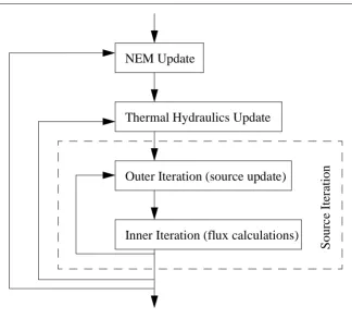
non-linear NEM is to employ a nested iterative algorithm (see Figure 2.1). In the outer most

loop, the spatial coupling coefficients of the NEM are calculated. Inside this loop, the

thermal hydraulics updates are performed. The next inner loop of this nested iterative

algorithm is the source iteration, which consists of yet another level of iterations

(outer-inner iterations). The effective multiplication factor and the fission source term are

updated in the outer iteration. The algorithm will then solve the neutron flux distribution

for both fast and thermal groups via inner iterations. Although we have a coupled system

of equations between the two neutron energy groups, as clearly indicated in Eq. (2-1), we

can solve first the fast group then followed by the thermal group since there is no

upscattering. The Wielandt shift technique, where the eigenvalue of the matrix system is

shifted slightly, is also fully utilized to accelerate the convergence rate of the source

iteration [50]. Since the Wielandt shift technique introduces thermal to fast energy group

coupling, Sutton’s [49] method is employed to remove this coupling. The stopping criteria

for this iterative approach is performed at the outer most level which provides higher

(24)

imposed on the fission source, the effective multiplication factor, and the moderator

density.

The coefficient matrix for each neutron energy group at the inner iteration level

has a seven-banded structure. The system of equations at the inner iteration is solved using

a red/black line successive over relaxation (R/B LSOR) solver with optimum relaxation

parameter values, which are dynamically determined as the coefficient matrix changes due

to non-linear feedback effects or criticality search adjustments.

After obtaining the flux distribution, we can calculate the power distribution inside

the core which is needed to solve for the distributions of the thermal hydraulics properties

of the core. The cross sections are then calculated based upon the updated thermal NEM Update

Thermal Hydraulics Update

Outer Iteration (source update)

Inner Iteration (flux calculations)

Sour

c

e

It

er

ation

(25)

performing the cross section calculation. In addition, we also have enough information to

update the non-linear NEM coupling coefficients. Do note that the thermal hydraulics

updates are performed at a certain frequency of the source iterations and the NEM update

will be done after a certain number of thermal hydraulics updates has been performed. The

frequencies of updates have been studied carefully to determine an optimum combination

of update frequencies which will guarantee the lowest total FLOP count as well as the

robustness of the algorithm.

2.2. Timing Study of the Original FORMOSA-B Code

The purpose of this study is to analyze the performance of the original version of

FORMOSA-B code and to determine where most of the computational time is spent

during an optimization run. There are several objectives which can be selected from for an

optimization run in the FORMOSA-B code. In this study, we have examined four

optimization objectives, namely the EOC k_eff maximization, the maximum fraction of linear power density (MFLPD) minimization, the maximum fraction of limiting critical

power ratio (MFLCPR) minimization, and the region average discharge burnup

maximization. For each of these objectives, we measure the time spent performing five

major functions:

• T/H Calculations: all calculations related to the two-phase mixture drift-flux model.

• Cross Section Calculations: initial cross section setup, cross section updates at each

burnup step, cross section updates due to T/H feedbacks, and fission product feedback

corrections to the absorption cross section.

• NEM Updates: calculating transverse leakages, quadratic expansion coefficients, and

solving the one-node/two-node problems.

• Coefficient Matrix Setup: setting up the coefficient matrix for solving the

generalized eigenvalue problem .

• Linear Equation Solver: completing the inner iterations using the R/B LSOR solver.

M

(26)

The results from this study are summarized in Table 2.1. Before analyzing the results, do

note that each optimization run examines approximately 8,000 loading patterns with a

fixed control rod pattern.

From Table 2.1, one can see that for all optimization objectives, approximately

40% and 90% of the total execution time is spent in the linear equation solver and in the

overall solver, respectively. This implies that if time spent for the linear solver could be

made close to zero, we could speedup the code by only a factor of around 1.6. To obtain

higher speedup, we need to seek other sources of speedup which will significantly reduce

not only the linear solver time but more importantly the overall solver time. Implementing

the Newton’s method, which is capable of updating several non-linear feedback properties

simultaneously, is the path taken to provide the needed speedup.

Table 2.1: Summary of Time Allocation Study.

FORMOSA-B Function

Optimization Objective

EOC k_eff maximization

MFLPD minimization

MFLCPR minimization

Region average discharge BU maximization

T/H Calculations

18.80% 18.84% 21.06% 20.02%

Cross Section Calculations

13.60% 16.41% 15.56% 14.52%

NEM Updates 12.71% 12.82% 14.45% 13.49%

Coefficient Matrix

Setup

4.38% 4.47% 5.05% 4.84%

Linear Solver 43.04% 40.67% 36.48% 38.77%

(27)

2.3. Implementation of Newton’s Method

This section is further divided into five sub-sections. In the first two sub-sections,

a brief discussion on the mathematical background of the Newton’s method and results

from studies performed to determine strong non-linear feedback mechanisms are

presented. A direct application of the Newton’s method to the problem at hand is also

concisely discussed. The next sub-section covers the system of equations involved in the

model. The structure of the Jacobian matrix system is observed in the ensuing sub-section.

This sub-section also discusses how the Jacobian matrix system is simplified by reducing

the number of unknowns in the system. Finally, the last sub-section presents results from

the linearization error study.

2.3.1. Mathematical Background

Consider a non-linear equation given by

, (2-4)

where the non-linear operator operates on the unknown vector whose vector

dependence indicates different reactor core properties. Eq. (2-4) includes appropriate

boundary conditions and, if an eigenvalue problem is involved, normalization constraint.

For the problem at hand, the unknown vector consists of all of the unknowns and can

be subdivided into the eigenvalue ( ), where , the neutron group flux ( ), the

strong non-linear feedback properties ( ), i.e. fuel temperature, coolant temperature, and

coolant density, and the weak non-linear feedback properties ( ), i.e. Xe135and Sm149 number densities and nodal spatial coupling correction coefficients. The unknown vector

can be mathematically written as

. (2-5)

A( )Φ = Q

A Φ

Φ

λ λ = 1 k⁄ _eff φ

ξ

Ψ

(28)

The subdivision of the non-linear feedback properties is performed in order to allow

different iterative update frequency between the strong and the weak feedback properties.

A study for determining which feedback mechanisms are considered strong has been

completed and the results are presented in Section 2.3.2. Expressing Eq. (2-4) explicitly in

terms of the eigenvalue, neutron flux and feedback properties, we obtain

. (2-6)

The first row of Eq. (2-6) indicates the balance equation for the neutron flux, i.e. the

spatially discretized form of the three-dimensional, two-group neutron diffusion equation.

The and denote the loss and production operators, respectively. Note that these

operators are independent of flux. The second row of Eq. (2-6) represents some form of

two-phase fluid mass, energy, and momentum conservation equations, such as the

commonly employed drift-flux model, along with the constitutive equations which are

used to determine the coolant density distribution in the core, plus the core power level

normalization constraint. The third row states the balance equations for the weak

non-linear feedback properties.

The traditional nested iterative algorithm for solving Eq. (2-6), as visualized in

Figure 2.1, can be mathematically written as

, for , (2-7)

, for , (2-8)

and

, for , (2-9)

where , , and denote the fission source, strong non-linear feedback properties, and

A( )Φ

M(ξ Ψ, ) λ– F(ξ Ψ, )

( )φ

Tˆ(φ ξ Ψ, , ) W(φ ξ Ψ, , )

0

Qˆ_ξ

0

= =

M F

M(ξ_n,Ψo)φm+1–λmF(ξn,Ψo)φm = 0 m = 0 1 2, , ,…

Tˆ(φm˜,ξn+1,Ψo) = Q_ξ n = 0 1 2, , ,…

W(φ_m, ,ξ_n Ψo+1) = 0 o = 0 1 2, , ,…

(29)

on top of or underneath them indicate the frequency of updates; for example, several

fission source iterations could be performed prior to updating the strong non-linear

feedback properties.

Ideally, it is desired to update the flux and the strong non-linear feedback

properties simultaneously. This can be done through a Newton type method [27, 28]. The

implementation of Newton’s method in the FORMOSA-B code will be focused only on

treating the neutron flux and strong non-linear feedbacks properties. The remaining

(weak) non-linear feedbacks will be updated in an iterative fashion as an additional loop

outside the Newton iteration loop.

The non-linear system of equations we are interested in solving by the Newton’s

method can be written as

. (2-10)

The core power level constraint equation has been separated out of the operator in

Eq. (2-10), with the operator denoting the strong feedback properties. As noted earlier,

since an eigenvalue equation is being solved, a constraint equation is required, in this case

to normalize the flux. The constraint equation allows the eigenvalue to be introduced as an

additional unknown. The exact Newton equation for non-linear equation, Eq. (2-10),

suppressing the dependence upon the weak non-linear feedbacks, , which are updated in

an outer iterative loop, can be expressed as

, (2-11)

where the Jacobian matrix has been defined as

, (2-12)

B( )Θ

M(ξ Ψ, ) λ– F(ξ Ψ, )

( )φ

T(φ ξ Ψ, , ) κΣ_f,φ

〈 〉

≡ = Q

0

Q_ξ Q_P ≡

Tˆ

T

Ψ

J(Θm)Θm+1 = R(Θm)

J(Θm) Θ ∂

∂ B( )Θ

Θm

(30)

, (2-13)

and

, (2-14)

and index denotes the Newton iteration count. For our problem, the Jacobian matrix

can be written as

. (2-15)

Eq. (2-15) denotes a 3x3 block matrix whose block matrix components are denoted by

for . Using Eq. (2-11) and Eq. (2-15), one obtains the iterative

algorithm (in similar fashion to Eqs. (2-7) through (2-9)) as follow

, (2-16)

, (2-17)

and

Θm φm T

ξm T

λ_m

, ,

[ ]T

≡

R(Θ_m)≡J(Θ_m)Θ_m–(B(Θ_m)–Q)

m

J(Θm)

M( ) λξ – F( )ξ

[ ]

ξ ∂

∂

M( ) λξ ξ ∂

∂ F( )ξ

–

 

 _φ _–_F_{( )φ}_ξ

φ ∂

∂

T(φ ξ, )

ξ ∂

∂

T(φ ξ, ) 0

φ

∂∂ κΣ〈 f,φ〉 _∂∂ κΣ_ξ〈 f,φ〉 0

Θm =

J(Θm)i j, i j, = 1, 2, 3

J(Θm)1 1, φm+1+J(Θm)1 2, ξm+1+J(Θm)1 3, λm+1 =

J(Θm)1 1, φm+J(Θm)1 2, ξm+J(Θm)1 3, λm

( )–

M( ) λξ_m – _mF( )ξ_m

[ ]φm

J(Θm)2 1, φm+1+J(Θm)2 2, ξm+1 =

J(Θm)2 1, φm+J(Θm)2 2, ξm–[T(φm,ξm)–Q_ξ]

(31)

Reintroducing the weak non-linear feedback values, they are determined by solving for

using

. (2-19)

This set of equations is clearly more difficult to solve than the original matrix

equations associated with the traditional nested iterative approach due to the simultaneous

couplings of more unknowns. However, the Newton’s method is still attractive since it

converges to the solution at a-higher-than-linear rate provided that a good initial guess of

unknown values is used. Kelley provides copious discussion on the convergence behavior

of the exact Newton’s method in his book [27]. Discussion on the rate of convergence for

the inexact Newton’s method can be found in [16].

2.3.2. Non-linear Feedback Study

As indicated in the previous section, the non-linear feedbacks are categorized into

strong and weak ones. Therefore, prior to implementing the Newton-Krylov solver into

the FORMOSA-B code, we investigated the strengths of the non-linearities in the systems

of equations solved. We would like to precisely identify the strong non-linear feedbacks

for which a Newton-type treatment is more computationally advantageous than the

currently utilized nested iteration algorithm.

To answer this question, we have performed a comprehensive study to determine

which feedback mechanisms can be categorized as strong feedbacks. If the total number of

outer (fission-source) iterations increases noticeably when a non-linear feedback effect is

treated, then the feedback is categorized as a strong feedback. The non-linear feedbacks

associated with the thermal hydraulics, coolant inlet flow redistribution, transient fission

products, and the non-linear nodal iterative method spatial coupling correction

coefficients have been examined. The behaviors of the non-linear feedbacks on four core

types, namely a 368 assembly GE BWR/4 core, an 800 assembly GE BWR/6 core, a 724 Ψ

(32)

assembly GE BWR/3 core, and a 560 assembly GE BWR/4 core, have been evaluated to

verify the consistency of the results.

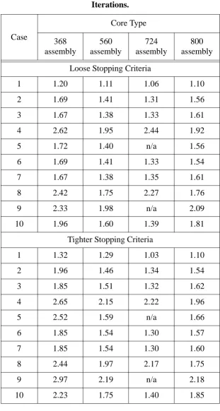
Table 2.2 presents the cases examined during this study and the stopping criteria

utilized. The results of this study are summarized in Table 2.3. Included in this table are

results from performing the study using two different sets of stopping criteria. The cases

examined are chosen such that the individual effect of a certain feedback can be isolated

(cases 1, 2, 3, and 5) as well as the aggregate effect of several feedbacks (cases 4 and 6

through 10). Note that the ratio is defined as

, (2-20)

where denotes the number of outer iterations for a particular combination of

non-linear feedbacks being tested and denotes the number of outer iterations without

nodal, thermal hydraulics, coolant inlet flow redistribution, and critical flow search

feedbacks treated.

Averaged over the four core types for Case 1, utilization of the NEM in place of

the CMFD method increases the number of outer iterations on average by 12% and 19%

for the loose and tighter stopping criteria, respectively. Due to these moderate changes in

the number of iterations, this feedback mechanism is categorized as a weak feedback.

Case 2 shows the effect of thermal hydraulics feedback without flow

redistribution, critical flow search, and spacer void model. Averaged over four core types,

this feedback effect is considered a strong feedback mechanism since it increases the

number of outer iteration by around 50%, regardless of the stopping criteria employed.

Comparing the ratio values for Cases 2 and 3, one can see that performing the inlet

flow redistribution, such that the core has uniform inlet and outlet pressures for all flow

channels, does not significantly change the number of outer iterations. Similar observation

can also be made on Cases 6 and 7, where the nodal method is utilized for solving the

Ratio nouter

Case

n_outerRef

---=

n_outerCase

(33)

Table 2.2: Cases Examined and Stopping Criteria.

Case NEM TH Flow

Redistribution

Critical Flow

Spacer Void

Fission Product

1 On Off Off Off Off

On

2 Off On Off Off Off

3 Off On On Off Off

4 Off On On On Off

5 Off On Off Off On

6 On On Off Off Off

7 On On On Off Off

8 On On On On Off

9 On On On On On

10 On On On On Off Off

Stopping Criteria

; ;

Note: and are the two consecutive outer most loop iterations.

Loose Stopping Criteria 5e-4 1e-4 5e-2

Tighter Stopping Criteria 1e-4 5e-5 2e-4

k_eff( )q –k_eff(q–1) k_effq

---≤ε_k ρ q

( ) _ρ(q–1)

– 2

ρ( )q

2

---≤ε_ρ [Fφ] q ( )

Fφ [ ](q–1)

– 2

Fφ [ ]( )q 2

---≤ε_F

q q–1

(34)

Table 2.3: Relative Changes in the Number of Outer Iterations.

Case

Core Type

368 assembly

560 assembly

724 assembly

800 assembly

Loose Stopping Criteria

1 1.20 1.11 1.06 1.10

2 1.69 1.41 1.31 1.56

3 1.67 1.38 1.33 1.61

4 2.62 1.95 2.44 1.92

5 1.72 1.40 n/a 1.56

6 1.69 1.41 1.33 1.54

7 1.67 1.38 1.35 1.61

8 2.42 1.75 2.27 1.76

9 2.33 1.98 n/a 2.09

10 1.96 1.60 1.39 1.81

Tighter Stopping Criteria

1 1.32 1.29 1.03 1.10

2 1.96 1.46 1.34 1.54

3 1.85 1.51 1.32 1.62

4 2.65 2.15 2.22 1.96

5 2.52 1.59 n/a 1.66

6 1.85 1.54 1.30 1.57

7 1.85 1.54 1.30 1.60

8 2.44 1.97 2.17 1.75

(35)

Observing the ratio values of Cases 3 and 4 as well as Cases 7 and 8, one can see

that the critical flow search feedback mechanism can actually be categorized as a strong

feedback. This feedback adds 9% to 83% increase in the number of outer iterations on top

of the already strong thermal hydraulics feedbacks. However, in this research the critical

flow search feedback will be treated in a nested iterative fashion with other weak

feedbacks.

Although employing the spacer void model does not change the number of outer

iteration considerably, it will still be treated using the Newton’s method since the spacer

void model directly affects the coolant density distribution which is a part of the thermal

hydraulics model. Finally, comparing the ratio values of Cases 10 and 8, with the

exception for the 724 assembly GE BWR/3 core, the fission product feedback causes

moderate changes in the number of outer iteration and, hence, is categorized as a weak

feedback.

Based on these results, we concluded that the thermal hydraulics feedbacks are

considered strong feedbacks and, therefore, their associated unknowns will be treated

using the Newton’s method. The remaining weak feedbacks will be treated in a nested

iterative fashion.

2.3.3. System of Equations

To fully understand the complexity in solving the coupled matrix equations (Eq.

(2-16), Eq. (2-17), and Eq. (2-18)), one needs to examine the components of this matrix

system. Extended discussion on the basic equations composing the three-equation mixture

drift flux model used in the FORMOSA-B code can be found in Moore’s dissertation [41]

and will not be repeated here. Based on these equations, we can derive the Jacobian matrix

(36)

2.3.4. Structure of the Jacobian Matrix System and Equation Reduction

Assuming that a three-equation, two-phase drift flux model is utilized, the strong

non-linear feedbacks can be written as follow

, (2-21)

where: is the void fraction,

, and is the fuel temperature,

is the moderator density,

and are mixture void-quality parameters,

is the flow quality,

is the quality at net vapor generation,

is the equilibrium quality,

is the mixture internal energy,

is the mixture pressure, and

is the mixture mass flux.

Table 2.4 shows the coupling for the neutron flux and the strong non-linear

feedback properties, where an X denotes a coupling in the governing equations. The

relations shown represent the couplings when the Lellouche-Zolotar EPRI void-quality

correlation is utilized. The couplings shown in this table represent all possible couplings

between the variables regardless of the condition of the fluid. Reduced couplings exist for

single-phase flow or two-phase flow where thermal equilibrium exists. One more

important thing to note about this table is the fact that while the variables’

inter-dependencies are nicely visualized, the additional complexities regarding the spatial

coupling between nodes have not been revealed yet.

ξ = [αT, , ,ZT ρT C₀T,V_gjT,x_fT,x_nvgT,x_eqT, ,uT PT,GT]T

α

Z≡ T_f T_f ρ

C₀ V_gj

x_f

x_nvg

x_eq

(37)

Following the notations in Eqs. (2-16) through (2-18), we can symbolically write

the linearized system of equations to be solved as:

, (2-22)

where , , and denote the changes in successive Newton iterative values, e.g.

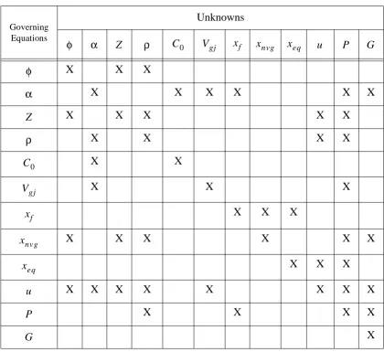
. Before discussing the method for solving this system of equations, we Table 2.4: Coupling of Variables.

Governing Equations

Unknowns

X X X

X X X X X X

X X X X X

X X X X

X X

X X X

X X X X X X

X X X

X X X X X X X X

X X X X

X

φ α Z ρ C₀ V_gj x_f x_nvg x_eq u P G

φ α

Z ρ

C₀

V_gj

x_f

x_nvg

x_eq

u P G

J11 J12 J13 J21 J22 0

J31 J32 0 δφ δξ δλ

R₁ R₂ R₃

=

δφ δξ δλ

(38)

would like to observe the structure of the block sub-matrices. Since the Krylov technique

will be utilized to solve this system of equations, the information about the structure of the

block sub-matrices is crucial in developing the preconditioner to accompany the Krylov

solver.

The sub-matrix represents the Jacobian of the discretized three-dimensional,

two-group neutron diffusion equation and has a seven-block-banded structure. Note that

unlike the treatment in the traditional solver, both energy groups are solved

simultaneously producing the 2x2 block structure. The structure of sub-matrix

suggests that a family of Block Incomplete LU (BILU) Decomposition could be utilized

as part of the preconditioner.

The structure of the matrix will be examined next. First note that since BWRs

employ closed flow channels and inlet flow redistribution is not being treated by the

Newton’s method, all flow channels are decoupled at the Newton iterative level. This

implies that each flow channel can be treated separately. The general structure of for a

flow channel can be seen on Figure 2.2, where denotes the bottom node and

denotes the top node.

Note that the sub-matrix represents the Jacobian of the thermal hydraulics

equations at axial node with respect to the thermal hydraulics properties of axial node

, and the sub-matrix represents the Jacobian of the thermal hydraulics

equations at the axial node with respect to the thermal hydraulics properties of axial

node . Also note that in this analysis, the thermal hydraulics variables are arranged

as follow:

. (2-23)

J₁₁

J₂₂

iz = 1

iz = NZ

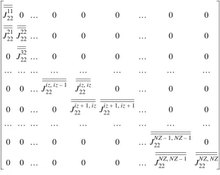
J₂₂iz iz,

iz

iz J₂₂iz iz, –1

iz iz–1

ξ ( )iz

αiz

Ziz ρiz C₀iz V_gjiz xiz_f x_nvgiz x_eqiz uiz Piz Giz

[ ]T

(39)

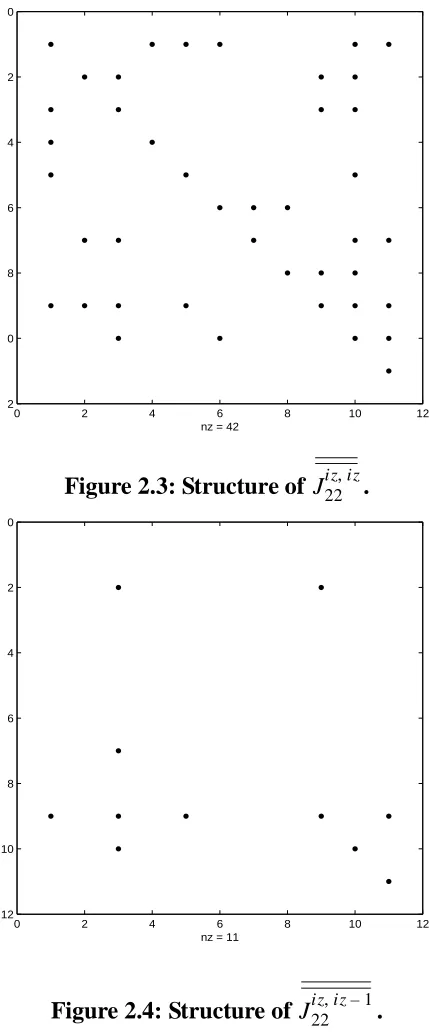
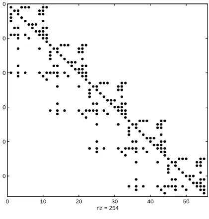
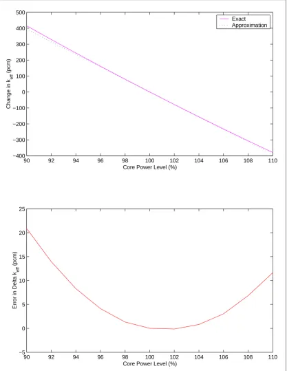
The structures of and are shown in Figures 2.3 and 2.4, respectively.

Using this information, we can visualize the structure of the overall matrix,

which is shown in Figure 2.5 for an example where the z-line has five axial nodes. Note

that in solving Eq. (2-22), the Jacobian matrix of the coupled thermal hydraulics

equations, which consist of eleven variables, are algebraically reduced to four equations

and four unknowns (i.e., pressure, density, internal energy, and void fraction) per axial

node. The structure of the reduced system of equations is shown in Figure 2.6, again

assuming five axial nodes.

Since each block of the reduced matrix is a 4-by-4 matrix, the inverse of each

diagonal block can be easily calculated. Therefore, using a forward sweep technique, the

action of (in the reduced form) can be determined. The values for the other

thermal hydraulics variables can then be calculated using a series of back substitutions.

Figure 2.2: Structure of .

J₂₂11 0 … 0 0 0 … 0 0

J₂₂21 J₂₂22 … 0 0 0 … 0 0

0 J₂₂32 … 0 0 0 … 0 0

… … … …

0 0 … J₂₂iz iz, –1 J₂₂iz iz, 0 … 0 0

0 0 … 0 J₂₂iz+1,iz J₂₂iz+1,iz+1 … 0 0

… … … …

0 0 … 0 0 0 … J₂₂NZ–1,NZ–1 0

0 0 … 0 0 0 … J₂₂NZ NZ, –1 J₂₂NZ NZ,

J₂₂ J₂₂iz iz, J₂₂iz iz, –1

J₂₂

 

 

(40)

0 2 4 6 8 10 12

0

2

4

6

8

0

2

nz = 42

J₂₂iz iz,

0 2 4 6 8 10 12

0

2

4

6

8

10

12

nz = 11

(41)

Figure 2.5: Structure of matrix.

0 10 20 30 40 50 0

0

nz = 254

J₂₂

Figure 2.6: Structure of the reduced matrix.

0 2 4 6 8 10 12 14 16 18 20 0

2 4 6 8 10 12 14 16 18 20

nz = 107

(42)

2.3.5. Linearization Error Study

In order to assess the feasibility of employing the Newton’s method for treating the

strong non-linearities in the FORMOSA-B model, we would like to first understand how

accurate the first order approximation is for our problem. A linearization error study has

been performed to answer this question. In addition to observing how significant the errors

introduced by using the first-order Newton’s method are, this study was performed to also

check the singularity property of the Jacobian matrix system at convergence and to serve

as a tool to validate the derivation and implementation of the linearized system of

equations.

The linearization error study was performed on a 368 assembly GE BWR/4 core.

Since this study is focused on a single Newton step, the FORMOSA-B options for treating

non-linear feedbacks not explicitly treated with the Newton’s method, e.g. inlet coolant

flow redistribution, critical flow search, and fission products, are turned off. This study

begins by obtaining the solution at the 100% power level. Then, we performed

linearization around this solution, i.e. evaluate the Jacobian matrix at 100% power level,

and subsequently solve for the changes in the eigenvalue, two-group neutron flux,

moderator pressure, density, void fraction, and internal energy distribution at a perturbed

core power level, 100+x%, via one Newton iteration. We also solve for these core

variables at the perturbed power level using a traditional iterative solver. The difference

between the exact changes, i.e. traditional solver, and the approximate changes, i.e. one

Newton iteration, in these variables are defined as the linearization errors.

It is anticipated that the linearization errors will grow as the value of the core

power level perturbation increases. However, since the two-group neutron flux and the

thermal hydraulics properties have spatial dependencies, it is not trivial to succinctly

quantify the degradation in the quality of the solutions as a result of applying a larger

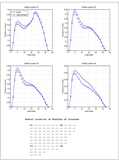
power perturbation. The error in the eigenvalue as a function of core power level

(43)

quantity for each power level and, hence, the accuracy in predicting this value can be

easily plotted as a function of core power level.

The comparison between the approximate and the exact change in k_eff as well as the error of the predicted change in k_eff are presented in the top and bottom plots of Figure 2.7, respectively. From these graphs, one can see that utilizing one iteration of the

first order Newton’s method, the change in the eigenvalue can be quite accurately

predicted. As expected, the error grows as the core being examined moves further away

from the reference 100% core power level. However, one should keep in mind that during

the course of Newton iterations, the fluctuations in core power will not likely come close

to that caused by the full range of core power level perturbation analyzed in this study.

This follows since the Jacobian matrix will be updated at each Newton iteration using the

latest iterative values. Figure 2.8 shows the comparisons of the approximate and exact

changes in the fast flux distribution for four radial locations (as shown in the core map

below the plots) when the core power level is perturbed by +10%, i.e. 110% core power

level. Although these plots represent an extreme perturbation in the core power, the

first-order approximation still predicts the axial power distribution reasonably well. Note that

slightly larger difference are observed in radial location “04”; however, recognizing the

size of the relative power, one can conclude that these larger differences are not too

important since the absolute differences are still relatively small. Based on these results, it

is safe to assume that the errors introduced by the first-order approximation are

insignificant.

The other thing learned from this study is that the Jacobian matrix is not singular.

The singularity of the Jacobian matrix becomes a concern since the block, defined as

, is singular when the value of is the true eigenvalue associated

with the generalized eigenvalue problem. This is indeed the case for our linearization error

study since we utilize the eigenvalue problem solution (at 100% core power level) as our

reference. However, in reality additional terms are added to to account for

cross-section changes due to fuel temperature changes. This follows since the cross-cross-section is a

J₁₁

M(ξ Ψ, ) λ– F(ξ Ψ, )

( ) λ

(44)

90 92 94 96 98 100 102 104 106 108 110 −400

−300 −200 −100 0 100 200 300 400 500

Core Power Level (%)

Change in k

eff

(pcm)

Exact Approximation

90 92 94 96 98 100 102 104 106 108 110

−5 0 5 10 15 20 25

Core Power Level (%)

Error in Delta k

eff

(45)

Radial Location of Bundles of Interest

01 02 --03 -- -- -- -- -- -- 04

--0 5 10 15 20 25 30

0 0.05 0.1 0.15 0.2 0.25 0.3 0.35 0.4

Axial Node

Relative Power

Radial Location 01

Exact Approximation

0 5 10 15 20 25 30

0 0.05 0.1 0.15 0.2 0.25 0.3 0.35 0.4 0.45

Radial Location 02

Axial Node

Relative Power

0 5 10 15 20 25 30

0 0.05 0.1 0.15 0.2 0.25 0.3 0.35 0.4 0.45

Radial Location 03

Axial Node

Relative Power

0 5 10 15 20 25 30

0 0.01 0.02 0.03 0.04 0.05 0.06

Radial Location 04

Axial Node

Relative Power

(46)

function of fuel temperature, which in turn is a function of power density, which in turn is

a function of flux, and we reduce the cross-section dependence to flux. These additional

terms when added to the block prevent this block from being singular.

2.4. Krylov Methods

Krylov methods are categorized as non-stationary iterative methods. For this

family of methods, information needed to advance from one iteration to the next keeps

changing. This means that when solving Eq. (2-11) for a fixed Newton iteration ,

allowing us to suppress the dependence and rewrite Eq. (2-11) as , we can

express the nthKrylov iteration of as

, (2-24)

where is the iterative matrix and is the remainder. When using unpreconditioned

Krylov methods, the nthiteration of is an element of

, (2-25)

which minimizes some norm measuring the distance between and the true solution,

. In Eq. (2-25), the initial residual ( ) is defined as

, (2-26)

where represents the initial guess and is the nth

Krylov subspace. How the coefficients (multipliers) of the bases for a particular Krylov

J₁₁

m

m JΘ = R

Θ

Θ( )n = GnΘ(n–1)+c

Gn c

Θ

Θ( )0 span r( )0 Jr( )0 … J

n–1 r( )0

, , ,

 

 

 

+

Θ( )n

Θ r( )0

r_{( )}₀ = R–JΘ_{( )}₀

Θ( )0 span r( )0 Jr( )0 … J

n–1 r( )0

, , ,

 

 

Implementation of a Newton-Krylov Iterative Method to Address Strong Non-Linear Feedback Effects in FORMOSA-B BWR Core Simulator

Abstract

Acknowledgment

Table of Contents

List of Tables

List of Figures

1. Introduction

2. Methodology