ABSTRACT
MARCEAU WEST, RACHEL ELIZABETH. Flexible Kernel Machine Methods for Complex Genomic Data. (Under the direction of Jung-Ying Tzeng and Wenbin Lu.)
Rare variant associations are essential to fully understanding and trying to effectively treat
complex diseases. Rare variants are often hypothesized to jointly explain much of the missing
heritability from common variant genome-wide association studies, and are believed to be more
likely than their common counterparts to have direct functional effect on disease etiology. However,
rare variant associations are still quite difficult to detect with existing statistical methodology,
especially when the question of interest goes beyond simple genetic main effect testing. Kernel
machine models provide a flexible framework to facilitate complex rare variant studies. We consider
three such interesting problems: (1) multi-factor analysis using multiple kernels to jointly model
different variable sets, testing for the effect of one set while adjusting for nuisance effects; (2)
cross-disorder gene variable selection, using kernels to leverage information on the co-occurrences of and
genetic correlations between diseases; and (3) rare variant prioritization using protein structure,
forming variant-level tests from local kernels that borrow information from variants that are nearby
on the protein tertiary space.
In project 1, we demonstrate use of a low-rank decomposition of the nuisance effect terms to
im-prove computational efficiency over traditional estimation (i.e., using an Expectation Maximization
algorithm or penalization). We extend this idea in project 2, showing how this decomposition can
be used to facilitate gene-level variable selection using group lasso when sample size and number
of variants is large. Further, in project 2 we demonstrate a significant power gain from borrowing
information from correlated diseases. In project 3, we continue looking at variable selection but try
to prioritize rare variants at the variant level and demonstrate how protein folding structure can be
incorporated into variant-level association testing to improve power and generate more biologically
interesting hypotheses.
binary, and survival traits. We further apply our methods to data from the Vitamin Intervention for
Stroke Prevention (VISP), CoLaus, and Action to Control Cardiovascular Risk in Diabetes (ACCORD)
© Copyright 2017 by Rachel Elizabeth Marceau West
Flexible Kernel Machine Methods for Complex Genomic Data
by
Rachel Elizabeth Marceau West
A dissertation submitted to the Graduate Faculty of North Carolina State University
in partial fulfillment of the requirements for the Degree of
Doctor of Philosophy
Statistics
Raleigh, North Carolina
2017
APPROVED BY:
Arnab Maity Eric Stone
Jung-Ying Tzeng
Co-chair of Advisory Committee
Wenbin Lu
DEDICATION
BIOGRAPHY
Rachel Elizabeth Marceau was raised equally in the Triad of North Carolina and in Nova Scotia,
Canada. She gained a love of statistics during her brief time at Southwest Guilford High School,
playing with M&M distributions in A.P. Statistics. After a short year studying astrophysics at the
University of Arizona, Rachel transferred to North Carolina State University to pursue her Bachelor’s
Degree in Statistics. During this time, she had the opportunity to take two genetics classes from Dr.
Ted Emigh, who piqued her curiosity in how statistics can be applied to help answer interesting
questions in the worlds of human genetics and population biology. She was able to further build
a passion for statistical genetics problems in the Computation for Undergraduates in Statistics
Program (CUSP) under the direction of Dr. David Reif and Dr. Alison Motsinger-Reif. In 2011, Rachel
graduated summa cum laude with a minor in mathematics. After a summer working with Dr. Spencer
Muse trying to quantify nonsynonymous mutation rates of mitochondrial DNA, she began her
graduate studies at NC State University, earning a Masters of Statistics in 2013 with a concentration
in statistical genetics. During this time, Rachel got married to her undergrad sweetheart Charlie
and gave birth to her wonderful daughter Clover. Rachel is set to obtain her Ph.D. in 2017 under
the direction of Dr. Jung-Ying Tzeng and Dr. Wenbin Lu, after which she hopes to continue working
towards improving our understanding of complex diseases through statistical analyses for many
ACKNOWLEDGEMENTS
I would like to start by thanking my incredible advisors Dr. Jung-Ying Tzeng and Dr. Wenbin Lu
for all of their support and guidance, as well as the rest of my committee, Dr. Eric Stone, Dr. Arnab
Maity, and Dr. Denis Fourches for all of their time, patience, knowledge, and thoughtful suggestions.
I would also like to thank my collaborators who provided access to the clinical trial data studied in
this paper, and who helped me to explore and better understand the complex genetic consequences
of our findings: Dr. Fang-Chi Hsu, Dr. Michèle Sale, Dr. Bradford Worrall, and Dr. Stephen Williams,
co-authors of the fastKM paper, and collaborators with the VISP c linical trial, and the ever-incredible
Dr. Mélaine Kuenemann, and Dr. Daniel Rotroff, from the ACCORD clinical trial project. I would also
like to thank Song et al. (2012) for access to thePLA2G7data, Dr. Fourches and Dr. Kuenemann for
use of their protein structure figures forPLA2G7andPCSK9, respectively, and Dr. Shannon Holloway
for her help in creating the fastKM R package.
I have been blessed to have many other wonderful mentors on my academic journey, including
Dr. Spencer Muse and Dr. Alison Motsinger-Reif, who have inspired and guided me since I was an
undergraduate student. I would also like to thank Dr. Joy Smith and Dr. Emily Griffith for guiding
me as a statistical consultant and as a person. I would also like to thank the countless professors
from NCSU who have helped my love of statistics grow.
Finally, I would like to thank my wonderful family and friends who have always supported me,
and my loving and patient husband, Charlie. Thank you for sticking with me through it all.
This dissertation was supported by the NIH training grant T32GM081057: Biostatistics Training
TABLE OF CONTENTS
LIST OF TABLES . . . vii
LIST OF FIGURES. . . ix
Chapter 1 Introduction. . . 1
1.1 Multi-Kernel Models . . . 3
1.2 Cross Disorder Analysis . . . 4
1.3 Rare Variant Prioritization via Protein Structure . . . 6
1.4 Summary of Dissertation . . . 7
Chapter 2 A Fast Multiple-Kernel Method with Applications to Detect Gene-Environment Interaction . . . 9
2.1 Abstract . . . 9
2.2 Key Words . . . 10
2.3 Introduction . . . 10
2.4 Materials and Methods . . . 13
2.4.1 The KM Model for G x E Interactions . . . 13
2.4.2 FastKM Test for G x E Interactions . . . 15
2.4.3 Extension to Survival Traits . . . 16
2.4.4 Implementation Detail . . . 17
2.4.5 Simulation Study . . . 18
2.4.6 Application to VISP Study . . . 19
2.5 Results . . . 21
2.5.1 Quantitative Traits . . . 21
2.5.2 Binary and Survival Traits . . . 26
2.5.3 VISP Study . . . 30
2.6 Discussion . . . 33
2.7 Acknowledgments . . . 35
2.8 Supplementary Materials . . . 35
2.8.1 Common Variants based Simulations . . . 35
Chapter 3 Cross Disorder Kernel Machine Modeling . . . 37
3.1 Abstract . . . 37
3.2 Introduction . . . 38
3.2.1 Motivation for Cross Disorder Analysis . . . 38
3.2.2 Current Methods . . . 39
3.2.3 Introduction to fastLasso . . . 47
3.3 Methods . . . 48
3.3.1 Kernel Evaluation . . . 49
3.3.2 Dimension Reduction . . . 50
3.3.3 fastLasso . . . 50
3.4 Simulation Study . . . 52
3.4.1 Data Generation . . . 52
3.4.2 fastLasso Simulation . . . 53
3.5 Results . . . 54
3.6 Discussion . . . 57
Chapter 4 Rare Variant Prioritization Using Structure-Supervised Kernel Association Tests. . . 59
4.1 Abstract . . . 59
4.2 Introduction . . . 60
4.3 Methods . . . 65
4.3.1 Structure-Supervised Kernel Machine Association Testing . . . 65
4.4 Simulation Study . . . 70
4.4.1 Simulation Set Up . . . 70
4.4.2 Simulation Study Results . . . 72
4.5 Application to ACCORD Study . . . 83
4.5.1 ACCORD Trial Background . . . 83
4.5.2 ACCORD Analysis . . . 84
4.5.3 ACCORD Results . . . 85
4.6 Discussion . . . 89
REFERENCES . . . 91
APPENDICES . . . .104
Appendix A Additional Information for Cross Disorder Kernel Machine Simulation 105 A.0.1 Case Control Sampling of Genotype Matrix for Binary Traits . . . 105
A.0.2 Cross Disorder and Single Disorder Tuning Parameter Summaries . . . 107
Appendix B Local Score Test Limiting Distribution . . . 108
Appendix C Additional Local Kernel Simulation Results . . . 113
C.0.1 Additional Simulation Results: Quantitative Traits Local Burden Kernel Test . . . 114
C.0.2 Additional Simulation Results: Binary Traits Local Burden Kernel Test . 116 C.0.3 Additional Simulation Results: Quantitative Traits Local Linear Kernel Test . . . 118
LIST OF TABLES
Table 2.1 Average run time in minutes (and corresponding standard error) for quan-titative traits when the G×E effect is zero with a sample size ofn =5, 000 individuals. . . 23 Table 2.2 Average run time in minutes (and corresponding standard error) for
quanti-tative traits when the G×E effect is nonzero with a sample size ofn=5, 000 individuals. . . 24 Table 2.3 P-values for the fastKM analyses of VISP study data, including (a) testing gene
×age interaction on post-methionine change in total Hcy, treating change as continuous, with a IBS kernel or polynomial kernel (d=2); (b) testing gene ×age interaction on post-methionine change in total Hcy, treating change as binary using the 90t h sample percentile as a cut off; (c) testing gene×
intervention interaction on time to recurrent stroke∗P-values that are<0.05. 32
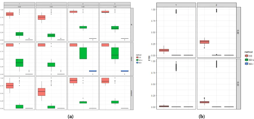
Table 3.1 Average true positive and false positive rates (and corresponding standard deviation) for cross disorder (CD), the union of single disorder (SD-U), and the intersection of single disorder (SD-I) continuous trait kernel machine model analyses over 100 simulations. Largest values within each category are in bold font. . . 56
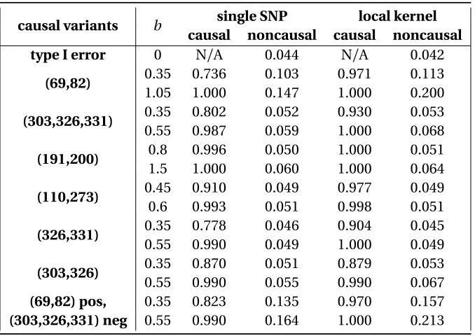
Table 4.1 Type I error and power for single-variant and local burden kernel tests for quantitative traits over various simulation scenarios usingPLA2G7protein tertiary structure . . . 74 Table 4.2 Type I error and power for single-variant and local burden kernel tests for
binary traits over various simulation scenarios usingPLA2G7protein tertiary structure . . . 75 Table 4.3 Type I error and power for single-variant and local linear kernel tests for
quantitative traits over various simulation scenarios usingPLA2G7protein tertiary structure . . . 78 Table 4.4 Type I error and power for single-variant and local linear kernel tests for
binary traits over various simulation scenarios usingPLA2G7protein tertiary structure . . . 79 Table 4.5 Scan statistic results for binary traits, summarized over 500 replications . . . . 82 Table 4.6 PCSK9rare variant single SNP and localized kernel test summary using PDB
entry 4K8R. Significant results are given in bold font. Q-values are calculated assumingπ0 =0 (e.g., Benjamini-Hochberg corrected values) due to low variant pool size. . . 86
Table C.1 Type I error and power for continuous trait local burden kernel test, weighted by minor allele frequency, withc = (0, 0.25, 0.5)over various causal variant scenarios usingPLA2G7protein tertiary structure . . . 114 Table C.2 Type I error and power for continuous trait local burden kernel test,
un-weighted, withc = (0, 0.25, 0.5)over various causal variant scenarios using PLA2G7protein tertiary structure . . . 115 Table C.3 Type I error and power for continuous trait local burden kernel test,
un-weighted, withc= (0, 0.1, 0.2, 0.3, 0.4, 0.5)over various causal variant scenarios usingPLA2G7protein tertiary structure . . . 115 Table C.4 Type I error and power for binary trait local burden test, weighted by minor
allele frequency, withc= (0, 0.25, 0.5)over various causal variant scenarios usingPLA2G7protein tertiary structure . . . 116 Table C.5 Type I error and power for binary trait local burden kernel test, unweighted,
withc = (0, 0.25, 0.5)over various causal variant scenarios usingPLA2G7 protein tertiary structure . . . 117 Table C.6 Type I error and power for binary trait local burden kernel test, unweighted,
withc = (0, 0.1, 0.2, 0.3, 0.4, 0.5)over various causal variant scenarios using PLA2G7protein tertiary structure . . . 117 Table C.7 Type I error and power for continuous trait local linear kernel test, weighted
by minor allele frequency, withc = (0, 0.25, 0.5)over various causal variant scenarios usingPLA2G7protein tertiary structure . . . 118 Table C.8 Type I error and power for continuous trait local linear kernel test, unweighted,
withc = (0, 0.25, 0.5)over various causal variant scenarios usingPLA2G7 protein tertiary structure . . . 119 Table C.9 Type I error and power for continuous trait local linear kernel test, unweighted,
withc = (0, 0.1, 0.2, 0.3, 0.4, 0.5)over various causal variant scenarios using PLA2G7protein tertiary structure . . . 119 Table C.10 Type I error and power for binary trait local linear kernel test, weighted by
mi-nor allele frequency, withc= (0, 0.25, 0.5)over various causal variant scenarios usingPLA2G7protein tertiary structure . . . 120 Table C.11 Type I error and power for binary trait local linear kernel test, unweighted,
withc = (0, 0.25, 0.5)over various causal variant scenarios usingPLA2G7 protein tertiary structure . . . 121 Table C.12 Type I error and power for binary trait local linear kernel test, unweighted,
withc = (0, 0.1, 0.2, 0.3, 0.4, 0.5)over various causal variant scenarios using PLA2G7protein tertiary structure . . . 121
LIST OF FIGURES
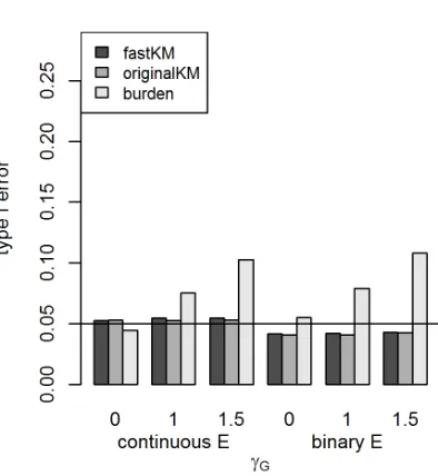
Figure 2.1 Type I error for fastKM, originalKM, and the weighted counting burden-based G×E test for quantitative traits withM =100 loci,n=5, 000 individuals, and varying main effect parameterγG. Models with a continuous
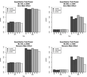
environ-mentalE covariate are on the left and those with a binary environmentalE covariate are on the right. The KM tests are based on the IBS kernel. . . 22 Figure 2.2 Power for fastKM, originalKM, and the weighted counting burden-based
G×E test for quantitative traits withM =100 loci andn=5, 000 individuals over varying interaction effect sizesγG E. The left panel shows the results of
no genetic main effect (i.e.,γG=0) and the right panels shows the results of
nonzero main effect (i.e.,γG=1). For each plot, continuousE covariates are
on the left and binaryE covariates are on the right. The KM tests are based on the IBS kernel. . . 23 Figure 2.3 Type I error for fastKM, originalKM, and the weighted counting
burden-based G×E test for quantitative traits with continuous environmentalE covariate and varying main effect parameterγG. The left panel shows the
results ofM=100 loci andn=5, 000 individuals. The right panel shows the results ofM =200 loci andn=1, 000 individuals. The KM tests are based on the IBS kernel and the polynomial kernels withd=2 and 3. . . 25 Figure 2.4 Power for fastKM, originalKM, and the weighted counting burden-based
G×E test for quantitative traits with continuousE covariate over varying main effect sizeγG (γG =0 for zero main effect, andγG =1 for nonzero main
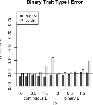
effect) and interaction effect sizeγG E. The left panel shows the results of M =100 loci andn=5, 000 individuals. The right panel shows the results of M =200 loci andn=1, 000 individuals. The KM tests are based on the IBS kernel and the polynomial kernels withd=2 and 3. . . 26 Figure 2.5 Type I error for fastKM and the weighted counting burden-based G×E test for
binary traits forM =100 loci,n=5, 000 individuals, and varying main effect parameterγG. Models whereE is generated from a Gaussian distribution
are displayed on the left, and those whereE is from a Bernoulli distribution are on the right. The KM tests are based on the IBS kernel. . . 27 Figure 2.6 Type I error for survival traits for fastKM and the weighted counting
Figure 2.7 Power for fastKM and the weighted counting burden-based G×E test for binary traits withM =100 loci andn=5, 000 individuals over varying inter-action effect sizesγG E. The left panel shows the results of no genetic main
effect (i.e.,γG =0) and the right panels shows the results of nonzero main
effect (i.e.,γG =1). For each plot, continuousE covariates are on the left and
binaryE covariates are on the right. The KM tests are based on the IBS kernel. 29 Figure 2.8 Power for fastKM and the weighted counting burden-based G×E test for
survival traits withM =100 loci andn=5, 000 individuals for varying in-teraction parameterγG E over two censoring proportions (c=15% and 40%).
The left panel shows the results of no genetic main effect (i.e.,γG =0) and
the right panels shows the results of nonzero main effect (i.e.,γG =1). For
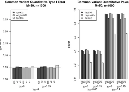
each plot, continuousE covariates are on the left and binaryE covariates are on the right. The KM tests are based on the IBS kernel. . . 29 Figure 2.9 Type I error (left panel) and power (right panel) for fastKM, originalKM, and
the weighted counting burden-based G×E test for common variants with continuous E covariate over varying main effect sizeγG and interaction
effect sizeγG E. The KM tests are based on the IBS kernel and the polynomial
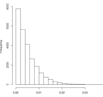
kernels withd=2 andd=3, all with 95% kPCA. . . 36 Figure 3.1 Histogram of the non-zero coefficients from the null model fastLasso fit . . . 54 Figure 3.2 True positive and false positive rates for cross disorder (CD), the union of
sin-gle disorder (SD-U), and the intersection of sinsin-gle disorder (SD-I) continuous trait kernel machine model analyses over 100 simulations . . . 57
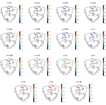
Figure 4.1 PLA2G7(a) rare variants location on the protein tertiary structure, and (b) corresponding Euclidean distance-based clustering of variants. Protein ter-tiary structure published with permission from Dr. Fourches. . . 71 Figure 4.2 Amount of borrowing from neighboring variants forPLA2G7variant 110 for
different values ofc. . . 73 Figure 4.3 Variant correlation forPLA2G7SNVs . . . 76 Figure 4.4 Summary of proportion of times a givenc value was chosen as optimal for
the local burden kernel test for causal and noncausal variants . . . 76 Figure 4.5 Variant selection probabilities for single variant and local burden kernel
tests, separated by noncausal variants (effective type I error), and causal variants (effective power) . . . 77 Figure 4.6 Summary of proportion of times a givenc value was chosen as optimal for
the local linear kernel test for causal and noncausal variants . . . 80 Figure 4.7 Variant selection probabilities for single variant and local linear kernel tests,
separated by noncausal variants (effective type I error), and causal variants (effective power) . . . 80 Figure 4.8 Variant borrowing for the best scalec for local kernel tests of association
Chapter 1
Introduction
A major goal in statistical genetics is to facilitate genetic association studies involving complex
genomic data - finding links between genes and phenotypes to help us better understand the etiology
of complex diseases and thus how to better classify and treat them. Genome-wide association studies,
or GWAS, have been used quite extensively in the past to look for associations between common
genetic variants and disease phenotypes. However, these simple analyses leave a high proportion
of heritability unexplained (Eichler et al., 2010, Manolio et al., 2009). Increasing attention is being
placed on rare variants which occur infrequently (e.g., with a minor allele frequency, or MAF of
less than 1%) in the human population, with researchers hypothesizing that combined effects
from many of these rare variants within different genes may be able to explain a lot of this missing
heritability (Bodmer and Bonilla, 2008, Eichler et al., 2010, Manolio et al., 2009, Morris and Zeggini,
2010). Improving genotyping technology, such as the introduction of Next Generation Sequencing
(NGS) technology, which facilitates sequencing of billions of short reads relatively inexpensively
(Lee et al., 2014), has improved our access to rare variant data, further motivating the shift in focus
to studying less frequent variants.
Rare variants, however, tend to be quite difficult to detect individually, requiring much larger
challenge, especially when considering more complex genetic data. Two main classes of methods
have been proposed to increase our power to detect rare variant associations. The first are
burden-based methods (e.g., Li and Leal (2008), Madsen and Browning (2009), Morris and Zeggini (2010),
Price et al. (2010)), which aggregate information across a set of variants using a weighted sum of
effects. These models are quite simple to fit, but lose power from collapsing over noise variants,
and possibly over variants with opposite effects. The second are similarity-based approaches, using
the (statistically and intuitively) related mixed effects models (e.g., Goeman et al. (2004), Lin et al.
(2013)), similarity regressions (e.g., Tzeng et al. (2014, 2009, 2011), Wang et al. (2014), Zhao et al.
(2015)), and kernel machine models (e.g., Kwee et al. (2008), Lin et al. (2011), Liu et al. (2008, 2007),
Wu et al. (2010, 2011, 2013)). These approaches aggregate information from multiple variants in a
flexible manner, modeling the genetic similarity between pairs of individuals in variance/covariance
of genetic random effect terms, similarity matrices, or kernel matrices, respectively.
We focus our attention on the robust kernel machine (KM) models. Kernel machine models
allow for incorporation of complex genomic relationships, easily modeling nonlinear/non-additive
epistatic effects. The framework can be be applied to multiple trait types, such as continuous, binary,
and survival traits, and can provide efficient dimension reduction to facilitate analysis of large
sample size data required for rare variant analysis.
In this dissertation, we show how the kernel machine framework can be used to approach three
important topics within rare variant genetic association testing:
1. Multi-kernel analyses, testing for association while accounting for nuisance effects, (e.g.
ac-counting for genetic main effect terms when testing for gene-environment interaction, or
testing for genetic main effect when accounting for population substructure),
2. Cross-disorder analyses, using unified information to better understand pleiotropy and
dis-cover genes associated with at least one trait, and
1.1
Multi-Kernel Models
Kernel machine models with multiple kernels can be useful for incorporating multiple random
effects terms into a rare variant genetic association analysis, e.g., testing for gene-environment
(GxE) (Lin et al., 2013, Tzeng et al., 2011, Wang et al., 2015d, Zhao et al., 2015) or gene-gene (GxG)
(Larson and Schaid, 2013, Wang et al., 2014) interaction while accounting for genetic main effect,
testing for genetic main effect while accounting for population substructure, or even testing for copy
number variant (CNV) dosage while accounting for CNV length (Tzeng et al., 2015). With multiple
effect terms, model misspecification is even more of a problem than with single variant-set genetic
main effect models, so the robustness of KM models (e.g., over burden models) becomes even more
important (Wang et al., 2015d).
The multi-kernel KM model is powerful, robust, and flexible but requires estimation of
nui-sance effects in order to perform valid score tests. Estimation of these nuinui-sance effects can be
very demanding due to their high dimensional nature, with dimension equal to the sample size.
Existing approaches to estimating nuisance effects typically use penalization or an
Expectation-Maximization (EM) algorithm. Penalization approaches (e.g., Lin et al. (2013)) use regularization
to impose more sparse solutions, leading to easier estimation. EM algorithm-based approaches
(e.g. Tzeng et al. (2011), Wang et al. (2014, 2015d), Zhao et al. (2015)) treat the nuisance variable
as a random effect and aim to estimate the corresponding variance component. Both types of
ap-proaches are quite computationally demanding due to tuning or to multiple large matrix inversions,
respectively, and do not straightforwardly extend to other trait types. They are especially more
difficult to use for rare variant analyses, where in general larger sample sizes are required to obtain
sufficient signal.
Kernel matrices in rare variant genetic association studies, however, typically have the property
of being low rank, with rank often much less than the minimum of the sample size and number
variants within a set may be quite low for rare mutations. Therefore, a low rank approximation
of the nuisance kernel can be used in place of the kernel itself, allowing for the nuisance effects
to be estimated as a low dimensional fixed effects term for which penalization is not necessary.
The “fastKM” method does this low rank approximation to help make multi-kernel analyses more
manageable, bending the problem down to an effective single kernel model which can be fit using
existing software (e.g., SKAT (Wu et al., 2011)), while maintaining proper type I error and power as
can be found using the much slower EM-based and penalization-based approaches.
1.2
Cross Disorder Analysis
KM models can also be useful for rare variant cross-disorder analysis. This is an important topic as
we can use information on correlated traits to increase our power to detect genetic associations
and yield more biologically accurate understanding of the disorders considered, helping us to
understand pleiotropy, or the effect a gene has on a set of traits (Casale et al., 2015, Korte et al., 2012,
Li et al., 2014, Zhou and Stephens, 2014). With rare variants having lower minor allele frequency,
appearing infrequently in smaller populations, with weaker effects, having effectively increased our
sample size can help increase signal (Li et al., 2014, Maier et al., 2015).
Currently, three main approaches exist to analyze multi-trait data: meta-analysis and combined
tests, dimension reduction, and multi-trait regression (Galesloot et al., 2014, Yang and Wang, 2012).
Meta analyses, including the work of Andreassen et al. (2013), Bolormaa et al. (2014), Yang et al.
(2010) and Van der Sluis et al. (2013), combine summary statistics (e.g., test statistics or p-values)
from single trait genome-wise association studies (GWAS). Because they work with summary statistic
data, they can combine data from non-overlapping individuals – even from published results – and
can analyze traits that do not follow the same distribution, e.g. continuous and dichotomous traits
simultaneously (Bolormaa et al., 2014, Van der Sluis et al., 2013, Yang et al., 2010). They easily scale up
(Bolormaa et al., 2014, Van der Sluis et al., 2013, Yang et al., 2010). However, they lose power due to
high multiple testing burden and by not incorporating coheritability and comorbidity information
(Wang et al., 2015b).
Dimension reduction methods use principal component analysis (PCA) (e.g., Aschard et al.
(2014), Klei et al. (2008)) and canonical correlation analysis (e.g., Ferreira and Purcell (2008)) to create
a low-rank summary of the multiple phenotypes, trying to create a new response that explains the
highest proportion of variability in phenotype or heritabiity (or covariability between phenotype and
genotype). These approaches directly incorporate the correlations between phenotypes (Aschard
et al., 2014), but are not easily interpretable, looking at linear combinations of traits rather than the
actual traits. They also tend to focus on Gaussian distributed traits.
The last class, multi-trait regression often uses a random effects approach to directly model
variance/covariance of genotypes between and within traits. Many multivariate linear mixed effects
models (mLMMs) have been proposed to estimate coheritabilty and genetic correlation as a
surro-gate for pleitropy (e.g., Korte et al. (2012), Lee et al. (2012b), Loh et al. (2015), Vattikuti et al. (2012)),
or to predict genetic risk (e.g., Maier et al. (2015)). They have also been used to test for genetic
association (e.g., Casale et al. (2015), Zhou and Stephens (2014)). These models are interpretable
and successfully borrow information between traits, but assume normally distributed, or linearized,
phenotype data. Other multi-trait regression models have also been proposed, e.g., looking at a
functional linear regression for continuous gene-location incorporation (Wang et al., 2015b), using
bivariate ridge regression for whole-genome genetic risk prediction (Li et al., 2014), or, finally, using
similarity or kernel frameworks (Broadaway et al., 2016, Maity et al., 2012, Wei and Lu, 2015). These
approaches provide additional flexibility, looking at how trait similarity relates to genotype similarity,
but doesn’t allow us to pinpoint genes with rare variants that are significantly associated with at
least one disorder.
As in Maity et al. (2012), the kernel machine framework can be used to model complex
with group lasso, kernels can be very useful for performing variable selection to detect which
vari-ants are likely associated with at least one disorder, combining information in a direct but flexible
manner. Using a fastKM approximation makes this approach feasible and efficient.
1.3
Rare Variant Prioritization via Protein Structure
Since rare variants can be so difficult to identify individually, rare variant association tests usually
require borrowing of signal - from other rare variants, or from additional genetic annotation
informa-tion. When causal variant prioritization is of interest, however, straight aggregation of information
over all rare variants within a variant set is not helpful, as it does not allow you to detect where the
signal is likely coming from. Two main classes of genetic variant localization (prioritization) exist in
the literature: penalization and most promising subset approaches.
Penalization methods use regularization to incorporate information from multiple genetic
vari-ants without forcing collapsing, shrinking estimates of noncausal loci or groups of loci. Examples
include the work of Larson and Schaid (2014), Xu et al. (2012), and Zhou et al. (2011, 2010),
exam-ining the effects of group and combined penalties on power to detect likely causal rare variants.
These methods are powerful but do not perform explicit association testing, and require sufficient
sequencing information.
Most promising subset methodology, on the other hand, looks at clustering variants and trying
to identify which clusters are most likely to be causal. They are based on the assumption that causal
variants are likely to be close together in some dimension, be it on the 2 dimensional sequence, 3
dimensional structure, or functional domain (Fier et al., 2012, Ionita-Laza et al., 2012, Larson and
Schaid, 2014, Yue et al., 2010). Some (e.g., Ionita-Laza et al. (2012), Kulldorff (1997)) create windows of
variants along DNA sequence, assuming causal variants have the same effect on the trait of interest,
with decreasing power for decreasing window and gene size, and decreasing variability within a
(2010)) have used kernel approaches to perform spatial clustering of variants, but focus on DNA
sequence location to cluster variants. They also do not prioritize variants or calculate variant-level
significance.
The kernel machine framework can be used here as well to incorporate biostructural information,
e.g. location in the protein tertiary folding space, to perform local variant-level tests while still
borrowing information from neighboring variants. Local kernels can be defined for each variant
to determine the genetic similarity between individuals for a variant and those nearby on the
3-dimensional protein space, weighting on Euclidean distance from each variant, providing a local
kernel machine framework. This is motivated by the idea that variants nearby on the protein tertiary
space are more likely to behave similarly, e.g. due to binding domains or hydrophobic/hydrophilic
nature of a region (Song et al., 2012).
1.4
Summary of Dissertation
The rest of the dissertation proceeds as follows: in chapter 2, we propose the fast kernel machine
“fastKM” method for approximating nuisance effect kernels with low-dimensional fixed effects terms,
showing how it can be used to facilitate analysis of multiple kernel models (e.g., GxE analysis) in an
efficient manner. We demonstrate its utility in a simulation study, showing it is as powerful as an
EM-based approach for estimating nuisance variance components, but much faster for continuous and
binary traits, and makes the analysis of survival traits feasible. We further apply the fastKM method
to the Vitamin Intervention for Stoke Prevention clinical trial to understand the effects of
gene-by-vitamin regimen and gene-by-patient age on recurrent stroke risk and change in homocysteine
level, respectively. Chapter 2 has been previously published in Genetic Epidemiology (Marceau
et al., 2015).
In chapter 3, we propose the related “fastLasso” method for performing gene selection in
to provide an efficient way to analyze genetic effects on multiple traits simultaneously, improving
our power to detect genes associated with at least one disorder and flexibility to include different
subjects for binary and continuous traits. We perform a simulation study to compare this
cross-disorder analysis with the union of single cross-disorder analyses, showing it increases the true positive
rate while keeping a similar average false positive rate.
Finally, in chapter 4 we further examine the notion of prioritization of causal variants. We define
a framework for incorporating protein tertiary structure into a kernel machine modeling approach to
create powerful local (variant-level) kernel tests for rare variant association. We perform a simulation
study, showing how our method is more powerful than single variant score tests and the
sequence-based scan statistic, while maintaining a reasonable type I error for binary and continuous traits. We
further apply our method to the Action to Control Cardiovascular Risk in Diabetes (ACCORD) clinical
trial, prioritizing rare variants associated with lowering low-dentisty lipoprotein (LDL), finding three
new promising variants which appear to fall within or near to thePCSK9-LDLRprotein-binding
Chapter 2
A Fast Multiple-Kernel Method with
Applications to Detect
Gene-Environment Interaction
Rachel Marceau, Wenbin Lu, Shannon Holloway, Michèle M. Sale, Bradford B. Worrall, Stephen
R. Williams, Fang-Chi Hsu, Jung-Ying Tzeng
*previously published inGenetic Epidemiology(Marceau et al., 2015)
2.1
Abstract
Kernel machine (KM) models are a powerful tool for exploring associations between sets of genetic
variants and complex traits. Although most KM methods use a single kernel function to assess the
marginal effect of a variable set, KM analyses involving multiple kernels have become increasingly
popular. Multikernel analysis allows researchers to study more complex problems, such as assessing
gene-gene or gene-environment interactions, incorporating variance-component based methods
effects of a variable set adjusting for other variable sets. The KM framework is robust, powerful,
and provides efficient dimension reduction for multifactor analyses, but requires the estimation of
high dimensional nuisance parameters. Traditional estimation techniques, including regularization
and the “expectation maximization (EM)” algorithm, have a large computational cost and are not
scalable to large sample sizes needed for rare variant analysis. Therefore, under the context of
gene-environment interaction, we propose a computationally efficient and statistically rigorous “fastKM"
algorithm for multikernel analysis that is based on a low-rank approximation to the nuisance effect
kernel matrices. Our algorithm is applicable to various trait types (e.g., continuous, binary, and
survival traits) and can be implemented using any existing single-kernel analysis software. Through
extensive simulation studies, we show that our algorithm has similar performance to an EM-based
KM approach for quantitative traits while running much faster. We also apply our method to the
Vitamin Intervention for Stroke Prevention (VISP) clinical trial, examining gene-by-vitamin effects
on recurrent stroke risk and gene-by-age effects on change in homocysteine level.
2.2
Key Words
multiple-kernel analysis; kernel machine regression; exon level association test; gene-environment
interaction; gene-gene interactions
2.3
Introduction
Kernel machine (KM) based approaches (Kwee et al., 2008, Lin et al., 2011, Liu et al., 2008, 2007, Wu
et al., 2010, 2011) provide a powerful and popular strategy for evaluating associations between a set
of genetic variants and complex traits of various types. The KM method uses a kernel function to
quantify the pairwise genetic similarity for individuals based on multiple genetic variants; it then
assesses the gene-trait association by examining if the genetic similarity of a pair of individuals
methods, for example, variance component tests (Goeman et al., 2004, Lin et al., 2013) and similarity
regressions (Tzeng et al., 2014, 2009, 2011, Wang et al., 2014, Zhao et al., 2015), are closely related to
KM tests under a random effects model. Therefore, although this paper primarily focuses on KM
methods, the proposed approach and discussions are applicable to other variance component and
similarity-based tests.
While the popular KM methods, for example, the Sequence Kernel Association Test (SKAT)
(Wu et al., 2011), focus on single-kernel analysis (i.e., using one kernel function to model a single
variable set), analyses involving multiple kernels (i.e., using separate kernels to simultaneously
model multiple variable sets) are also frequently encountered in genomic research. Multikernel
approaches include tests for gene-environment (G×E) interactions (Lin et al., 2013, Tzeng et al.,
2011, Wang et al., 2015d, Zhao et al., 2015), tests for gene-gene interactions (Larson and Schaid,
2013, Wang et al., 2014), conditional tests for evaluating the effect of a single variable set adjusting
for other variable sets (Pang et al., 2014, Wang et al., 2015c,d), and SKAT analysis coupled with a
variance component method (Kang et al., 2010) to account for population substructure. The number
of explanatory variables in these analyses is much higher than in a single marker-set analysis. In
these situations, KM offers efficient dimension reduction and yield higher power to evaluate the
effects of interest compared to other alternatives, such as burden-based methods (e.g., Madsen and
Browning (2009), Price et al. (2010)). In addition, KM methods can model nonlinear/non-additive
effects, accommodate variables with different direction and magnitude of effects, and are more
robust than burden-based methods because they impose fewer assumptions on the underlying
effects. The latter is particularly important in multikernel analysis — for example, a KM G×E test is
more robust against misspecification of the main effects of G and E than the burden-based G×E test
(Wang et al., 2015d).
However, the merits of KM approaches come with high computational cost for multikernel
analyses, which substantially limits their practical utility. In a multikernel model, each effect is
of individuals). Computing the test statistic to evaluate the effect of interest in a multikernel analysis
requires estimation of at least one set ofn-dimensional nuisance parameters. For example,
per-forming a KM G×E test, even under the null hypothesis of no G×E effects, requires the estimation
of nuisance genetic main effects. Current attempts to overcome the dimensionality challenges
include treating then-dimensional parameters as random and using the EM algorithm to estimate
its variance component (Tzeng et al., 2011, Wang et al., 2014, 2015d, Zhao et al., 2015), or
impos-ing penalization on these parameters (Lin et al., 2013). While both techniques have proven to be
valid, the estimation procedures are usually phenotype-specific (e.g., the algorithms developed
for quantitative traits cannot be applied to binary or survival traits) and computationally intensive
(e.g., requiring the inversion of an-dimensional matrix at each iteration of the EM algorithm or the
tuning of a regularization parameter), making them not scalable to the large samples considered in
rare variant studies.
Using KM tests for G×E interactions as an example, we illustrate our solution to resolve these
computational challenges: a computationally efficient and statistically rigorous algorithm for
per-forming KM tests in multikernel analyses. Our algorithm is motivated by the fact that then×nkernel
matrix is often not full rank — its rank is generally much less than the minimum of the number of
individuals and the number of variables (e.g., SNPs) in a variable set. Thus, by decomposing the
kernel matrices of nuisance effects, we can reduce the dimensionality to a manageable size so that
a random-effect treatment or penalization is not necessary, and consequently a fixed effect null
model can be fit to estimate nuisance parameters. The proposed method is fast, scalable to largern,
and applicable to a variety of trait types; most importantly, it can be implemented using any existing
software for single KM analysis. For example, our algorithm would allow one to perform a KM G×E
test using the existing software for main effect KM tests, such as SKAT.
We explore the performance of our method through an in-depth simulation study for
quantita-tive, binary, and survival traits. We also apply our method to the Vitamin Intervention for Stroke
the homocysteine pathway, we examine the gene-by-vitamin effects on recurrent stroke risk (Hsu
et al., 2011, Tzeng et al., 2014) and gene-by-age effects on change in homocysteine level (Tzeng et al.,
2011). In such, we are able to see the true flexibility and unifying features of our method, in its ability
to perform multikernel analysis for different trait types in a computationally efficient manner.
2.4
Materials and Methods
2.4.1 The KM Model for G x E Interactions
Consider a study withnindividuals. For individuali,i =1, ...,n, letYi denote the phenotype of
interest andGi= (gi1, ....,gi M)T denote the genetic markers. For now we assume an additive genetic
effect wheregi mis the count of minor alleles that individuali has at markerm,m=1, ...,M, though
it is straightforward to extend this to recessive or dominant modes of inheritance. In addition, let
Xi= (1,Xi1, ...,Xi q)T denote the baseline covariates that have no interaction with genetic markers
andEithe covariate interacting with genetic markers. For simplicity, we assume thatEiis a scalar.
We consider a generalized linear model forYi
g(µi) =XiTβX +EiβE+hG(Gi) +hG E(Gi,Ei), (2.1)
whereµi=E(Yi|Xi,Ei,Gi),g(µi)is a canonical link function, for example,g(µi) =µifor quantitative
traits andg(µi) =logit(µi) =log
µ
i
1−µi
for binary traits,hG(·)andhG E(·)are two nonparametric smooth functions representing the main effect of genetic markers (i.e., G effect) and interaction
effect between theE covariate and genetic markers (i.e., G×E effect). Model (1) can also be expressed
in matrix notation as
g(µ) =XβX +EβE+hG(G) +hG E(G,E), (2.2)
andhG(G) = (hG(G1), ...,hG(Gn))T.
Under this model, we can test for G×E interaction using the null hypothesisH0:hG E(·) =0. Since hG(·)andhG E(·)are smooth functions that lie in a Hilbert space, by the representer theorem we can writehG(G)andhG E(G,E)in dual form expressions (Kimeldorf and Wahba, 1971):hG(G) =KGαG
andhG E(G,E) =KG EαG E, whereKG={KG(Gi,Gj): 1≤i,j≤n}is ann×nkernel matrix for the G
effect,KG E ={KG E({Gi,Ei},{Gj,Ej}): 1≤i,j≤n}is ann×nkernel matrix for the G×E effect, and
αG andαG E aren×1 vectors of unknown parameters. One commonly adopted kernel function for
theG main effect is the weighted identity by state (IBS) kernel (Kwee et al., 2008, Wu et al., 2010),
that is,KGI B S(Gi,Gj) =
PM
m=1wm{2I(gi m=gj m)+I(|gi m−gj m|=1)}
PM m=1wm
. The IBS kernel quantifies genetic similarity
using the weighted average number of alleles for which two individuals have in common in the
marker set. The weightswm0s are prespecified to upweight or downweight a variant based on certain
features. For example, one can weight against the minor allele frequency of markerm so as to
upweight similarities that are contributed by rare variants. Given the genetic main effect kernel
KG, one possible way to construct the interaction kernelKG E is to take the element-wise product
of the genetic main effect kernel and the environmental kernelKE, as described in Larson and
Schaid (2013) and Wang et al. (2015d). When the environmental covariate is a scalar, this simplifies
toKG E =DEKGDE, whereDE is a diagonal matrix with elementsE (Tzeng et al., 2011). However,
caution must be taken when using this direct product kernel to avoid duplicating the main effect
terms in the GxE kernel (Wang et al., 2015d).
The smooth functionshG E(G,E)can be viewed as random effects (Liu et al., 2008, 2007) and modeled through a multivariate normal distribution with mean zero and variance-covariance
τG EKG E, that is,hG E(G,E)∼N(0,τG EKG E). This is equivalent toαG E ∼N(0,τG EKG E−1)because hG E(G,E) =KG EαG E. Using this representation, testingH0:hG E(.) =0 is equivalent to testing the
null hypothesisH0:τG E =0 via a variance component score test (Liu et al., 2008, 2007).
Lin (1997) showed that the variance component score test is locally most powerful for testing
generalized linear model. For interaction tests however, fitting the null model requires estimation
of the nonparametric functionhG(·). There are two main approaches for fitting the null model: the first strategy treatshG(G)as random effects following a multivariate normal distribution with mean zero and variance-covarianceτGKG, and uses an EM algorithm to estimate the nuisance
variance componentτG (e.g., Tzeng et al. (2011), Wang et al. (2014, 2015d), Zhao et al. (2015)). The
second strategy uses penalization techniques, such as ridge regression, to estimate then×1 vector
of parametersαG (e.g., Lin et al. (2013)). Both strategies, however, are difficult computationally. The
random effect approach is time consuming due to inverting ann×nmatrix at each iteration of the
EM algorithm, and has difficulties with estimation on the boundary of the parameter space. On the
other hand, penalization methods require selection of a proper tuning parameter.
2.4.2 FastKM Test for G x E Interactions
We propose to take advantage of the low-rank structure of the kernel matrixKG to enhance
com-putational efficiency. Clearly, the weighted IBS kernel matrix is almost never full rank–typically,
r a n k(KG)<<m i n(n,M)(i.e., less than the number of individuals and the number of markers of interest). SinceKG is a symmetric matrix, it can be decomposed using eigendecomposition as
KG=QΛQT, whereQis the matrix of eigenvectors ofKG andΛis a diagonal matrix of eigenvalues
ofKG. Removing the near-zero eigenvalues or taking only the leading eigenvalues that capture a
high percentage of the total variation results in a low-rank decompositionKG =Zn×rZrT×n, where r <<nis the number of positive eigenvalues kept. The null model, then, reduces to the form
g(µ) =XβX +EβE+Z ZTαG¬XβX +EβE+Zγ. (2.3)
whereγ=ZTαG. Model (2.3), referred to as the fastKM null model, is a standard GLM with low
dimensional parameters. The fastKM null model can be rewritten in terms of an augmented design
Aθ; the parameterθcan be directly estimated by the maximum likelihood estimation using standard
software. In the same spirit, we can rewrite Model (2.2) and obtain the following fastKM model:
g(µ) =XβX+EβE+Zγ+hG E(G,E). We then construct the score test statistic forH0:τG E =0 as Un=n−1(ε1ˆ , ... ˆεn)KG E(ε1ˆ , ... ˆεn)T, where ˆθis the maximum likelihood estimator ofθunder the null
and ˆεi=Yi−g−1(ATiθˆ)(i=1,· · ·,n) are fitted residuals.
Note that our score test statistic shares the same form of the KM score test statistic for genetic
main effects (except thatKG E is involved instead ofKG). Therefore, the KM G×E test can be
con-ducted using any existing testing software for genetic main effects, such as SKAT (Wu et al., 2011),
providing the augmented design matrixAand the G×E kernelKG E as input. Moreover, as with main
effect KM tests, the limiting distribution of the fastKM test statistic under the null can also be
repre-sented asPdi=1λiχ1,2i, whereχ1,2i(i=1,· · ·,d) are independent Chi-squared random variables with
one degree of freedom and weightsλi’s are the positive eigenvalues of a nonnegative definite matrix
Σ. Here matrixΣis the variance-covariance matrix of the limiting distribution ofn−1/2Pn
i=1εˆiZG E,i, whereZG E,i is thei-th row of matrixZG E withZG EZG ET =KG E (Lin, 1997, Zhang and Lin, 2003).
The associatedP-value can be calculated using moment matching method (Duchesne and Lafaye
De Micheaux, 2010), the Davies method (Davies, 1980), or empirically using resampling techniques.
For a resampling method, one can generate many sets of independent Chi-squared random variables
with one degree of freedom and calculateUn,b =
Pd
i=1λˆiχ1,2i,b=1, ...,B, where ˆλiis a consistent
estimator ofλi. Then the estimatedP-value isB−1
PB
b=1I(Un<Un,b).
2.4.3 Extension to Survival Traits
As of yet, no methods have been developed for testing marker-set G×E effects for survival traits.
Our fastKM method, however, can be naturally extended to include survival traits. For individuali,
in Tzeng et al. (2014). Under the null, we fit the proportional hazards model with the augmented
covariatesAias defined previously. Let ˆθdenote the maximum partial likelihood estimator ofθand
ˆ
Λ(·)denote the Breslow estimator of the baseline cumulative hazard function. Our proposed test statistic for the null hypothesisH0:hG E(.) =0 is given byUn=n−1(ε1ˆ , ... ˆεn)KG E(ε1ˆ , ... ˆεn)T, where
ˆ
εi=δi−Λˆ(T˜i)exp(ATi θˆ)(i=1,· · ·,n) is a martingale residual. The fastKM test statistic again shares
the same form as the score test statistic for the genetic main effect tests discussed in Lin et al. (2011)
and Tzeng et al. (2014), with our augmented design matrixAas the covariate design matrix and
G×E kernelKG E as the kernel matrix. Consequently, the fastKM test statistic and itsP-value can be
obtained by using the existing software for KM main-effect tests with survival traits (e.g., Lin et al.
(2011), Tzeng et al. (2014)).
2.4.4 Implementation Detail
In practice, the low rank decomposition may contain several near-zero eigenvalues, which would
result in theZ matrix (and hence also the augmented design matrixA) containing multiple
near-zero columns and lead to unstable parameter estimation. We suggest performing kernel principal
component analysis (kPCA) to further reduce dimensionality and improve stability (Cai et al., 2011,
Schölkopf et al., 1998). In practice, choosing to keep the top eigenvalues that collectively explain
p=95% or 99% of the total variability can give good empirical results, especially for continuous traits. However, when the variants of interest are rare and there are many near-zero eigenvalues, a
smallerp may be necessary for achieving estimation stability with binary and survival traits. In our
numerical studies (simulation and real data analysis), we identify a suitablep% by starting with a
high percentage (e.g., 99%) and then gradually reducingpuntil the null model fits reasonably well
(e.g., no warning messages in the GLM fits or no extremely large coefficients). This is also the rule
2.4.5 Simulation Study
2.4.5.1 Data Generation
We generated a set of 10,000 haplotypes using the COSI software of Schaffner et al. (2005) with a
coalescent model mimicking the linkage disequilibrium and population history of the European
population. We then formed a marker-set ofM rare (minor allele frequency<0.05) loci, of which
the first 40 were considered causal. We generated a sample ofnindividual genotypes by randomly
sampling two haplotypes with replacement. We setM =100 loci andn=5000 individuals. We also consideredM =200 andn=1000 in a subset of scenarios to investigate the impact ofM andn on the performance of fastKM. We considered a single environmental covariateE that is either
continuous (generated from a Normal(0,1) distribution) or binary (generated from a Bernoulli(0.5)
distribution). We assumed no confounding covariates in the simulations.
We evaluate the performance of the fastKM G×E tests using data generated from a fixed effect
model, where the genetic main and interaction effects depend on mutational burden.
Specifi-cally, given each individual’s environmental covariate and genotypes, defineη(Ei,Gi) =γ0+γEEi+
γG
PMc
m=1gi m+γG EEi(
PMc
m=1gi m), whereMc =40 represents the number of causal variants. We considered three types of traits: quantitative, binary, and survival. Quantitative responses were
generated from the modelYi =η(Ei,Gi) +εwhereε∼N(0, 1). Binary responses were generated
in a case-control framework from a Bernoulli distribution withP(Yi=1|Ei,Gi) = e
η(Ei,Gi)
1+eη(Ei,Gi). Finally, survival traits were generated from a Cox proportional hazards model: log(Ti) =−η(Ei,Gi) +ε∗i,
2.4.5.2 Examining Power and Type I Error of FastKM
In each simulation scenario, we perform 2000 replicates for type I error analysis and 1000 replicates
for power analysis. We compared our fastKM G×E test to the burden-based G×E test. For quantitative
traits, we also compare with the traditional EM-based KM G×E test (referred to as “originalKM”).
We calculated the IBS kernel forKG as described in Tzeng et al. (2011) and set the variant-specific
weight aswm = (1−qm)24(Wu et al., 2011). For certain settings under quantitative traits, we also
calculated the polynomial kernel (i.e.,KGp o l y= (1+GiTGj)d) withd=2 andd =3.
After performing the eigenvalue decomposition of KG, we rounded those eigenvalues with
magnitude<10−10to zero, and kept the top eigenvalues to explainp% of the variability (p% kPCA);
the value ofp is chosen to retain the maximum amount of variation while still yielding stable GLM
estimates.
For the fastKM algorithm, we fit the fastKM null model for each trait with linear predictor
η(A) =γ0+γAAwhereAis the augmented design matrix composed of a standardized covariate and the reduced Z matrix.P-values were calculated using the Davies method (Davies, 1980) as
implemented in Duchesne and Lafaye De Micheaux (2010). For the burden-based test, we fit the
models with the covariate effectsη(Gi,Ei) =γ0+γEEi+γG
PM
m=1gm,iwm+γG EEi
PM
m=1gm,iwm, and conducted a Wald test ofH0:γG E =0. Finally, for the originalKM method for quantitative traits,
we used the G×E test of Tzeng et al. (2011), which estimates the variance componentτG via an EM
algorithm.
2.4.6 Application to VISP Study
We apply our method to the VISP clinical trial data (Toole et al., 2004). The VISP trial was a
multi-center study in which 3680 ischemic stroke patients, with informed consent, were randomly assigned
to one of two vitamin dosage arms and were followed up until they experienced a subsequent
administered: the low-dose arm consisted of 200µgB6, 6µgB12, and 20µg folic acid; the high-dose
arm consisted of 25 mgB6, 0.4 mgB12, and 2.5 mg folic acid. The genetic substudy enrolled and
consented 2,164 individuals (Hsu et al., 2011, Tzeng et al., 2014). Following the studies of Hsu et al.
(2011) and Tzeng et al. (2014), we focus on the nine candidate genes within the homocysteine (Hcy)
pathway:BHMT,BHMT2,CBS,CTH,MTHFR,MTR,MTRR,TCN1, andTCN2, treating each as a
recessive gene.
Our primary interest was to test whether dosage level significantly interacts with any of the genes
in the Hcy pathway to determine the time until subsequent stroke. Individuals were considered
censored if they dropped out of the study or did not have another stroke before the end of the
study. Approximately 91% of the patients were censored. Hsu et al. (2011) and Tzeng et al. (2014)
previously examined this problem, respectively using single SNP and gene-level genetic main effect
tests stratified by treatment dosage. We extend the analysis by conducting a G×E aggregation test
with intervention group as the environmental variable.
To perform the G×E test, we fit a Cox proportional hazards model looking at the effect of gene
×intervention interaction on time until stroke, adjusting for age, sex, and race. We assume any
missingness is at random and exclude all individuals with missing covariate values or genotype and
all loci with too much missingness. The final data set consisted of 1914 total subjects and 74 loci.
This data consisted of a mixture of common and rare variants, so the weightwm=qm−3/4was used in
calculating the weighted IBS kernel (Pongpanich et al., 2011, Tzeng et al., 2014). For quantitative
traits, we also considered the polynomial kernel withd=2. To improve stability and efficiency, we consider dimension reduction via kernel PCA. We find 85% kPCA to be sufficient reduction.
As a secondary research question, we consider whether a patient’s age interacts with their
genotype in affecting the change in homocysteine during a 2 hour fasting methionine load test
performed at baseline (prerandomization), similar to Tzeng et al. (2011). The change in total Hcy
was analyzed as both a continuous trait and a binary trait using the sample 90t hpercentile as a
is in the top 10%, and 0 for all others). A 90% cut off has been used in the past as an indicator for
possible hyperhomocysteinaemia (e.g., van der Griend et al. (2002)). Sex and race were included
as covariates in both models. As with the primary outcome, we used weightwm =q−3/4
m , and used
95% kPCA for dimension reduction.P-values were calculated via Davies’ method (Davies, 1980) as
implemented in Duchesne and Lafaye De Micheaux (2010). The analysis of continuous outcomes
was also compared to the originalKM method.
2.5
Results
2.5.1 Quantitative Traits
Performance Evaluation with IBS Kernel,M =100Loci andn=5000Individuals.
Figure 2.1 shows how fastKM and the originalKM method had very similar type I error levels
for the G×E test. The type I error rates of both tests were close to the nominal level of 0.05 when
theE variable was Gaussian distributed, but were slightly conservative whenE was binary. The
burden-based test appeared to only be valid for the null models with no genetic main effect (i.e.,
γG =0); it had inflated type I error rates for all simulated scenarios withγG>0, and the magnitude
of inflation increased withγG. This is consistent with previous findings that fixed effects G×E tests,
including burden-based tests, may have inflated type I error when the genetic main effect is modeled
incorrectly (Voorman et al., 2011, Wang et al., 2015d).
Figure 2.2 shows that fastKM had almost identical power to originalKM for quantitative traits,
quickly increasing with larger interaction sizesγG E. The burden-based tests had the lowest power
among the three tests, despite having inflated type I error rates for non-zero main effects. The power
of all three tests is reduced when theE variable was generated from a Bernoulli distribution.
Tables 2.1 and 2.2 show the computational time required for the different approaches’ G×E
tests for type I error analysis and power analysis, respectively. Computations were carried out on
Figure 2.1Type I error for fastKM, originalKM, and the weighted counting burden-based G×E test for
quantitative traits withM=100 loci,n=5, 000 individuals, and varying main effect parameterγG. Models
with a continuous environmentalE covariate are on the left and those with a binary environmentalE
covariate are on the right. The KM tests are based on the IBS kernel.
We found that the burden-based test was the quickest method, but this speed came at the cost of
poor overall performance (i.e., inflated type I error and lower power). On the other hand, while
fastKM and originalKM had very similar empirical performance, it is evident that fastKM was much
more efficient, taking just over 2 min per run for a sample size ofn=5000 individuals regardless of simulation scenario. The originalKM method was slower, ranging from taking just over three times
as long to over 10 times as long per run. It took the longest when there was no genetic main effect,
because the EM algorithm has extremely slow convergence whenτG =0, i.e., when the nuisance
Figure 2.2Power for fastKM, originalKM, and the weighted counting burden-based G×E test for
quanti-tative traits withM =100 loci andn=5, 000 individuals over varying interaction effect sizesγG E. The
left panel shows the results of no genetic main effect (i.e.,γG =0) and the right panels shows the results
of nonzero main effect (i.e.,γG =1). For each plot, continuousE covariates are on the left and binaryE
covariates are on the right. The KM tests are based on the IBS kernel.
Table 2.1Average run time in minutes (and corresponding standard error) for quantitative traits when the
G×E effect is zero with a sample size ofn=5, 000 individuals.
Covariate Main Effect FastKM OriginalKM Burden
Continuous
0 2.30 (0.011) 31.2 (0.348) 0.0037 (0.001) 1 2.31 (0.009) 7.9 (0.023) 0.0022 (5×10⁻⁴) 1.5 2.38 (0.018) 7.8 (0.023) 0.0028 (7× −10−4)
Binary
Table 2.2Average run time in minutes (and corresponding standard error) for quantitative traits when the
G×E effect is nonzero with a sample size ofn=5, 000 individuals.
Covariate Main Effect Interaction FastKM OriginalKM Burden
Continuous
0 0.1 2.32 (0.012) 29.6 (0.476) 0.0021 (5×10
−5) 0.2 2.33 (0.011) 29.1 (0.479) 0.0022 (5×10⁻⁵)
1 0.1 2.62 (0.014) 7.8 (0.046) 0.0015 (1×10
−5) 0.2 2.52 (0.014) 7.8 (0.046) 0.0015 (1×10⁻⁵)
Binary
0 0.1 2.42 (0.011) 26.5 (0.488) 0.0021 (5×10
−5) 0.2 2.45 (0.010) 17.1 (0.386) 0.0021 (5×10⁻⁵)
1 0.1 2.62 (0.013) 7.5 (0.046) 0.0015 (1×10
Impact of Kernel Choices and(M,n)on Method Performance
Figures 2.3 (type I error rates) and 2.4 (power) show the impact of marker-set size and sample
size,(M,n), and of kernel selection on the performance of fastKM. In particular, we compare the performance of(M =200,n=1000)to(M =100,n=5000)under the IBS kernel and polynomial kernels withd =2 and 3. By comparing the left panel of (M =100,n=5, 000) and right panel of (M =200,n=1, 000) in Figures 2.3 and 2.4, we see that, when sample sizenis large and marker set size is relatively smaller (e.g.,M =100,n=5000), fastKM performed similarly to the originalKM for all kernel types (i.e., IBS and polynomial withd=2 andd=3). WhenM =200 andn=1, 000, while fastKM with the IBS kernel still has similar performance to originalKM, fastKM with the more
complex polynomial kernels is slightly more conservative than originalKM and has reduced power.
We observed that the IBS kernel tends to have slightly higher power than the polynomial kernel even
with originalKM, which is not unexpected given the effect mechanism considered in the simulation.
Figure 2.3Type I error for fastKM, originalKM, and the weighted counting burden-based G×E test for
quantitative traits with continuous environmentalE covariate and varying main effect parameterγG. The
left panel shows the results ofM =100 loci andn=5, 000 individuals. The right panel shows the results
ofM =200 loci andn=1, 000 individuals. The KM tests are based on the IBS kernel and the polynomial
Figure 2.4Power for fastKM, originalKM, and the weighted counting burden-based G×E test for
quantita-tive traits with continuousE covariate over varying main effect sizeγG (γG =0 for zero main effect, and
γG=1 for nonzero main effect) and interaction effect sizeγG E. The left panel shows the results ofM=100
loci andn=5, 000 individuals. The right panel shows the results ofM=200 loci andn=1, 000 individuals.
The KM tests are based on the IBS kernel and the polynomial kernels withd=2 and 3.
2.5.2 Binary and Survival Traits
For binary traits and survival traits, we compared the performance of the fastKM G×E test with
burden-based G×E tests. The relative performance of the two approaches was similar to what was
observed in quantitative traits. The results of type I error analyses are shown in Figure 2.5 (for binary
traits) and Figure 2.6 (for survival traits). The fastKM G×E tests had type I error rates around the
nominal level, except in the case of binary traits with a continuousE variable, where the test was