ABSTRACT
BALLAL, SIDDHARTH. Flux and Torque Estimation in Direct Torque Controlled (DTC) Induction Motor Drive. (Under the direction of Dr. Srdjan Lukic.)
Estimation of flux and torque without any errors is the key to good control of induction motors. The main reasons of inaccuracy, especially at low speeds, are increased sensitivity against mismatch between model and drive parameters, nonlinear behavior of power converter and non-ideality in current and voltage sensing. These can cause serious deterioration of estimated values of stator flux and electromagnetic torque, and can lead to drive instability.
Techniques used to compensate for the inaccuracy caused due to problems mentioned above are discussed in detail. Solutions suggested in literature for dead-time and inverter nonlinearity compensation has been implemented both in simulation and in hardware, and results are presented.
© Copyright 2010 by Siddharth Ballal
Flux and Torque Estimation in Direct Torque Controlled (DTC) Induction Motor Drive
by Siddharth Ballal
A thesis submitted to the Graduate Faculty of North Carolina State University
in partial fulfillment of the requirements for the Degree of
Master of Science
Electrical Engineering
Raleigh, North Carolina
2010
APPROVED BY:
____________________ Dr. Mo-Yuen Chow
____________________ Dr. Subhashish Bhattacharya
BIOGRAPHY
ACKNOWLEDGMENTS
My deepest gratitude goes toward all the people who have made this work possible. I have benefited greatly by being a student at the Advanced Transportation Energy Center (ATEC) at North Carolina State University.
I would like to thank Dr. Srdjan Lukic, whose advice and extensive knowledge have contributed immensely to the work presented here. Thank you for you guidance and wisdom in the field of electric drive systems.
I would like to thank Ewan Pritchard, who constantly gave support and encouragement throughout the course of my studies.
I would like to thank Zeljko Pantic, Arvind Govindaraj, Shashank Bodhankar, Edward Van Brunt, Shane Hutchinson, Arun Kadavelugu, Misha Kumar, Vijay Shanmugasundaram and Sumit Dutta. This degree would have been achieved in vain if it were done without your friendships.
I would like to thank my family for the love and support you have given me my entire life, and for providing me with the opportunity to study and succeed.
TABLE OF CONTENTS
LIST OF TABLES ... vii
LIST OF FIGURES ...viii
Introduction ... 1
1.1 Background ... 1
1.2 Thesis Objective ... 1
1.3 Outline ... 2
Speed Control of Induction Motors ... 4
2.1 Introduction ... 4
2.2 Open-loop scalar control ... 5
2.3 Field oriented control ... 6
2.3.1 Axis transformation ... 6
2.3.2 DC motor analogy ... 7
2.3.3 Principles of stator flux oriented vector control ... 8
2.4 Direct Torque Control ... 10
2.4.1 Control Strategy of DTC... 13
2.4.2 Simulation of DTC Controller ... 16
Flux and Torque Estimation ... 20
3.1 Introduction ... 20
3.2 Open loop flux estimators ... 20
3.3 Flux estimation problems ... 21
3.3.1 Dead time ... 22
3.3.4 Measurement errors in sensors ... 34
Proposed Algorithm for Sensor Offset Identification and Correction ... 37
4.1 Introduction ... 37
4.2 Influence of voltage and current sensor dc offset on flux and torque estimation ... 37
4.3 Proposed algorithm ... 42
4.4 Software Simulation ... 46
4.4.1 Cascaded low-pass filter based flux estimation implementation ... 46
4.4.2 Proposed algorithm with Volts-Hertz control ... 48
Experimental Setup ... 52
5.1 Introduction ... 52
5.2 Load Motor ... 53
5.3 Azure Controller and Inverter ... 53
5.3.1 CAN Controller ... 54
5.3.2 ccShell Program ... 55
5.4 dSPACE DS1104 Controller ... 55
5.5 Test Motor Inverter ... 58
5.6 Feedback sensing ... 62
5.7 Torque Transducer ... 62
5.8 Test Motor and Motor Parameter Estimation... 63
Experimental Results ... 67
6.1 Implementation of dead-time and inverter nonlinearity compensation ... 67
6.2 Implementation of proposed algorithm with open-loop Volts-Hertz control... 71
6.2.1 Experiment 1 ... 75
6.2.3 Experiment 3 ... 79
Conclusion ... 84
LIST OF TABLES
Table 2-1 Optimum voltage switching vector look-up table ... 16
Table 5-1 AC55 motor nameplate data ... 53
Table 5-2 DMOC operating mode based on higher level control inputs ... 54
Table 5-3 Baldor M3313T (test motor) Nameplate data ... 64
Table 5-4 Performance Data at 208V, 60Hz ... 64
LIST OF FIGURES
Figure 2-1 Open loop Volts/Hertz speed control with voltage-fed inverter ... 5
Figure 2-2 Axis transformation ... 6
Figure 2-3 Vector controlled induction motor ... 8
Figure 2-4 Block diagram of Stator Flux Oriented Control ... 9
Figure 2-5 Stator flux-linkage and stator current space vectors... 11
Figure 2-6 Switching voltage space vectors ... 11
Figure 2-7 Control of Stator Flux ... 12
Figure 2-8 Block diagram of a DTC controller ... 14
Figure 2-9 Speed control loop and flux reference generator ... 14
Figure 2-10 Simulink block diagram of DTC algorithm ... 17
Figure 2-11 Rotor speed in rpm and electromagnetic torque in Nm ... 17
Figure 2-12 Stator flux linkage vector. 1) q-axis component of stator flux. 2) d-axis component of stator flux. 3) magnitude of stator flux linkage vector. ... 18
Figure 2-13 Stator current at ... 19
Figure 2-14 Trajectory of stator flux ... 19
Figure 3-1 Flux Estimator block... 20
Figure 3-2 Ideal flux and torque estimation. Open loop V/f control, stator frequency - 5Hz ... 22
Figure 3-3 Single phase configuration of PWM inverter ... 22
Figure 3-4 Time delay between turn OFF and turn ON of two switches on the same inverter leg ... 23
Figure 3-5 T1 transition from ON to OFF, (a) ia is positive. (b) ia is negative ... 24
Figure 3-6 T1 transition from OFF to ON, (a) ia is positive. (b) ia is negative ... 25
Figure 3-7 Simulation - Simulink model of dead-time compensation implementation ... 26
Figure 3-8 Simulation - block diagram of "V/f to duty" block ... 27
Figure 3-9 “Dead-time compensator” block ... 27
Figure 3-10 Stator current with 1 s dead-time; without dead-time compensation ... 28
Figure 3-11 Estimated stator flux and electromagnetic torque with 1 μs time; without dead-time compensation ... 28
Figure 3-13 Estimated stator flux and electromagnetic torque with 1 μs time; with
dead-time compensation ... 29
Figure 3-14 Estimated stator flux and electromagnetic torque; stator resistance variation from 50% to 150% of original value ... 31
Figure 3-15 Inverter output characteristics. Dotted line: modeled approximation. (Reproduced from Product datasheet - BSM50GP120, Infineon) ... 32
Figure 3-16 Estimated stator flux and electromagnetic torque when inverter nonlinearities are present ... 33
Figure 3-17 Stator current when inverter nonlinearities are present... 34
Figure 4-1 Estimated stator flux when non-zero sensor dc offset is present ... 39
Figure 4-2 Estimated torque when nonzero sensor dc offset is present. ... 41
Figure 4-3 Measuring offset identification and advanced flux and torque estimation algorithm ... 43
Figure 4-4 Internal structure of ESTIMATOR block ... 43
Figure 4-5 Cascaded low-pass filter for flux estimation ... 47
Figure 4-6 Stator flux trajectory and estimated torque using cascaded filters for flux estimation ... 48
Figure 4-7 Simulink block diagram of proposed offset correction algorithm ... 49
Figure 4-8 Simulation results - q and d axis current offset correction terms ... 50
Figure 4-9 Simulation Results - q and d axis voltage offset correction terms ... 50
Figure 4-10 Simulation Results - Estimated stator flux trajectory and estimated electromagnetic torque ... 51
Figure 4-11 Simulation results - q-axis and d-axis components of stator flux ... 51
Figure 5-1 Dynamometer test-bed block diagram ... 52
Figure 5-2 Dynamometer test-bed... 53
Figure 5-3 DMOC with typical connections (Source: DMOC445 and DMOC645 User Manual for Azure Dynamics DMOC Motor Controller) ... 54
Figure 5-4 Screenshot of the ccShell software ... 55
Figure 5-5 dSPACE DS1104 Controller Card ... 56
Figure 5-6 Internal blocks of dSPACE DS1104 Controller Card (Source: dSPACE DS1104 Catalog 2010) ... 57
Figure 5-8 Dual IGBT gate driver pin configuration ... 59
Figure 5-9 Test motor inverter with capacitor bank ... 59
Figure 5-10 IGBT Module circuit diagram ... 60
Figure 5-11 Power Converter block diagram ... 60
Figure 5-12 Circuit diagram of the inverter board ... 61
Figure 5-13 Per-phase equivalent circuit of induction motor with respect to the stator ... 63
Figure 6-1 Dead-time and inverter nonlinearity compensation ... 67
Figure 6-2 Inverter nonlinearity compensation ... 67
Figure 6-3 Stator current with 1 s dead-time (Conditions: no dead-time compensation; no inverter nonlinearity compensation). ... 69
Figure 6-4 Stator current with 1μs dead-time (Conditions: no dead-time compensation; inverter nonlinearity compensation enabled). ... 69
Figure 6-5 Stator current with 1μs dead-time (Conditions: dead-time compensation enabled; no inverter nonlinearity compensation). ... 70
Figure 6-6 Stator current with 1μs dead-time (Conditions: dead-time compensation enabled; inverter nonlinearity compensation enabled). ... 70
Figure 6-7 Simulink diagram - Volts-Hertz control; Stator flux and torque estimation using proposed algorithm ... 71
Figure 6-8 Simulink diagram - "V/f control" block ... 72
Figure 6-9 Simulink diagram - "offset algorithm" block ... 73
Figure 6-10 Simulink diagram - "voltage sensor offset correction" block ... 74
Figure 6-11 Simulink diagram - "current sensor offset correction" block ... 74
Figure 6-12 Stator flux trajectory (Conditions: Correction disabled; No software created offset) ... 75
Figure 6-13 Estimated torque (Conditions: Correction disabled; No software created offset) ... 76
Figure 6-14 Stator flux trajectory (Conditions: Correction enabled; No software created offset) ... 77
Figure 6-15 Estimated torque (Conditions: Correction enabled; No software created offset) ... 77
Chapter 1
Introduction
1.1 Background
In the past, dc motors were used in areas where variable speed operation was required, since their flux and torque could be easily controlled by the field and the armature current. Separately excited dc motors have been used extensively due to their fast response and good four quadrant operation with high performance at near zero speeds. However, their complex construction means that dc motors are expensive to maintain. Squirrel cage induction motors are ideal for traction applications. They have a simple and rugged structure, high reliability and robustness and low maintenance.
High performance control of induction machines requires fast transient response and good energy efficiency. Torque control in ac machines is achieved in ac motors by controlling the motor currents, just like in dc motors. However, in ac machines, both phase angle and magnitude of the current need to be controlled. Unlike in dc machines, the dynamic system in ac machines is nonlinear and the flux and torque producing currents are not orthogonal. Thus, these quantities need to be decoupled before independent control of torque and flux can be employed. Vector control and direct torque control techniques are employed to accomplish this task.
Accurate estimation of stator flux and electromagnetic torque is the key to good control of induction motors. Main reasons of inaccuracy, especially at low speeds, are increased sensitivity against mismatch between model and drive parameters, nonlinear behavior of the power converter and non-ideality in current and voltage sensing. These can cause serious deterioration of stator flux linkage and electromagnetic torque estimation, and can lead to instability in drive operation.
1.2 Thesis Objective
compensate for the error. This is accomplished by analyzing the first harmonic of the estimated torque and the dc value in stator flux.
The proposed algorithm is implemented in simulation and on hardware on an open-loop Volts-Hertz controlled three-phase induction motor drive.
1.3 Outline
Chapter 2 introduces concepts of speed control of induction motors. Open-loop scalar control, field oriented control and direct torque control (DTC) techniques are discussed. The axis transformation convention throughout this document is also defined in this chapter. An implementation of a DTC algorithm in simulation is presented.
In chapter 3, open loop estimation of stator flux and electromagnetic torque and problems associated with estimation are discussed. Factors influencing the accuracy of flux estimation, and hence of the estimated torque, are mentioned. Effect of dead-time and inverter nonlinearity on the estimated flux and torque is shown and compensation techniques are discussed. A dead-time compensation technique is implemented in simulation. Estimation errors in flux and torque due to drift in stator resistance is discussed. Finally, effect of sensor measurement errors on the estimation of flux and torque is introduced.
Chapter 4 consists of further discussion of the impact of errors in sensor measurement. An algorithm for identification and correction of erroneous sensor measurement is proposed. The proposed algorithm is implemented in simulation on an open-loop scalar controller for a three-phase induction motor. A cascaded filter based flux estimation algorithm, suggested in literature, is also implemented in simulation.
Chapter 2
Speed Control of Induction Motors
2.1 Introduction
Induction motors, especially those of squirrel cage type, are the most common source of mechanical power in the industry. The control of ac drives is generally more complex than control of dc drives. This complexity increases substantially if high performances are demanded. The main reason for the complexity is the need for variable frequency power supplies, the complex dynamics of the ac machines and machine parameter variations. A majority of the induction motor drives are powered by high frequency switching PWM inverters. Processing of feedback signals in the presence of harmonics is difficult.
Induction motors are controlled in many ways. Scalar control of induction motors is the most popular method used for speed control in low performance drives. Typically, motor speed is open-loop controlled, with no speed sensor required. The magnitude and frequency of the fundamental voltage and current supplied to the motor is adjusted to change motor speed.
In dc motors, the torque and the flux are decoupled and can be controlled separately. In induction motors, in order to obtain decoupled control of torque and flux producing components of the stator current, both the magnitude and phase of the stator quantities need to be controlled [1]. Also, in squirrel cage induction motors, there is no access to rotor quantities such as rotor currents and fluxes. To overcome these difficulties, high performance vector and direct torque control algorithms have been developed that decouple the stator phase currents using measured stator currents, stator voltages and rotor speed. These algorithms are primarily designed to maintain continuity of the developed torque during transient conditions.
2.2 Open-loop scalar control
Scalar control disregards the coupling effect in the machine and adjusts only the magnitude variations of the control variable. In adjustable speed drives, the frequency of the power supply needs to be controlled. Neglecting the voltage drop across the stator resistance, the input voltage has to be proportional to frequency so that the stator flux ( ) remains constant.
IM Inverter va vc vb * * * ) 3 / 2 sin( 2 ) 3 / 2 sin( 2 sin 2 * * * e s c e s b e s a V v V v V v G
+ VDC -Vo
Vs
we
Vo
w*e
* e * s V
Figure 2-1 Open loop Volts/Hertz speed control with voltage-fed inverter
Figure 2-1 shows the block diagram of the Volts/Hertz speed control method. Ideally, no speed feedback is needed. The frequency is the primary control variable and is almost equal to the rotor speed , neglecting the small slip frequency . The voltage reference value, , is
computed by multiplying the frequency command by a gain factor G so that the flux remains constant. For frequencies higher than rated frequency, flux weakening is applies and the reference voltage is saturated at the rated voltage. If the stator resistance and the leakage inductance of the machine are neglected, the flux will also correspond to the air-gap flux ( ) of the rotor flux ( ).
(2.1)
voltages are generated using the equations shown in Figure 2-1. The PWM generator, not shown in the figure, has been merged with the inverter.
2.3 Field oriented control
The invention of vector control in the beginning of 1970s, and the demonstration that the induction motor can be controlled like a separately excited dc motor brought a revolution in the high performance control of ac drives. In this section, the convention used for axis transformation from 3-phase to 2-phase and vise-versa is explained. A DC motor analogy is used to describe the concept of vector control and the concept of stator flux oriented vector control is explained.
2.3.1 Axis transformation
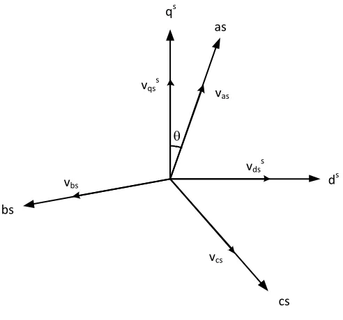
Consider a symmetrical three-phase induction machine stationary as-bs-cs axes at ⁄ angle apart, as shown in Figure 2-2. The goal is to transform the three-phase stationary reference frame variables into two-phase stationary reference frame variables (ds-qs) and then transform these to synchronously rotating reference frame (de-qe).
qs
ds as
bs
cs vas
vbs
vcs vqss
vdss
Figure 2-2 Axis transformation
[
] [ ( ) ( ) ( ) ( )
] [
] (2.2)
where is added as the zero sequence component, which may or may not be present.
If the angle is set to zero, the qs-axis aligns with the as-axis. Assuming the three phases are balanced and that the zero sequence component is not present, equation (2.2) (3.1) can be simplified as
√
√
√ ( )
(2.3)
Equation (2.3) can also be used to transform the stator currents from three-phase to corresponding equivalent two-phase quantities.
The synchronously rotating reference frame is at an angle with respect to the stationary reference frame. The transformation from the stationary reference frame to the synchronous reference frame is defined in equation.
[ ] [
] [
] (2.4)
2.3.2 DC motor analogy
In a dc machine, neglecting the armature reaction and the effect of field saturation, the torque developed by the motor can be defined in equation (2.5)(3.1).
(2.5)
current, the field flux ( ) is not affected and a fast torque response is possible. Similarly, changing the field current does not affect the armature flux ( ).
If the induction machine control is considered in a synchronously rotating reference frame, where the sinusoidal voltage and current variables appear as dc quantities in steady state, the dc motor analogy can be extended to the induction motor as well. The d-axis current is analogous to field
current and the q-axis current is analogous to the armature current of a dc motor.
Therefore, the torque can be expressed as
̅ (2.6)
or
(2.7)
This dc machine like behavior is possible only if is aligned in the direction of the flux and is
established perpendicular to it. Figure 2-3 shows a block diagram of a vector controlled induction motor drive. From the space vector diagram on the right of Figure 2-3, it can be seen that when
is controlled, it affects the q-axis current only, and does not affect the flux . Similarly, when
is controlled, it affects the flux only and does not affect the component of current. This vector or
field orientation of currents is essential under all operating conditions in a vector controlled drive.
IM
Inverter Vector
Control
*
e qs
i
* e ds
i
e qs
i
e ds
i
r
ˆFigure 2-3 Vector controlled induction motor
2.3.3 Principles of stator flux oriented vector control
then it is called direct vector control. The field angle can also be obtained using rotor position measurement and partial estimation with only machine parameters. This leads to a class of control schemes called indirect vector control.
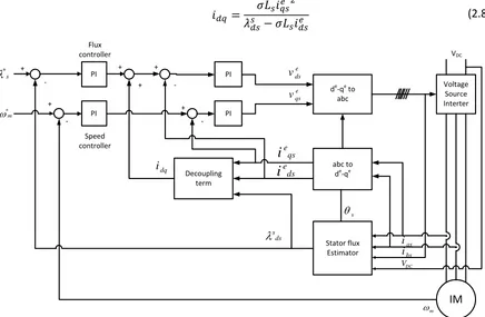
Figure 2-4 shows the block diagram of a stator flux oriented control method. Dependence on many machine parameters is greatly reduced when stator flux linkages are used and the electromagnetic torque is calculated using only stator flux linkages and the stator currents. Accurate estimation of stator flux is much easier than that of the rotor flux vector since only stator resistance is needed to calculate the value of the stator flux. However, in stator flux oriented control, the flux and torque producing currents are not naturally decoupled. The flux is a function of both and
currents. This means that if the torque is changed by , it will also change the flux. The coupling
effect needs to be dynamically eliminated by feed-forward control. Equation (2.8) defines the term to be added to the output of the flux controller to nullify the coupling effect. It can be seen that the decoupling term is a function of , and .
(2.8) IM Voltage Source Interter de-qe to
abc
Stator flux Estimator
Figure 2-4 shows a block diagram of a stator flux oriented control scheme. The flux and speed PI controllers produce the reference signals for the flux and the torque producing currents respectively in the synchronously rotating reference frame. Figure 2-4 shows the decoupling term is added to
the output of the stator flux controller to produce the reference current for the d-axis current
controller. The accuracy of the decoupling term can be affected by parameter variation.
However, since this term is in a feedback loop, this effect can be neglected [1]. The reference current signals are compared with the measured values of the d- and q-axis currents. Two PI regulators produce the required reference voltage signals that are fed in to the inverter.
2.4Direct Torque Control
Direct torque control (DTC) is an alternative approach to control of induction motors in high performance adjustable speed drives (ASDs). It makes use of specific properties of the induction motor for direct selection of consecutive states in the inverter. The selection of optimum inverter switching modes is made to restrict the torque and flux errors within respective torque and flux hysteresis bands, to obtain fast torque response, low inverter switching frequency and lower harmonic losses.
The electromagnetic torque in a symmetrical three-phase induction machine is proportional to the cross-vector product of the stator flux linkage and the stator current in the stationary reference frame [2]. Equation (3.1) shows the expression for electromagnetic torque.
( ̅ ̅ ) (2.9)
where ̅ is the stator flux linkage space vector and ̅ is the stator current space vector in the stationary reference frame. The term “P” is the number of pole pairs. From Figure 2-5, equation (3.9) can be rewritten as
| ̅ | | ̅ | ( ) | ̅ | | ̅ | (2.10)
ds qs
s
i
s
s
s
Figure 2-5 Stator flux-linkage and stator current space vectors
For a given rotor speed, if the modulus of the stator flux linkage is kept constant, and the angle is changed rapidly, then the electromagnetic torque can be quickly changed. If the actual developed electromagnetic torque is smaller than the reference value, the torque should be increased as fast as possible by using the fastest possible. However, when is equal to the reference, the rotation is stopped. If the stator flux-linkage vector is accelerated, positive torque is produced, and when it is decelerated, negative torque is produced.
To summarize, the electromagnetic torque can be quickly changed by controlling the stator flux-linkage space vector, which can be changed by using appropriate stator voltages. Thus, direct stator flux and torque control can be achieved. In contrast, in a vector controlled induction motor drive, the stator currents are used as control quantities.
ds
qs
) 100 (
1
v
) 110 (
2
v
) 010 (
3
v
) 011 (
4
v
) 001 (
5
v v6(101)
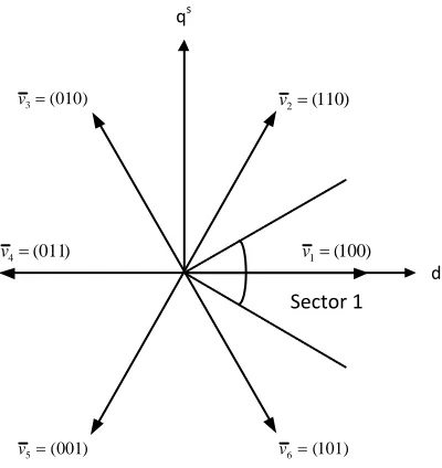
Figure 2-6 shows the six non-zero active voltage switching space vectors ( ̅ , ̅ , … ̅ ). These can be written as
̅ ̅ ( ( ) ) (2.11)
where is the dc-link voltage. The two zero space vectors ( ̅ , ̅ ) where the stator windings are
short circuited, ̅ . It follows from the definition of the switching vectors given above that since ̅ , ̅ is aligned with the real axis (ds – axis) of the stationary reference frame.
ds qs
Sector 1 Sector 2
Sector 3
Sector 4
Sector 5 Sector 6
s
2
sref
s
sref
1
P
0 P 2
P
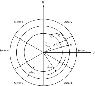
Figure 2-7 Control of Stator Flux
stator flux-linkage space vector is at the upper limit (| ̅ | ), it must be reduced. This can be
achieved by applying a suitable switching vector, which is the switching vector ̅ , as shown in Figure 2-7. Thus the stator flux-linkage space vector will move rapidly from point to , and it can be seen that point is in sector 2. It can be seen that at point the stator flux-linkage space vector is again at the upper limit. On the other hand, it should be noted that if the stator flux-linkage space vector moves in the clockwise direction from point , then the switching vector ̅ would have been selected, since this would ensure the required rotation and also the required flux decrease. Since at point , the stator flux-linkage space vector again reaches the upper limit, it has to be reduced when it is rotated in the anticlockwise direction. For this purpose, switching vector ̅ has to be selected, and then ̅ moves from point to as shown in Figure 2-7, which is also in sector 2. It should be noted that if, for example, at point a quick anticlockwise rotation is required, then it can be seen that the quickest rotation is achieved by applying the switching vector ̅ . On the other hand, if at point the rotation of the stator flux-linkage space vector has to be stopped, then a zero switching vector has to be applied, so either ̅ or ̅ can be applied.
Stopping the rotation of the stator flux-linkage space vector corresponds to the case when the electromagnetic torque does not need to be changed (reference value of electromagnetic torque is equal to its actual value). When the electromagnetic torque has to be changed (in the clockwise or anticlockwise direction), the stator flux-linkage space vector has to be rotated in the appropriate direction.
2.4.1 Control Strategy of DTC
The block diagram for direct torque control is shown in Figure 2-8. The speed control loop and the flux reference generator as a function of speed are shown in Figure 2-9. The speed controller utilizes a linear speed regulator producing the reference value . Linear speed regulators are typically of proportional-integral (PI) type. The flux reference is computed as a function of speed. Rated stator flux ( ) is demanded for speeds less than the rated speed ( ). At speeds higher than
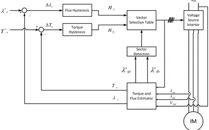
IM Voltage Source Interter Vector Selection Table Torque and Flux Estimator Sector Detection Torque Hysteresis Flux Hysteresis VDC + -+ e T s e T* s * e T s as i bs i DC V qs s
sds
H
e
T
H
Figure 2-8 Block diagram of a DTC controller
The command stator flux linkage ( ) and electromagnetic torque ( ) are compared to their respective estimated values, and the errors are processed through hysteresis-band controllers, as shown. The flux loop controller has two levels of digital output according to the following relations:
{ | ̅ | | ̅ | | |
| ̅ | | ̅ | | | (2.12)
m
w
mw
s *
eT
*Flux control scheme Speed control scheme
The torque loop has three levels of digital output, which have the following relations:
{
(2.13)
The feedback stator flux and electromagnetic torque are calculated from the machine terminal voltages and currents. The dc link voltage is measured and the machine terminal voltages are recreated from the switching pulses generated by the vector selector block. The sector number ( ) is calculated to identify the sector in which the stator flux linkage space vector lies. The voltage vector table block receives the input signals , and ( ) from the flux controller, the torque controller and the sector detector blocks respectively. Appropriate control voltage vector (switching states) for the inverter are computed by a look-up table as shown in Table 2-1.
Neglecting the effect of stator resistance of the machine, an incremental change in the stator flux linkage space vector can be written as:
̅ ̅ (2.14)
It can be seen that the stator flux linkage space vector will move fast if non-zero switching vectors are applied. For a zero switching vector, it will almost stop (it will move very slowly due to the small ohmic voltage drop). For a six-pulse VSI, the stator flux linkage moves along a hexagonal path with constant linear speed, due to the six switching vectors. In the DTC drive, switching vectors are selected on the basis of keeping the stator flux linking errors within the required tolerance band, and keeping the torque error in the hysteresis band. It is assumed that the widths of the two hysteresis bands are and respectively. If the flux vector lies in the sector, then its magnitude can be increased by using the space vectors ̅ , ̅ , and ̅ . The magnitude of the
stator flux linkage can be decreased by selecting ̅ , ̅ , and ̅ . The selected voltage vectors
between the zero and non-zero vectors. It is important to note that the duration of the zero states has a direct impact on the electromagnetic torque oscillations [2].
Table 2-1 Optimum voltage switching vector look-up table
( ) ( ) ( ) ( ) ( ) ( )
1
1 ̅ ̅ ̅ ̅ ̅ ̅
0 ̅ ̅ ̅ ̅ ̅ ̅
-1 ̅ ̅ ̅ ̅ ̅ ̅
0
1 ̅ ̅ ̅ ̅ ̅ ̅
0 ̅ ̅ ̅ ̅ ̅ ̅
-1 ̅ ̅ ̅ ̅ ̅ ̅
In a DTC induction motor drive, the stator flux linkage components need to be estimated due to two reasons. First, these components are required in the optimum switching vector selection table described in this section. Secondly, they are also required for the estimation of electromagnetic torque. Stator flux estimation is discussed in more detail in Chapter 3.
2.4.2 Simulation of DTC Controller
A direct torque control algorithm was implemented in simulation based on the ideas discussed above. The software package Matlab/ Simulink® was used to implement the proposed algorithm for a 3-phase induction motor model. The “SimPowerSystems” toolbox available in Simulink was used to model the power electronics components.
Figure 2-10 Simulink block diagram of DTC algorithm
Figure 2-11 Rotor speed in rpm and electromagnetic torque in Nm
The speed reference is compared with the speed feedback signal to produce a speed error. This quantity is processed through a PI regulator to produce the reference signal for the electromagnetic torque. This reference signal is compared with the estimated torque and processed though a torque
Flux reference speed Psi_qs Psi_ds m sector determinator Continuous powergui psisn sector K dTe dpsi new vector Vector selector Torque error - sign Speed ref
Sign=1 -> 1 Sign=1 -> 0
Sign=1 -> 1 Sign=1 -> 0
sel. vect ua ub uc SVPWM Inverter a b c psi_qs psi_ds speed Torque psi Is_a Induction Motor 60 -K-Flux error - sign PI Discrete PI Controller Flux error Torque error Torque error
0 0.5 1 1.5 2 2.5 3 3.5 4 4.5 5
0 50 100 150 200 time (s) wm ( rp m )
0 0.5 1 1.5 2 2.5 3 3.5 4 4.5 5
estimated value of the stator flux. This error signal is processed by the flux hysteresis controller. The outputs of the two hysteresis controllers along with the sector information are fed in to the “vector selector” block. This block has the look-up table described in Table 2-1. The output of the “vector selector” block is synthesized by the SVPWM inverter block to produce the voltage signals to be fed in to the motor.
Figure 2-12 Stator flux linkage vector. 1) q-axis component of stator flux. 2) d-axis component of stator flux. 3) magnitude of stator flux linkage vector.
Figure 2-11 shows a plot of the rotor speed and the developed electromagnetic torque. Figure 2-12 shows the plot of the stator flux linkage vector as a function of time. The first sub-plot shows the q-axis component of the stator flux in the stationary reference frame. The second sub-plot shows the d-axis component of the stator flux. The magnitude of the stator flux is plotted in the third sub-plot. It can be seen that the magnitude of the stator flux remains constant
0 0.5 1 1.5 2 2.5 3 3.5 4 4.5 5
-1 -0.5 0 0.5 1
time (s)
s qs
(
W
b
)
0 0.5 1 1.5 2 2.5 3 3.5 4 4.5 5
-1 -0.5 0 0.5 1
time (s)
s ds
(
W
b
)
0 0.5 1 1.5 2 2.5 3 3.5 4 4.5 5
0 0.2 0.4 0.6 0.8
time (s)
s
(
W
b
Figure 2-13 Stator current at
Figure 2-14 Trajectory of stator flux
Figure 2-13 shows a plot of the stator current and Figure 2-14 shows the trajectory of the stator flux in the stationary reference frame. The d-axis component of the stator flux in the stationary reference frame is plotted on the x-axis, and the q-axis component is plotted on the y-axis.
0 0.5 1 1.5 2 2.5 3 3.5 4 4.5 5
-80 -60 -40 -20 0 20 40 60 80 time (s) Is ( A )
-1 -0.8 -0.6 -0.4 -0.2 0 0.2 0.4 0.6 0.8 1 -1 -0.8 -0.6 -0.4 -0.2 0 0.2 0.4 0.6 0.8 1
d-axis component of stator flux
Chapter 3
Flux and Torque Estimation
3.1 Introduction
In this chapter, the stator flux and torque equations will be derived and formulated in the reference frame fixed to the stator-flux linkage space vector. The open loop flux estimator is explained in section 3.2. Problems associated with using the open loop estimator are discussed in section 3.3. Each of the issues causing errors in flux estimation has been explained in detail.
3.2 Open loop flux estimators
The stator flux space vector is obtained by the integration of the difference of the terminal voltage and the stator ohmic voltage drop.
̅ ̅ ̅ ̅ ( ̅ ̅ )
(3.1)
Here, ̅ denotes the stator-flux space vector and is the stator resistance. Figure 3-1 shows a block diagram description of the flux estimator. The flux error is calculated from the difference of the reference value of the stator-flux and the estimated value. The flux error acts as the input to the hysteresis controller.
X
Rs
Flux Estimator
ʃ
λsλ* s
Δ λs
λ* s vs
(vs – is Rs)
is
Figure 3-1 Flux Estimator block
( )
( )
(3.2)
where ̅ , ̅ and ̅ .
The values of the direct- and quadrature axis of the stator voltages and currents in (3.2) can be obtained from the corresponding 3-phase quantities as follows:
√ ( ) √ ( )
(3.3)
√ ( ) √ ( )
(3.4)
The voltage and the currents are assumed to be balanced. Hence the zero sequence components do not exist. The angle of the stator flux-linkage vector can be obtained from the dq- axis as follows
(
). (3.5)
The electromagnetic torque is given by,
( ) (3.6)
where P is the number of poles.
3.3 Flux estimation problems
It should be noted that the accuracy of the estimated flux vector depends on the accuracy of the measured voltages and currents. The most important reasons that can cause incorrect flux estimation can be enumerated as follows:
1. Time delay (dead-time) between switching OFF of one device and switching ON of the other device on the same inverter leg.
2. Nonlinear characteristics of the PWM inverter which cause differences between the reference voltage and the output of the inverter.
Figure 3-2 Ideal flux and torque estimation. Open loop V/f control, stator frequency - 5Hz
Figure 3-2 shows a plot of the estimated stator flux and electromagnetic torque at no load. The effect of each of these issues mentioned above has been discussed in detail in this section.
3.3.1 Dead time
Due to definite turn-off and turn-on times of the switching devices in PWM inverters, it is necessary to insert a time delay between the switching OFF of a device and the switching ON of the other device on the same inverter leg. Figure 3-3 shows one phase of a PWM inverter
PWM
Generator
i
a VDC gate gate D1 T1 D2 T2Figure 3-3 Single phase configuration of PWM inverter -2 -1.5 -1 -0.5 0 0.5 1 1.5 2
-2 -1.5 -1 -0.5 0 0.5 1 1.5 2
d-axis component of stator flux (Wb)
q -a x is c o m p o n e n t o f st a to r fl u x ( W b )
4 4.2 4.4 4.6 4.8
Figure 3-4 shows the time delay (tdead) between the switches T1 and T2. . TON is the time for which
the switch T1 is ON. TSW is the switching period. At time t1, T2 transitions from ON to OFF. The
turning ON of T1 is delayed by time tdead. This prevents the short circuit across both the switches of
the inverter leg and the input dc voltage source. The introduction of the time delay between switching leads to reduced and distorted voltage at the output of the inverter.
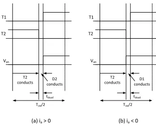
To examine the effect of dead-time on the output voltage, switching waveforms on one leg of the inverter are examined. The current is positive in the direction of the load. The IGBTs T1 and T2 conduct when they are ON. During the dead-time period, when both T1 and T2 are OFF, either the reverse recovery diode D1 or D2 will conduct depending on the direction of .
T1 T2 T1 T2
tdead
Ideal switching
Switching with dead-time
TON
Tsw
t1 t2
Figure 3-4 Time delay between turn OFF and turn ON of two switches on the same inverter leg
Depending on the direction of the switching transition and the sign of the current , four conditions are possible. Each of the possibilities is discussed below.
condition results in the correct voltage being applied to the motor terminals. Figure 3-5(a) shows the output voltage waveform during the transition.
The current is negative, T1 transitions from ON to OFF, T2 transitions from OFF to ON:
During the dead-time period, D1 continues to conduct and D2 blocks the flow of current. Thus, this condition results in a gain in the voltage being applied to the motor terminals. Figure 3-5(b) shows the output voltage waveform during the transition.
The current is positive, T1 transitions from OFF to ON, T2 transitions from ON to OFF: During the dead-time period, D2 continues to conduct and D1 blocks the flow of current. Thus, this condition results in a loss of voltage being applied to the motor terminals. Figure 3-6(a) shows the output voltage waveform during the transition.
The current is negative, T1 transitions from OFF to ON, T2 transitions from ON to OFF: During the dead-time period, D1 continues to conduct and D2 blocks the flow of current. Thus, this condition results in the correct voltage being applied to the motor terminals. Figure 3-6(b) shows the output voltage waveform during the transition.
Van
T1
T2
tdead
Tsw/2
T1
conducts conductsD2
(a) i
a> 0
Van
T1
T2
tdead
Tsw/2
T1
conducts conductsD1
(b) i
a< 0
In each switching cycle, T1 transitions from OFF to ON (T2 from ON to OFF) once and from ON to OFF (T2 from OFF to ON) once. Due to the distortions discussed above, the output voltage of the inverter is not equal to the desired reference voltage. In order to overcome the effect of dead-time, various approaches have been suggested. The compensation techniques can be broadly classified into two categories. In the first category, the voltage error is averaged over an entire cycle and in the second category, the voltage error is evaluated within the PWM pattern. The methods based on averaging theory look to modify the reference voltage by adding the average value of the voltage lost/gained due to the dead-time effect [3-5].
Van
T1
T2
tdead
Tsw/2
T2
conducts conductsD2
(a) i
a> 0
Van
T1
T2
tdead
Tsw/2
T2
conducts conductsD1
(b) i
a< 0
Figure 3-6 T1 transition from OFF to ON, (a) ia is positive. (b) ia is negative
distortion at the zero crossing regions. This solution, however, requires accurate detection of current. In [8], the analysis of the zero current clamping phenomena is discussed and the compensation method to eliminate zero current clamping is proposed. The PWM strategy in [9] presents a solution to the zero current clamping problems, but it requires extra hardware and a special PWM pattern in the neighborhood of zero crossing current. This PWM strategy restricts the number of switchings in the phase switches which convey the quasi-zero current to a small value. This increases the current ripple when the current is nearly zero.
The compensation technique presented in [6] was implemented both in simulation and in hardware. Experimental results will be discussed in section 6.1. The simulation results of the implementation are presented here. Figure 3-7 shows the Simulink model of the implemented algorithm on an open-loop Volts-Hertz controlled induction motor drive. A fixed step size of 100 s was used for simulation. The parameters for the induction motor used are the same as the actual motor on which hardware implementation is done. The motor was excited by a voltage with a stator frequency of 5Hz and amplitude corresponding to the rated V/f ratio. The amplitude of the input voltage was compensated for the drop in voltage due to the stator resistance. This effect is more prominent at low speeds when the magnitudes of the two voltages are comparable. The machine is operated at no-load conditions. The effects of the nonlinear behavior of the inverter have not been considered.
Figure 3-7 Simulation - Simulink model of dead-time compensation implementation rpm
-K-rad/s to rpm
Continuous powergui is_a 5 fs 100 Vdc1 Vdc+ Vdc-Vdc Vm f Vdc Iabc Vabc duty_a_b_c
V/f to duty
Figure 3-8 shows the “V/f to duty” block from Figure 3-7. The reference value is normalized by the dc link voltage and three sinusoidal signals phase shifted by 120o at the stator frequency is
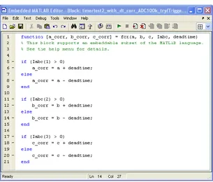
generated. These act as duty ratios for the gate signals of the PWM inverter. The maximum and minimum values of the three duty signals (a, b and c) are limited to 95% and 5%. These signals are fed to the dead-time compensator block, shown in Figure 3-9, along with the measured stator currents and the value of the dead-time introduced in the input to the PWM inverter.
Figure 3-8 Simulation - block diagram of "V/f to duty" block
1 duty_a_b_c a
b
c
Iabc
deadtime
a_corr
b_corr
c_corr
deadtime compensator 0.01
deadtime c limit u(1)*cos(u(2)+2*pi/3)+0.5
c
b limit u(1)*cos(u(2)-2*pi/3)+0.5
b
a limit u(1)*cos(u(2))+0.5
a
f wt
Subsystem Divide
4 Iabc 3
Vdc
The ideal pulse ON-time is modified based on the sign of the current though that phase. If the phase current , then the compensation algorithm adds the dead-time to the ideal ON-time. The corrected pulse is processed through the dead time generator. The resulting pulse position not symmetric and is shifted by one-half the dead-time. If the phase current , then the compensation algorithm subtracts the dead-time to the ideal ON-time.
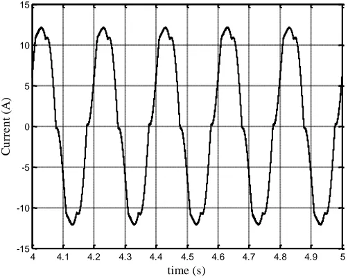
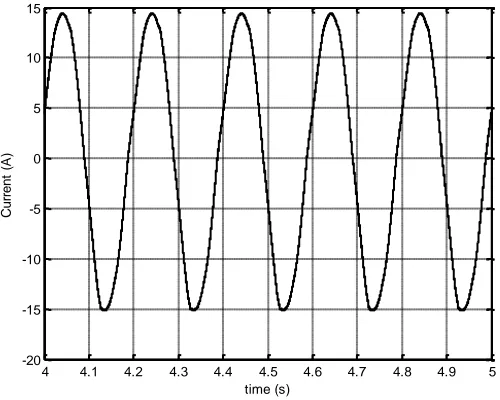
Figure 3-10 Stator current with 1 s dead-time; without dead-time compensation
Figure 3-11 Estimated stator flux and electromagnetic torque with 1 μs dead-time; without dead-time compensation
Figure 3-10 shows the effect of dead-time on the stator current. The stator current waveform is distorted. Figure 3-11 shows a plot of the estimated stator flux and electromagnetic torque with an
4 4.1 4.2 4.3 4.4 4.5 4.6 4.7 4.8 4.9 5 -15 -10 -5 0 5 10 15 time (s) C u rr e n t (A )
-1 -0.5 0 0.5 1
-1 -0.8 -0.6 -0.4 -0.2 0 0.2 0.4 0.6 0.8 1
d-axis component of stator flux (Wb)
q -a x is c o m p o n e n t o f st a to r fl u x ( W b )
4 4.2 4.4 4.6 4.8 5
uncompensated dead-time of 1 . In the estimated stator flux trajectory plot, the dotted circle represents the estimated trajectory of the flux under ideal conditions. The solid circle represents the estimated flux trajectory when a time delay between switching is present, and has not been compensated for.
Figure 3-12 Stator current with 1 s dead-time; with dead-time compensation
Figure 3-13 Estimated stator flux and electromagnetic torque with 1 μs dead-time; with dead-time compensation
Figure 3-12 shows the waveform of the stator current with the dead-time compensation algorithm 4 4.1 4.2 4.3 4.4 4.5 4.6 4.7 4.8 4.9 5
-20 -15 -10 -5 0 5 10 15 time (s) C u rr e n t (A )
-1 -0.5 0 0.5 1
-1 -0.8 -0.6 -0.4 -0.2 0 0.2 0.4 0.6 0.8 1
d-axis component of stator flux (Wb)
q -a x is c o m p o n e n t o f st a to r fl u x ( W b )
4 4.2 4.4 4.6 4.8 5
the motor. Thus, the magnitude of the stator current is higher when correct gate signals are applied. Figure 3-13 shows the plot of the estimated stator flux trajectory and the estimated electromagnetic torque when the dead-time compensation algorithm is operational. It can be seen that the estimated flux trajectory and the ideal estimated flux trajectory are very close to each other. Also, the pulsation in the estimated electromagnetic torque is substantially lower.
3.3.2 Stator resistance variation
The primary reason for the misalignment of the estimated stator resistance with its real value is thermal drift of motor parameters. Load dependent variations of the winding temperature may result in the stator resistance changing from 0.5 to 1.5 times the modeled value. The effect of using an incorrect value of stator resistance for flux estimation has been discussed by several scholars [10]. This effect is more prominent at low speeds [11, 12]. Several methods to estimate the variation in stator resistance with temperature have been presented based on state observers, PI and fuzzy controllers [13, 14]. For accurate flux estimation, the estimated value of stator resistance should be continuously adapted for temperature changes.
A decrease in the stator resistance of the motor leads to larger currents in the stator windings for the same input voltages. This results in increased flux and electromagnetic torque generation in the motor. Let the value of the stator resistance decrease by to ( ). If the flux and electromagnetic torque references do not change, this will result in an increase in the stator current by . Thus (3.1) can now be re-written as
̅ ( ̅ ( )( ̅ ̅ )
(( ̅ ̅ ) ( ̅ ̅ ̅ ))
((( ̅ ̅ ) ( ̅ )) ( ̅ ̅ ))
(3.7)
If the flux estimator uses the constant value of the stator resistance, the equation for estimated flux can be written as
̂̅ ( ̅ ( ̅ ̅ ))
(( ̅ ̅ ) ( ̅ )) (3.8)
̅ ̅ ̂̅
( ̅ ̅ ) (3.9)
The estimated value of the flux is smaller than the actual value by ̅ . A decrease in the stator resistance results in a positive stator flux error. Since the electromagnetic torque is calculated using (3.6), the estimated value of the electromagnetic torque will also be lower than the actual value.
Open loop flux Volts-Hertz control algorithm was implemented and stator flux and torque were estimated. Six different values of stator resistance were used - , , , and . The value of the stator resistance used for estimating the stator flux and the electromagnetic torque was for all the cases. Figure 3-14 shows a plot of estimated stator flux and electromagnetic torque for each case. It can be seen that there is offset in the estimated stator flux, and there is significant oscillations in the estimated torque. The oscillations are higher when the value of decreases from its nominal value.
Figure 3-14 Estimated stator flux and electromagnetic torque; stator resistance variation from 50% to 150% of original value
When a closed loop flux controller is used, in a vector control or direct torque control (DTC) algorithm, the offset in stator flux estimation will produce an error signal even when the real value of the stator flux is equal to the reference value. This error signal will cause the controller to increase (or decrease) the input voltage to the motor to minimize the error. This would lead to an
-2 -1 0 1 2
-2 -1.5 -1 -0.5 0 0.5 1 1.5 2
d-axis component of stator flux (Wb)
q -a x is c o m p o n e n t o f st a to r fl u x ( W b )
5 5.2 5.4 5.6 5.8 6
-30 -20 -10 0 10 20 30 time (s) E st im a te d E le c tr o m a g n e ti c T o rq u e ( N m
) 0.50 Rs
0.75 Rs
1.00 Rs
1.25 Rs
of the flux and the electromagnetic torque. This positive feedback can lead to an unstable system leading to a runoff condition.
3.3.3 Voltage drop in power electronic devices
At low speeds, the voltage distortions caused by the nonlinear behavior of the PWM inverter become significant [15]. This is due to the forward voltage drop of the power devices when they conduct. This can be modeled by an average threshold voltage and an average differential
resistance as marked by the dotted line in Figure 3-15.
0 1 2 3 4 5
10 20 30 40 50 60 70 80 90 100
vth
VCE [V]
IC
[
A
]
25oC
125oC
rd
Figure 3-15 Inverter output characteristics. Dotted line: modeled approximation. (Reproduced from Product datasheet - BSM50GP120, Infineon)
The differential resistance can be viewed as a series quantity that adds to the stator resistance. The effect of uncompensated differential resistance on the estimated flux and electromagnetic torque is the same as that when an increase in the stator resistance is not compensated.
The effect of the threshold voltage, however, is nonlinear and requires a study of the inverter model. Depending on the switching state of the inverter, the stator phase currents will flow through an active device or through a reverse recovery diode. The direction of the phase currents does not change in a larger interval of one-sixth of a fundamental cycle. The effect of the threshold voltages does not change as the switching states change. The inverter always introduces a voltage component of identical magnitude ( ) to all the three phases. The sign of the voltage component
is determined by the direction of the phase currents. The voltage threshold vector can be defined as
where ( ). Equation (3.10) can be re-written as
̅ ( ̅ ) (3.11)
where
( ̅ ) ( ( ) ( ) ( )) (3.12)
is the sector indicator. The sector indicator defines the 60o sector where ̅ is located.
The value of the stator voltage estimated from the dc bus voltage and the PWM switching signals can now be modified as
̂̅ ̂̅ ( ̅ ̅ ) (3.13)
The term ̂̅ represents the actual voltage at the terminals of the motor.
Figure 3-16 shows a plot of the estimated stator flux trajectory and the estimated electromagnetic torque when inverter nonlinearities are present. It can be seen that the estimated flux trajectory is lower than the ideal trajectory. Figure 3-17 shows the stator current when inverter nonlinearities are present and have not been compensated. Compensation of inverter nonlinearity based on the description above is discussed in section 6.1.
Figure 3-16 Estimated stator flux and electromagnetic torque when inverter nonlinearities are present
-1 -0.5 0 0.5 1
-1 -0.8 -0.6 -0.4 -0.2 0 0.2 0.4 0.6 0.8 1
d-axis component of stator flux (Wb)
q -a x is c o m p o n e n t o f st a to r fl u x ( W b )
4 4.2 4.4 4.6 4.8 5
Figure 3-17 Stator current when inverter nonlinearities are present
3.3.4 Measurement errors in sensors
Switching frequencies of PWM inverters today are much greater than the electric time constant of the motor. Thus, it is possible to measure the dc link voltage and reconstruct the phase voltages from the voltage reference signal available inside the digital controller. This voids the need to measure each of the phase voltages separately. The result of measuring the dc link voltage instead of the phase voltages means that the nonlinear behavior of the inverter has to be modeled and accounted for. This effect is more prominent at low speeds, where the inverter output voltage is low.
The following problems can be associated with measurement of the stator currents and voltages:
1. Uncompensated measuring offset 2. Unequal sensor gains
3. Quantization noise introduced by non-ideal A/D converter
4. High frequency harmonics in the measured signal – these are the consequence of discrete inverter output voltage
5. Phase lagging introduced by measuring low pass filter
4 4.1 4.2 4.3 4.4 4.5 4.6 4.7 4.8 4.9 5 -20
-15 -10 -5 0 5 10 15 20
time (s)
c
u
rr
e
n
t
(A
The first two points predominantly describe the sensor characteristics in an electric drive control structure [16]. Various solutions have been suggested in literature to eliminate this influence. The most common approaches include feed-forward offset correction and calibration [2]. The sensors are calibrated every time the drive is started. For this purpose, during the calibration stage (prior to starting up the drive), average offset values of voltages and currents can be obtained by taking hundreds of readings. During normal operation of the drive, these average values are then subtracted from the measured values. However, sensor or ambient warm-up during drive operation causes a thermal drift in sensor output, which causes sensor output values to be slightly different from the values stored in memory during the calibration stage.
Use of a low pass filter application with adaptive time constant is suggested instead of an ideal integrator for stator flux estimation [17]. Using this approach, the authors were able to achieve 30 second long torque control for 0.005 p.u. relative stator frequency. Shin et al. in [18] propose using a programmable low pass filter with phase compensation. The phase compensation angle is adjusted to give right angle between the estimated stator flux and the electromotive forces. Bose and Patel in [19] suggest the replacement of the integrator with a software programmable cascade of low pass filters. They reported two problems – increased computational requirements and low frequency instability (below 0.5 Hz).
In [20], Hu and Wu present three algorithms for flux estimation in high performance drives. The idea is based on adaptively introducing correction signals. The differences between algorithms are the methods used to calculate the correction signals. In the first algorithm, a modified integrator with a saturable feedback is used. This requires additional processing of the estimator output. The second algorithm computes the correction signal in the synchronously rotating reference frame. In the third method, the correction signal is applied with the intention to correct the angle between the estimated flux and the stator electromotive forces to 90o for appropriately estimated stator flux vector.
decreases. Multi-motor speed regulation in 1:100 speed range with an accuracy in speed regulation better than 0.1% have been reported.
A comprehensive method directed towards solving the problems of flux estimation considering all the main sources of error – the effect of offset error, scaling error, parameter mismatch and inverter non-linearity is discussed in [22] and [23]. The offset compensation term is calculated by measuring the flux trajectory dislocation from the origin during the period of stator flux signal. The switches are modeled and the output voltage loss due to the conducting switches is compensated. Real-time identification of stator resistance is employed and error due to dead-time is compensated. As a consequence, an ideal integrator could be used for flux estimation leading to a significantly wider regulation bandwidth. Drive operation at 0.0003 p.u. relative stator frequency, drive starting after a long standstill period, and speed reverse operation have been reported.
In [24], the impact of current measurement error is analyzed on the characteristics of current regulated indirect vector controlled drive. Oscillation in motor torque caused due to offset and scaling error is discussed and feed forward compensation method based on spectral analysis of measured speed is suggested. The explained method is able to reduce the amplitude of the first and second harmonic speed oscillations to approximately one-third of the uncompensated value.
Chapter 4
Proposed Algorithm for Sensor Offset
Identification and Correction
4.1 Introduction
In this chapter, a new flux and torque estimation algorithm is presented. In section 4.2, the influence of voltage and current sensor dc offset on stator flux and electromagnetic torque estimation is explained. In section 4.2, an algorithm intended for high precision flux and torque estimation in drives where the current and/or voltage sensors have unknown offset error is introduced. The main characteristic of this algorithm is its ability to recognize the sensor(s) that introduces the error and to estimate the error. The algorithm is able to compensate the offset error at its source. Thus, all estimation/compensation blocks which need the stator currents and voltages as inputs will have access to error-free quantities.
4.2 Influence of voltage and current sensor dc offset on flux and torque
estimation
Equations (3.1) and (3.2) can be used to estimate the value of stator flux as follows:
̂̅ ̂̅ ( ̂ ̂ ) (4.1)
̂ ̂ ( ̂ ̂ )
̂ ̂ ( ̂ ̂ )
(4.2)
The terms ̂̅ , ̂ and ̂ denote the estimated values of the stator flux. The “^” sign above the
and the terms are used to denote measured values of voltages and currents. Further, ̂ and ̂
represent the estimated value of the stator flux vector before time t=0, when the estimation started.
applications. However, implementation of an integrator for motor flux estimation is quite complicated. A pure integrator will accumulate dc drift and has initial value problems. Any discrepancy between model parameter Rs and the motor stator resistance directly influences the
value of the estimated flux. The lower limit of the basic open-loop flux estimation is reached when the stator frequency is around 3-5Hz.
When currents and/or voltages sensors introduce offsets ( , , , ), the relation between
the measured quantities ( ̂ , ̂ , ̂ , ̂ ) and the real (actual) measured quantities ( , , , )
can be described as:
̂ ̂ ̂ ( ̂ ̂ ) ( )
}
̂ ̂
√ ( )
(4.3)
̂ ̂ ̂ ( ̂ ̂ ) ( )
}
̂ ̂
√ ( )
(4.4)
Since the three phases of the input voltage and current are assumed to be symmetric, the “c” component of the phase current is not measured. It is calculated from the “a” and “b” phase currents. If the “a” and “b” phase sensors have measurement offsets, then the offset in the third phase is a linear combination of the first two phases, as is shown in (4.3). It should be noted that the effect of measuring voltage offset ( ) on estimated flux is the same as the following offset
in measured current:
* + (4.5)
Equations (4.1) and (4.2) show that the cumulative effect of the integration process results in deterioration of the estimated trajectory of stator flux even for very small value of measuring offset. The deterioration can be identified when the center of the estimated flux vector starts to deviate from the origin. If an appropriate self-commissioning procedure is applied, the main cause of measurement offset is thermal drift in sensor electronic components. The thermal drift time constant is much larger than the electric time constant of the induction motor. Thus, the offset in current measurement can be treated as a constant vector which translates the circular trajectory of estimated flux away from the origin. The shape of the final flux trajectory is the combined effect of accumulated offset and a limiter which is a standard part of the flux estimator. Figure 4-1 presents the effect that current offset has on estimated trajectory of stator flux. The saturation effect protects the trajectory of estimated flux from drifting further away from the origin.
Figure 4-1 Estimated stator flux when non-zero sensor dc offset is present
Assuming that the bandwidth of the current loop is wide enough, the current error at the input to the current regulator can be expected to be zero.
̂ ̂
̂ ̂ (4.6)
This means that the result of the current measurements will exactly follow the reference values.
-2 -1 0 1 2
-2.5 -2 -1.5 -1 -0.5 0 0.5 1 1.5 2 2.5
component of stator flux (Wb)
c o m p o n e n t o f st a to r fl u x ( Wb )
d-axis component of stator flux (Wb)
windings will be different than the commanded values. The terms and in (4.7) denote the
current measurement offset transformed into the synchronously rotating rotor flux oriented reference frame.
(4.7)
From (4.8), a conclusion can be drawn that in steady state a constant dc current sensor offset produces sinusoidal d and q components with a stator frequency, .
√ √ (
√
)
√ √ ( √
)
(4.8)
The amplitude is directly proportional to the length of current offset vector and the phase is shifted from the phase of the rotor flux by the current offset error phase angle.
Electromagnetic torque ( ) can be estimated in the rotor flux oriented reference frame using (4.9), where P is the number of pole pairs, is the magnetization inductance, is the rotor inductance and is the rotor flux entirely positioned along the d-axis ( ).
(4.9)
Equation (4.10) describes the relation between the d-axis stator current and the rotor flux. A periodic variation in will cause a corresponding variation in . The rate of these variations is described by the rotor time constant . If the stator frequency is typically above 5Hz, the rotor flux can be safely assumed to be “inert” towards variations in , and to be approximately equal to the reference value .
(4.10)