Modelling and Finite Element Analysis of
Double Wishbone Suspension
Amol Patil , Varsha Patil,
Prashant Uhle
P.G. Student, Dept. of Mechanical Engineering, S S B T S College of Engineering, Ja lgaon, Maharastra, India
P.G. Student, Dept. of Mechanical Engineering, J N E C College of Eng ineering , Aurangabad, Maharastra, India
Assist. Professor, Dept. of Mechanica l of Eng ineering, SSBTS Co llege of Engineering Ja lgaon Maharastra, India
Abstrac t: Automobile systems today is going through major changes and as concert to comfort the suspension system
and its working is very impo rtant. The study of suspension system and dynamic analysis are discussed in this paper.
The links of the suspension are assumed to be fle xible and the elastic stiffness, mass, and geometric stiffness matrices
are obtained by using Finite Ele ment Method .In order to e xpress the linear equation of mot ion, suspension link forces
required for the geometric stiffness matrices are assumed as constant. Also, the oscillations of the suspension links are neglected since the base displacement is chosen in sma ll a mp litude. The FEA done by divid ing the lo wer and the upper
arms into two e le ments . Double wishbone suspension of a quarter cars is modelled assuming the suspension links to be
rig id.
Keywor ds— double wishbone suspension system, Modelling, Dyna mic analysis, Finite Ele ment Method.
I.INTRODUCTION
Now a day’s nearly all types of passenger cars and light trucks use independent front suspensions, because of the better
resistance to vibrations. One of the commonly used independent front suspension system is referred as double
wishbone suspension. The quarter car with the double wishbone suspension system is modelled for two different
approaches to the suspension links as rigid and fle xib le. The refore, the dynamic analyses of these models are investigated by the finite e le ment method. This paper deals with the analytical method and the finite ele ment method. The ele ment stiffness, the mass and the geometric matrices are e xp lained for the plane fra me e le ment respectively. Modelling of double wishbone suspension is presented in two models. Vibrat ions of the double wishbone suspension system, natural frequencies and response to base excitat ion are studied.
In Fin ite Ele ment Method, a comple x region defin ing a continuum is discredited into simp le geometric shapes called fin ite e le ments. The materia l properties and the governing re lationships are considered over these elements and expressed in terms of unknown values at the nodes. An assembly process, duly considering the loading and constraints, results in a set of equations. Solution of these equations gives us approximate behaviour of the continuum use of the analytical method and finite ele ment method for the dynamic analysis of double wishbone suspension system is described. Mass, stiffness and geometric stiffness matrices are derived. The plane fra me e le ment is selected to model the double wishbone suspension me mbers.
II.CHARACTERIS TIC MATRICES OF THE PLANE FRAME ELEMENT
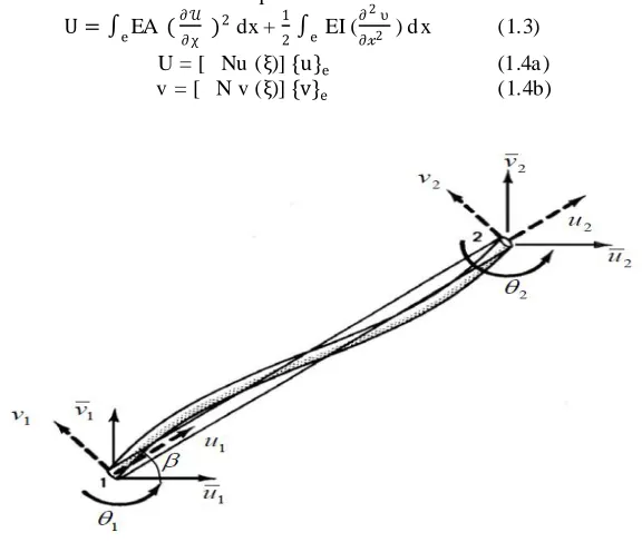
A planar (2-D) fra me e le ment is subjected to both axia l and bending deformations. Therefore , the plane fra me e le ment
has three degrees of freedom per node together with loca l d isplacements (u 1, v1 and θ1) and g lobal d isplace ments (ū 1,
v1 and θ1) as shown in Figure 1.1. The nodal d isplacement vector is given by
{q}= {u1 v1 θ1 u2 v2 θ2} T (1.1)
The ele ment stiffness matrix for a 2-D fra me e le ment can be constructed by superimposing both axia l and bending stiffness. The element kinetic and strain energy functions for plane fra me ele ment are given in terms of local coordinates, as follows; given in terms of loca l coordinates as follows;
T = 1
2 ∫e ρ A (u
-2
+ ν- 2) d x (1.2)
Where the over dot shows the differentiation with respect to time.
U = ∫eEA ( ∂ 𝒰
∂ χ )
2 dx + 1
2∫e EI (
∂2 υ
∂𝓍2 ) d x (1.3)
U = [ Nu (ξ)] {u}e (1.4a )
v = [ N v (ξ)] {v}e (1.4b)
Figure 1.1. Plane frame element (Source: Belegundu and Chandrupatla 1997)
III.ELAS TIC STIFFNESS MATRIXES
Substituting the displacement functions given in Equation (1.3) into strain energy e xpression given in Equation ( 1.4) gives,
T=
12
{
ū
}
e T[m]
e
{
ū
}
e (1.5)(1.6)
[k]
e =𝐸𝐼𝑧
2𝑎2
Where,
l
e= 2a and
𝑟
𝑧2= 𝐼
𝑧/ A [ 10]
IV.GEOMETRIC STIFFNESS MATRIX
The geometric strain energy in the ele ment is
𝑈
𝑔=
∫
𝑃 2 𝐿𝑂
(
𝜕𝑣
𝜕𝑥
)
2
dx =
12
{𝑞}
𝑇
[𝑠]
𝑒
{q} (1.7)
The geometric stiffness matrix [s] for a p lane fra me is developed from the Equation (1.7)
(𝑎 𝑟 )2 2 0 0 −(𝑎 𝑟 )2 2 0 0
0 3 3a 0 -3 3a
0 3a 4𝑎2 0 -3a 2𝑎2
0 0 (𝑎 𝑟 )2 2 0 0
0 -3 -3a 0 3 -3a
(1.8)
[s]e =
𝑃 60𝑎
Where,
l
e = 2a and P is the a xial force [4 ]V.MASS MATRIXES
Substituting the displacement functions given in Equation (1.4) into the kinetic energy e xpression given in Equation (1.2) gives
T=
12
{
ū
}
e T[m]
e
{
ū
}
e( 1.9)
Where[m]
e=
ρAa105 (1.10)
In which
l
e = 2a, ρ is the mass per unit volume, and A is the cross -sectional area of each ele ment [10 ]VI.STIFFNESS OF THE SPRING
In finite e le ment model, stiffness of helical-shaped springs used in suspension system may be e xp ressed in matrix notation considering the plane fra me e le ment displace ment vector as follows;
[𝑘𝑠] = k (1.11)
Where k is the stiffness coefficient of the spring by the equation;
𝑘 =
𝐺𝑠𝑑464𝑛𝑅𝑠3
(1.12) Where,
The stiffness is a function of the shear modulus (Gs), the dia meter of the turns of coils (Rs), the dia meter of the coils (d), and the number of the coils (n) [14]
VII.COORDINATE TRANS FORMATIONS
If a fra me me mber is inclined in g lobal coordinate system as shown in Figure 3.1, the e le ment stiffness, mass and geometric stiffness matrices require the p lanar t ransformat ion. Figure 3.1 shows the nodal freedo ms in local and global systems. The relation between the local and global displace ments is
0 0 0 0 0 0
0 36 6a 0 -36 6a
0 6a 16𝑎2 0 -6a −4𝑎2
0 0 0 0 0 0
0 -36 -36 0 36 -6a
0 6a 6a 0 -6a 16𝑎2
70s 0 0 35 0 0
0 78 22a 0 27 -13a
0 22a 8𝑎2 0 13a −6𝑎2
35 0 0 70 0 0
0 27 13a 0 78 -22a
0 -13a -6𝑎2 0 -22a 8𝑎2
0 0 0 0 0 0
0 1 0 0 -1 0
0 0 0 0 0 0
0 0 0 0 0 0
0 -1 0 0 0 0
(1.13)
Where c = cosβ and s = sinβ
In the short notation, Equation (1.13) can be written as
{u }e = [R]e{u }e (1.14)
Substituting Equation (1.14) into the energy expressions given in Equations (1.2) and (1.3) gives
T=
12
{
ū
}
e T[m]
e
{
ū
}
e (1.15)U
e=
1 2
{
ū
}
eT
[k]
e
{
ū
}
e (1.16)U
g =1 2
{
ū
}
eT
[s]
e
{
ū
}
e (1.16)The stiffness and mass matrices for a p lanar fra me e le ment are e xpressed in terms of the global coordinate system as given below
[M]
e= [R]
eT[
m
]
e[R]
e (1.18)[K]
e= [R]
eT[
k
]
e[R]
e (1.19)[S]
e= [R]
eT[
S
]
e[R]
e (1.20)VIII.MODELLING OF DOUB LE WIS HB ONE S USPENS ION MODELLING ASS UMPTIONS
Figure 1.2 shows a part of a chassis with a double wishbone suspension system. The mechanical system consists of a ma in chassis, a double wishbone suspension subsystem and a wheel. A suspension spring, lower and upper arms a re included in the suspension sub-system. The lower and upper a rms are mode lled by simple links the chassis is constrained to move vertica lly upwa rd or downwa rd. The wheel can be modelled as a linear t ranslational spring. The motion of the wheel over the road the quarter car with the double wishbone suspension is modelled depending on two diffe rent assumptions due to the suspension links. In the first model, the lin ks of the suspension are assumed to be rig id lin ks. In the second model, fin ite ele ment model, links are modelled to be fle xible
Figure 1.2 A quarter car with the double wishbone suspension (Source:Gillespie 1992)
For analysis purpose, the model of the quarter car with the double wishbone suspension assumed to travel with constant velocity on a road surface characterized by a displacement y (t) g. Angular displacements of the lower and upper links
c s 0 0 0 0
-s c 0 0 -1 0
0 0 1 0 0 0
0 0 0 c s 0
0 -1 0 -s c 0
0 0 0 0 1 1
u1
ν1
θ1
u2
ν2
θ2
u1
ν1
θ1
u2
ν2
are negligible since the a mp litude of the base displace ment (a mp litude of y (t) g ) is chosen in s mall a mplitude. On the other hand, in order to have the linear equation of motion, a xia l link forces are assumed as constant.
IX.S IMPLE MODELLING OF S USPENS ION S YS TEM
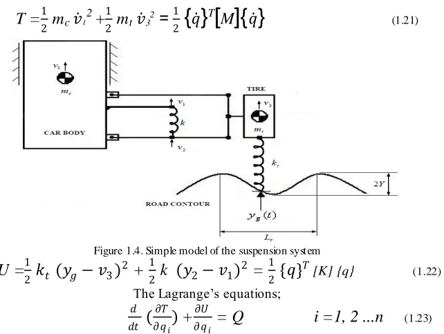
Double wishbone suspension of a quarter cars is modelled assuming the suspension links to be rigid. The model is shown in Figure 3.3.The mass t m represents approximately the mass of the wheel plus part of the mass of the suspension arms, c m represents approximately 1/4 of the car mass.
Figure 1.3. Simple model of thesuspension system
Simple Modelling Of Suspe nsion Syste m
Double wishbone suspension of a quarter cars is modelled assuming the suspension links to be rigid. The model is shown in Figure 1.4. The mass t m represents approximately the mass of the whee l p lus part of the mass of the
suspension arms; mc represents approximate ly 1/4 o f the car mass. The e xcitation co mes fro m the road irregularity. It is
considered that the spring is located in the middle of the lo wer control a rm. The kinetic and strain energies as;
T =
12
m
c𝑣 1
2
+
1 2m
t𝑣
32
=
12
{
𝑞
}
T
[
M
]
{
𝑞
}
(1.21)Figure 1.4. Simple model of the suspension system
U =
12
𝑘
𝑡(𝑦
𝑔− 𝑣
3)
2
+
12
k
(𝑦
2− 𝑣
1)
2
=
12
{𝑞}
𝑇
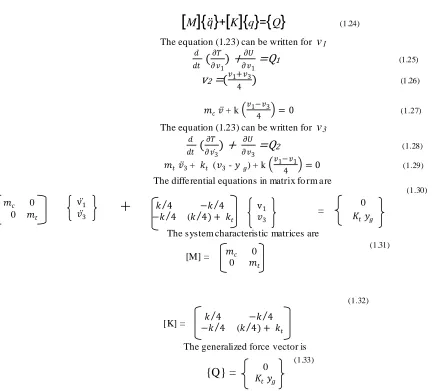
[K] {q} (1.22) The Lagrange’s equations;
𝑑
𝑑𝑡
(
𝜕𝑇 𝜕𝑞𝑖
)
+
𝜕𝑈
𝜕𝑞𝑖
= Q i =1, 2 ...n
(1.23)Where the total strain energy U = 𝑈𝑒 +𝑈𝑔 , and 𝑄𝑖 are genera lised forces. The Lagrange’s equations (1.23) y ield the
[
M
]
{
𝑞
}
+
[
K
]
{
q
}
=
{
Q
}
(1.24)The equation (1.23) can be written for
v
1𝑑 𝑑𝑡
(
𝜕𝑇
𝜕𝑣1
) +
𝜕𝑈
𝜕𝑣1
=Q
1(1.25)
v
2=(
𝑣1+𝑣34
)
(1.26)𝑚𝑐 𝑣 + k
𝑣1−𝑣3
4 = 0 (1.27)
The equation (1.23) can be written for
v
3𝑑 𝑑𝑡
(
𝜕𝑇 𝜕𝑣3
) +
𝜕𝑈
𝜕𝑣3
=Q
2 (1.28)𝑚𝑡 𝑣 3 + 𝑘𝑡 (𝑣3 - 𝑦 𝑔) + k
𝑣1−𝑣1
4 = 0 (1.29) The diffe rential equations in matrix fo rm a re
(1.30)
+
=The system characteristic matrices are
(1.31)
[M] =
(1.32)
[K] =
The generalized force vector is
(1.33)
{Q} =
On the other hand, Equation (3.30) represents a mathe matica l model shown in Figure 1.4.If the base displacement is
defined by a single frequency harmonic of the form as, yg (t) = Y Sin we t.
Figure 1.4. A quarter car suspension model (Source:Gobbi and Mastinug)
𝑚𝑐 0
0 𝑚𝑡
v1
𝑣3
𝑘 4 −𝑘 4
−𝑘 4 (𝑘 4)+ 𝑘𝑡
v1
𝑣3
0 𝐾𝑡𝑦𝑔
𝑚𝑐 0
0 𝑚𝑡
𝑘 4 −𝑘 4
−𝑘 4 (𝑘 4)+ 𝑘𝑡
The frequency of base motion is we
𝑤
𝑒=
2 𝜋 𝑉𝐿𝑟
(1.34)
Where V is the vehicle speed and Lr is the period of the road profile.
Finite Ele me nt Modelling Of Suspe nsion Syste m
Figure 1.5. Finite element model of the suspension system
The lowe r and the upper a rms are div ided into two ele ments, as shown in Figure 1.5. The degrees of freedo m of node i
are ui, vi and θi. The degree of freedo m v i is transverse displacement and ui is a xia l displace ment and θi is slope or
rotation.
The global displace ment vector
{
q
}= {
u
1,v
1,θ
1,u
2,v
2,θ
2,u
3,v
3,θ
3,u
4,θ
4,u
5,v
5, θ
5,θ
6,θ
7}
𝑇(1.35) The local degrees of freedom for a single e le ment are represented by Equation (1.1);
{
q
}={
u
1,v
1,θ
1,u
2,v
2,θ
2,}
T(1.35)
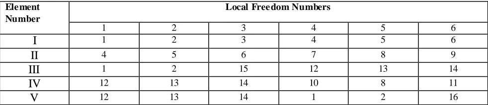
The connectivity table for the e le ment solution is given in Tab le 1.1. Every node in an ele ment has both a local coordinate and a global coordinate. The elastic stiffness, geometric stiffness, mass matrices are found fro m Equations (1.6), (1.8), and (1.10) for each the plane fra me e le ment. The global stiffness, geometric , and mass matrices are obtained by assembling these element matrices. The spring ele ment given in Equation (1.12) is considered a fra me ele ment.
Ele ment Number
Local Free dom Numbers
1 2 3 4 5 6
I
1 2 3 4 5 6II
4 5 6 7 8 9III
1 2 15 12 13 14IV
12 13 14 10 8 11V
12 13 14 1 2 16X.CONCLUS ION
The quarter car with the double wishbone suspension system has been modelled for two d ifferent approaches to the suspension links to be rig id and fle xib le. There fore, the dynamic analyses of these models have been investigated by
the finite e le ment method
.
Analysis of the results showed that the agreement between the simp le model and fle xib lemodel without unloaded lin ks is e xcellent for both natural frequencies and the time responses. Therefore, the simp le model is adequate for the first design step. However, in order to obtain the more accurate results, for e xa mple natural
frequencies and time responses, it is necessary to consider the fin ite ele ment model of the suspension system
.
REFERENCES
1] Chandrupatla, T.R. and Belegundu, “ Beams and Frames”, in Introduction to Finite Elements in Engineering, (Prentice-Hall Inc., Upper Saddle River), p.238.
2] Chopra, A.K., “ Damping in structures”, in Dynamics of Structures, (Prentice-Hall Inc., Upper Saddle River, New Jersey), pp.409-429.
3] Cook, R.D., Malkus, D.S. and Plesha, “ Stress Stiffening and Buckling”, in Concepts and Applications of Finite Element Analysis, (John Wiley&Sons,NewYork), pp.429-448.
4] Gillespie, T .D. “ Suspensions”, in Fundamentals of Vehicle Dynamics, (Society of Automotive Engineers, USA), pp.97-117 and pp.237-247. 5] Gobbi M. and Mastinug G.“ Analytical Description and Optimization of the Dynamic Behaviour of Passively Suspended Road Vehicles”, Journal of Sound and Vibration, 245(3), pp.457-481.
6] Kwon, Y.W. and Bang, H.“ Beam and Frame Structures”, in The Finite ElementMethod using Matlab, (CRC Press Inc, USA), pp.259-264.41 7] Milliken, W.F. and Milliken, D.L., 1995. “ Historical Note On Vehicle Dynamics Development” and “ Suspension Geometry”, in Race Car Vehicle Dynamics, (Society of Automotive Engineers, USA), pp.413-607.
8] Petyt, M. “Forced Response 1 and Forced Response 2”, in Introduction to FiniteElement Vibration Analysis, (The Bath Press, Great Britain), pp.386-450.