Scholarship at UWindsor
Scholarship at UWindsor
Electronic Theses and Dissertations Theses, Dissertations, and Major Papers
2008
Protocol-level performance analysis and implementation for
Protocol-level performance analysis and implementation for
anti-collision protocols in RFID systems
collision protocols in RFID systems
Mohammed Berhea
University of Windsor
Follow this and additional works at: https://scholar.uwindsor.ca/etd
Recommended Citation Recommended Citation
Berhea, Mohammed, "Protocol-level performance analysis and implementation for anti-collision protocols in RFID systems" (2008). Electronic Theses and Dissertations. 8233.
https://scholar.uwindsor.ca/etd/8233
Implementation for Anti-Collision Protocols in
RFID Systems
by
Mohammed Berhea
A Thesis
Submitted to the Faculty of Graduate Studies through the
Department of Electrical and Computer Engineering in Partial Fulfillment of the Requirements for the Degree of Master of Applied Science at
The University of Windsor
Windsor, Ontario, Canada 2008
1*1
Published Heritage Branch
395 Wellington Street Ottawa ON K1A0N4 Canada
Direction du
Patrimoine de I'edition
395, rue Wellington Ottawa ON K1A0N4 Canada
Your file Votre reference ISBN: 978-0-494-47025-1 Our file Notre reference ISBN: 978-0-494-47025-1
NOTICE:
The author has granted a non-exclusive license allowing Library and Archives Canada to reproduce, publish, archive, preserve, conserve, communicate to the public by
telecommunication or on the Internet, loan, distribute and sell theses
worldwide, for commercial or non-commercial purposes, in microform, paper, electronic and/or any other formats.
AVIS:
L'auteur a accorde une licence non exclusive permettant a la Bibliotheque et Archives Canada de reproduire, publier, archiver,
sauvegarder, conserver, transmettre au public par telecommunication ou par Plntemet, prefer, distribuer et vendre des theses partout dans le monde, a des fins commerciales ou autres, sur support microforme, papier, electronique et/ou autres formats.
The author retains copyright ownership and moral rights in this thesis. Neither the thesis nor substantial extracts from it may be printed or otherwise reproduced without the author's permission.
L'auteur conserve la propriete du droit d'auteur et des droits moraux qui protege cette these. Ni la these ni des extraits substantiels de celle-ci ne doivent etre imprimes ou autrement reproduits sans son autorisation.
In compliance with the Canadian Privacy Act some supporting forms may have been removed from this thesis.
Conformement a la loi canadienne sur la protection de la vie privee, quelques formulaires secondaires ont ete enleves de cette these.
While these forms may be included in the document page count,
their removal does not represent any loss of content from the thesis.
Bien que ces formulaires
Publication
I. Co-Authorship Declaration
I hereby declare that this thesis incorporates material that is result of joint research, as follows:
In all cases, the primary contributions, derivations, experimental setups, data analysis and interpretation were performed by the author through the supervision of Dr. C. Chen. In addition to supervision, Dr. C. Chen provided the author with the project idea, guidance, and financial help. Dr. C. Chen had also held regular meetings with Dr. Q. M. Jonathan Wu regarding project discussions and follow-ups about the progress and outcome of this project.
I am aware of the University of Windsor Senate Policy on Authorship and I certify that I have properly acknowledged the contribution of other researchers to my thesis, and have obtained written permission from each of the co-author(s) to include their contributions in my thesis.
This thesis includes 2 original papers that have been previously published / submitted for publication in peer reviewed journals, as follows:
Thesis Chapter
Chapter 3, 4, and 5
Chapter 3, 4, 5, and 6
Publication title/full citation
M. Berhea, C. Chen, and Q. M. J. Wu, "Protocol-Level Performance Analysis for Anti-Collision Protocols in RFTD Systems", In Proceedings of 2008 IEEE International Symposium on Circuits and Systems (ISCAS'08), May 2008, Seattle, USA
M. Berhea, C. Chen, and Q. M. J. Wu, "Protocol-Level Performance Analysis and Implementation for Anti-Collision Protocols in RFID Systems"
Publication status*
"Accepted for poster session "
"Submitted for publication" to IEEE Trans. On Vehicular Technology
I certify that I have obtained a written permission from the copyright owner(s) to include the above published material(s) in my thesis. I certify that the above material describes work completed during my registration as graduate student at the University of Windsor.
I would like to express my sincere appreciation to my supervisor Dr. Chunhong Chen for his guidance and encouragement. He introduced me to this interesting research area and guided me throughout my thesis with great patience. I would like to thank the members of my thesis committee, Dr. Behnam Shahrrava and Dr. Dan Wu for their advice regarding the research process and their assistance in the preparation of this thesis. Here, I would also like to thank Dr. Rashid Rashidzadeh and Dr. Roberto Muscedere for their incessant help during my chip design.
DECLARATION OF CO-AUTHORSHIP / PREVIOUS PUBLICATION Ill
I. Co-AUTHORSHIP DECLARATION m
II. DECLARATION OF PREVIOUS PUBLICATION iv
ABSTRACT VI ACKNOWLEDGEMENTS VII
LIST OF FIGURES XII LIST OF TABLES XIV CHAPTER 1 INTRODUCTION 1
1.1. RFID SYSTEM 1
1.2. OBJECT IDENTIFICATION AND ANTI-COLLISION PROTOCOLS 2
1.3. MOTIVATION AND ACHIEVEMENTS 6
1.4. THESIS ORGANIZATION 7
CHAPTER 2 REVIEW OF ANTI-COLLISION PROTOCOLS 8
2.1. COST FUNCTION FOR ANTI-COLLISION PROTOCOLS 8
2.2. BINARY-TREE PROTOCOL 11 2.3. QUERY-TREE PROTOCOL 12
2.4. IMPROVED QUERY-TREE PROTOCOL 14 2.5. COMPARISON OF THE THREE PROTOCOLS 15
CHAPTER 3 PROTOCOL-LEVEL ANALYSIS OF TREE-BASED
3.1.1. Determination of worst-case scenario 20
3.1.2. Derivations of protocol-level performance metrics for Binary-Tree Protocol.
22
3.2. PROTOCOL-LEVEL ANALYSIS OF QUERY-TREE PROTOCOL 27 3.3. PROTOCOL-LEVEL ANALYSIS OF IMPROVED QUERY-TREE PROTOCOL 33
CHAPTER 4 A COMBINED BINARY-QUERY-TREE PROTOCOLTHE
PROPOSED PROTOCOL 39
CHAPTER 5 PROTOCOL-LEVEL COMPARISON OF THE FOUR TREE
PROTOCOLS 46
5.1. PROTOCOL-LEVEL COMPARISON OF THE BINARY, QUERY, AND IMPROVED QUERY
TREE PROTOCOLS 46 5.2. PROTOCOL-LEVEL COMPARISON OF THE PROPOSED PROTOCOL WITH BINARY
AND IMPROVED QUERY PROTOCOLS 50 CHAPTER 6 IMPLEMENTATION AND COMPARISON OF THE FOUR
PROTOCOLS AT DIFFERENT LEVELS OF ABSTRACTION 52
6.1. IMPLEMENTATION AND SIMULATION OF THE BINARY-TREE PROTOCOL 53 6.2. IMPLEMENTATION AND SIMULATION OF THE QUERY-TREE PROTOCOL 55
6.3. IMPLEMENTATION AND SIMULATION OF THE IMPROVED QUERY-TREE PROTOCOL 57 6.4. IMPLEMENTATION AND SIMULATION OF THE COMBINED-BINARY-TREE
PROTOCOL 59 6.5. LAYOUT LEVEL COMPARISON OF THE FOUR PROTOCOLS 61
6.5.1. Comparison of the four protocols using "Encounter" 61
6.5.2.2. Results from Physical Implementation for Query-Tree Protocol 68 6.5.2.3. Results from Physical Implementation for Improved Query-Tree
Protocol 71 6.5.2.4. Results from Physical Implementation for Combined-Binary-Tree
Protocol 74
CHAPTER 7 CONCLUSIONS AND FUTURE WORK 77
7.1. CONCLUSIONS AND CONTRIBUTIONS 77
7.2. FUTURE WORK 78
REFERENCES 79 APPENDIX A RTL CODES AND TEST BENCHES 82
A.l. RTL CODE AND TEST BENCH FOR THE BINARY-TREE PROTOCOL 83
A.l.l. RTL Code for the Binary-Tree Protocol 83
A.1.2. Test bench for the Binary-Tree Protocol 86
A.2. RTL CODE AND TEST BENCH FOR THE QUERY-TREE PROTOCOL 88
A.2.1. RTL Code for the Query-Tree Protocol 88
A.2.2. Test bench for the Query-Tree Protocol 91
A.3. RTL CODE AND TEST BENCH FOR THE IMPROVED QUERY-TREE PROTOCOL 94
A.3.1. RTL Code for the Improved Query-Tree Protocol 94
A.3.2. Test bench for Improved Query-Tree Protocol 97
A.4. RTL CODE AND TEST BENCH FOR THE QUERY-TREE PROTOCOL 100
A.4.1. RTL Code for the Proposed Protocol 100
A.4.2. Test bench for the Proposed Protocol 104
COMBINED-BINARY PROTOCOLS 114
APPENDIX C PERMISSION FROM CO-AUTHORS AND IEEE 121
C.l. PERMISSION TO USE PREVIOUSLY SUBMITTED/ACCEPTED PAPERS 122
C.2. PERMISSION TO REUSE IEEE-COPYRIGHTED MATERIAL 123
Figure 1.1: Typical RFID system 1 Figure 1.2: Collision Resolution Protocols 3
Figure 1.3: Example of Binary-Tree algorithm 5 Figure 1.4: Example of Query-Tree algorithm 5 Figure 2.1: Rectification Circuit in a practical tag 9 Figure 2.2: State diagram for Binary-Tree Protocol 11 Figure 2.3: State diagram for Query-Tree Protocol 13 Figure 4.1: State diagram for the Combined-Binary-Query-Tree Protocol 39
Figure 5.1: Performance comparison of binary-tree, query-tree and
improved-query-tree protocols under their worst cases (n = 4) 48 Figure 5.2: Performance comparison of binary-tree, query-tree and
improved-query-tree protocols under their worst cases (n = 8) 49 Figure 5.3: Performance comparison of binary-tree, improved query-tree and
combined binary-query-tree protocols under their worst cases (n = 4) 51 Figure 6.1: Simulation output for Tag # 15 (N = 4, n = 4): Binary-Tree Protocol... 53
Figure 6.2: Schematic for Tag # 15 (N = 4): Binary-Tree Protocol 54 Figure 6.3: Layout for Tag # 15 (N = 4): Binary-Tree Protocol 55 Figure 6.4: Simulation output for Tag# 15 (N = 4, n = 4): Query-Tree Protocol 56
Figure 6.9: Layout for Tag# 15 (N = 4): Improved-Query-Tree Protocol 59 Figure 6.10: Simulation output for Tag# 15 (N = 4, n = 4): Combined-Query-Tree
Protocol 60 Figure 6.11: Schematic for Tag# 15 (N = 4): Combined -Query-Tree Protocol 60
Figure 6.12: Layout for Tag# 15 (N = 4): Combined -Query-Tree Protocol 61 Figure 6.13: Test setup to determine instantaneous power by Binary-Tree Protocol
(N = 4, n = 2) 66 Figure 6.14: Results of Simulation for Binary-Tree Protocol (N = 4, n = 2) 67
Figure 6.15: Instantaneous power for Binary-Tree Protocol (N = 4, n = 2) 68 Figure 6.16 Results of Simulation for Query-Tree Protocol (N = 4, n = 2) 70 Figure 6.17: Instantaneous power for Query-Tree Protocol (N = 4, n = 2) 71 Figure 6.18: Results of Simulation for Improved Query-Tree Protocol (N = 4, n = 2)
72 Figure 6.19: Instantaneous power for Improved Query-Tree Protocol (N = 4, n = 2)
73 Figure 6.20: Results of Simulation for Combined-Binary-Query-Tree Protocol (N =
4, n = 2) 75 Figure 6.21: Instantaneous power for Combined-Binary-Query-Tree Protocol (N = 4,
Table 2.1: The inquiry process of Binary-Tree protocol on a 3-tag example 12 Table 2.2: The inquiry process of Query-Tree protocol on a 4-tag example 13 Table 2.3: The inquiry process of improved query-tree protocol on a 4-tag example
14 Table 3.1: Identification Process of Two Tags by Binary-Tree Protocol for N = 4 . 17 Table 3.2: Identification Process of Two Tags (Tag# 10, Tag# 12) by Binary-Tree
Protocol for N = 4 18 Table 3.3: Identification Process of Five Tags by Binary-Tree Protocol for N = 4 . 19
Table 3.4: Distribution of Tags with Binary-Tree Protocol for Worst-Case Scenario 21 Table 3.5: Identification Process of Two Tags by Query-Tree Protocol for N = 5.. 28 Table 3.6: Commands used for Query-Tree Protocol with corresponding # of
transitions and # of clock cycles for N = 4 and N = 5 29 Table 3.7: Identification Process of Two Tags by Improved Query-Tree Protocol for
N = 5 34 Table 3.8: Identification Process of Four Tags by Improved Query-Tree Protocol for
N = 5 36 Table 4.1: Identification Process of Two Tags by Combined Binary-Query-Tree
Protocol for N = 5 40 Table 4.2: Identification Process of Four Tags by Combined Binary-Query-Tree
binary-tree has lower power consumption over the two query-tree types 48
Table 6.1: Mapping of Outl and Out2 to the tag response 52 Table 6.2: Capacitance information for the Binary-Tree Protocol 64
Table 6.3: Implementation results for the Binary, Query, Improved-Query, and
1.1. RFID System
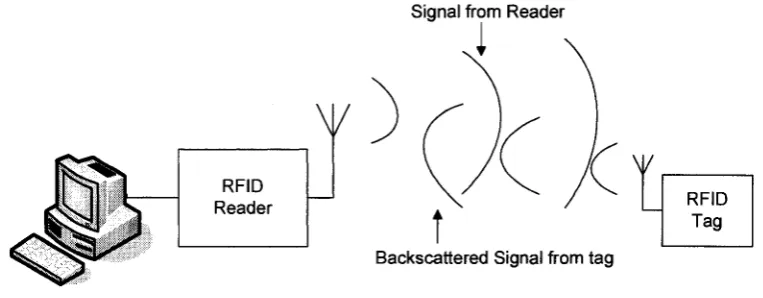
Radio Frequency Identification (RFID) system is an automatic identification system that uses radio frequency to identify objects. The system is consisted of a reader, a tag, and a host computer as shown in Figure 1.1. RFID reader identifies objects through wireless communications with tags which have unique ID and information, and are attached to objects.
Signal from Reader
i
v
Backscattered Signal from tag
Figure 1.1: Typical RFID system
In passive RFED, the reader is designed to transmit energy to, and read information from the tags. The tag is composed of an antenna and a silicon chip that includes basic modulation circuitry and non-volatile memory that permanently stores its ID number [1, 2]. The tag is energized by a time-varying electromagnetic radio frequency (RF) wave that is transmitted by the reader. The RF field generated by a tag reader has three purposes: induce enough power into the tag coil to energize the tag, provide a synchronized clock source to the tag, and to act as a carrier for return data from the tag.
1.2. Object Identification and Anti-Collision Protocols
A passive tag is power limited, rather than energy limited. We can reasonably assume that the reader can always keep the energy supply so that a problem such as battery life doesn't exist [1, 13]. Moreover, the available power from the reader field, not only reduces very rapidly with distance, but is also controlled by strict regulations, resulting in a limited communication distance of 4 - 5m when using the UHF frequency band (860 MHz - 930 MHz) [14]. Thus the key focusing point in this thesis is to concentrate on the way of reducing the tag's power consumption, which restricts the tag's maximum possible distance to the reader.
consumption through assessing different anti-collision protocols is critical in implementation of the tags which depend on the protocols they use within the system.
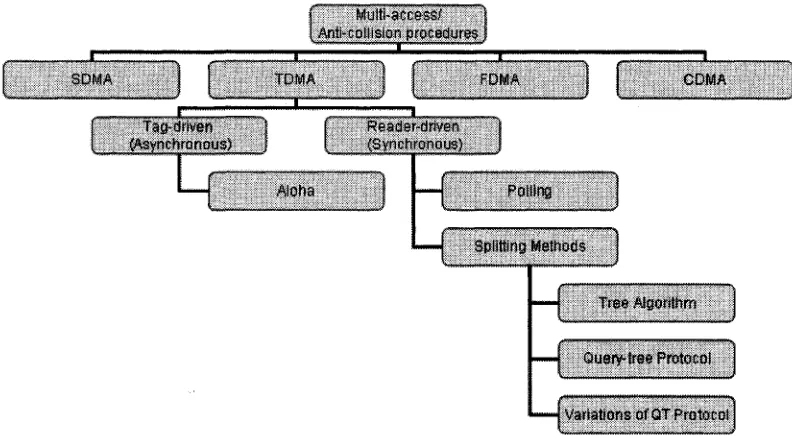
In order to resolve collisions, numerous procedures have been developed with the objective of separating the individual participant signals from one another Basically, there are four different procedures [3, 9]: space division multiple access (SDMA), frequency domain multiple access (FDMA), time domain multiple access (TDMA), and code division multiple access (CDMA) as shown in Figure 1.2[9]. SDMA and FDMA are expensive for implementation and are restricted to a few specialized applications while CDMA needs complex circuits and generally rejected for RFID use.
Multi-access/ Anti-collision procedures j
SDMA
3C TDMA
X 3„
FDMA COMA
Tag-driven (Asynchtonous)
Reader-driven (Synchronous)
Aloha Polling
Splitting Methods
Variations of QT Protocol
Figure 1.2: Collision Resolution Protocols
nature and simple, thus enabling simpler reader and tag implementations. However, they are subject to tag starvation problem, a serious situation where it might either take a long time, or be unable, to identify a tag [7, 8]. In contrast, the tree-based search protocols [4, 5, 15] are deterministic in nature. They are able to read all tags by successively querying nodes at different levels of the tree, with tag IDs distributed on the tree based on their prefix. The guarantee that all tags IDs will be read within a certain time frame has made the tree-based search protocol desirable in many applications. The tree search procedure, however, uses up a lot of reader queries and tag responses by relying on colliding responses of tags to determine which sub-tree to query next. This results in higher energy consumption at the readers and tags (if they are active tags).
0.
,v 1. R
R L :••) ( BR
0
(g)
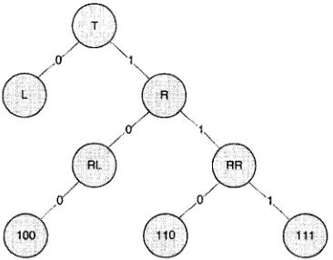
Figure 1.3: Example of Binary-Tree algorithm
\
00 01 10 11
V
000 001
• •
Figure 1.4: Example of Query-Tree algorithm
1.3. Motivation and Achievements
Previous work (such as [1]) on low power implementation for tree-based protocols was done at circuit-level where a particular protocol could be implemented in different ways with totally different power consumption, leading to an unfair performance evaluation and comparison among various protocols. This work is to assess different performance metrics such as number of transitions, clock cycles, energy, and power consumption of tree-based protocols at protocol-level which is independent of circuit implementation and more efficient.
The basic idea is for a particular N (number of bits that represent and ID) and n (number tags that simultaneous exit for identification) to look at the state diagram for each protocol and to find out the number of state transitions and clock cycles required (and hence its power and energy consumption) before all tags are identified. A general equation for the number of transitions and clock cycles as a function of N and n is then formulated. Then energy consumption which is proportional to the ratio of number of state transitions to number of clock cycles and power consumption which is directly proportional to number of state transitions under equal inquiry time for all protocols were determined. An improved protocol that combines the binary-tree and query-tree is also proposed for further performance improvement.
Accurate power then was estimated at the layout level based on the switching activity and the total capacitance.
1.4. Thesis Organization
This thesis is organized as follows.
In Chapter 2 we describe the previous work [1] that deals with circuit-level optimization of power consumption of tags using tree-based protocols. In Chapter 3, for the tree-based protocols mentioned in Chaper2, our analysis will be based on protocol-level instead of circuit-level. For a typical Binary-Tree Protocol case, the number of transitions and clock cycles are tabulated. For this protocol, the condition for the worst case scenario is determined and formula that will allow us to calculate the number of transitions and clock cycles for any ID bits and number of tags is formulated. This chapter also shows similar analysis for Query-Tree and Improved Query-Tree protocols respectively.
Chapter 4 introduces the work of the proposed protocol, Combined Binary-Query-Tree Protocol. In Chapter 5 protocol-level performance evaluation criterion is developed and the three protocols mentioned in Chapter 2 are compared in terms of total number of transitions, total number of clock cycles, energy, and power consumption before a tag is fully read by a reader. Chapter 5 also compares the proposed protocol with binary and improved-query protocols at protocol-level.
This chapter summarizes the work done in [1] that this thesis work is related to.
In the design of RFID tags, the main objective is to reduce power consumption within a tag so as to maximize the working distance between the reader and the tag. Since an anti-collision protocol circuit is the main part of a tag, selecting and implementing a suitable protocol from a low-power consumption point of view, will be a key design criteria. Hence, it is necessary to develop a cost function that can measure the maximum instant power consumption of the circuit [1],
2.1. Cost Function for Anti-Collision Protocols
In the design of RFID tags, the main objective is to reduce power consumption within a tag so as to maximize the working distance between the reader and the tag. Since an anti-collision protocol circuit is the main part of a tag, selecting and implementing a suitable protocol from a low-power consumption point of view, will be a key design criteria. Hence, it is necessary to develop a cost function that can measure the maximum instant power consumption of the circuit.
In passive RFID systems, the electromagnetic power a tag can receive from the reader is given by (2.1) [1,3]:
Where, P = AS and A = ^ - S = - ^ %
p =A2PG,G, Am1
(2.1)
Where,
S = radiation density, PEIRP = Effective Isotropic Radiated Power, Pe = Power received by tag, P = power injected into reader's antenna, r = distance between reader and tag, Gs = gain of reader's antenna, Gr = gain of tag's antenna, X = wave length of the emitted electro-magnetic wave
Figure 2.1 shows the rectification circuit of a practical tag. When received input power is lower than instantaneous power consumption, the capacitor (C) will provide the required energy compensation. On the other hand, when input power is higher than instantaneous power consumption, transistor (Ml) will be turned on to bypass the extra current so as to keep the operating voltage at
Vdd-±CV2dd ~\c{Vdd -AVf=EhJ2 -Pin(t2 -tl)T (2.2)
Therefore, for any period of time (ti, t2) (measured in clock cycles), conservation of energy will lead us to the following equation:
Where,
AV is the change in capacitance voltage (Vdd), Pin is the input power, Eti,t2 is the total energy consumed within the period ti to t2.
With the maximum acceptable voltage drop of Vdr0p, and assuming AV « Vdd, Pin is simplified to be:
P,. >•
V2dd-C, load ( u
ih-h)r
IA-cv.
dropV h * dd ' (-load J
(2.3)
Where A; is number of 0 to 1 transitions within clock cycle i and Qoad is the load capacitance of the circuit.
Hence, for any arbitrary anti-collision protocol,
Pin^^MaxiP^t^t^eT.}
(2.4)Where P (ti, i*i) represents the right-hand equation of (2.3) and Tinq is the total inquiry time for a tag to be totally read by the reader. Pin,min, the lower bound for input power of tags, is defined as the cost function used to evaluate different protocols.
For fair power consumption comparison among different protocols, equal inquiry time
(TINQ) for all protocols need to be considered. Hence, with TINQ = T • Cyc, where Cyc is
total number of clock cycles needed to fully read a tag, P(ti, t2) will be adjusted to the following equation:
P(t2,t1) =
Cyc-V2dd-Ci load
k-'ift
i r INQCyc r
('
2-0
*2
1 4
-V='i
Z 4
-cv ^
^ y drop
V C
vdd ^load J
cv,
drop * dd ' ^load J(2.5)
2.2. Binary-Tree Protocol
Binary-Tree Protocol enables a reader to successfully read all tags within its reach by using binary search algorithm [1,9]. The tags are assumed to have an ID-bit module, and the reader sends one bit at a time during the enquiry. The tags with the same received bit progressively increment their bit position to send the next bit in their ID. If the tags receive a different inquiring bit, they will go to the state of "standby" and stay there until a tag is identified (or killed) with the rest of the tags being reset. During an enquiry, the reader sends '0' when it senses a collision. Otherwise, it uses the received bit from the tag as the next inquiring bit.
The state diagram used by the tag for this protocol is shown in Figure 2.2 [1]
Not the Same Last bit bit
State assignment SO
S1 S2 S3
Standby Receiving Sending Killed
Figure 2.2: State diagram for Binary-Tree Protocol
An example shown in Table 2.1 [1] details what steps a reader need to use to fully identify three tags if the tags are using Binary-Tree Protocol. In the table, under "Tags answer" column, * stands for collision situation and empty space represents no-response situation.
COST, = [ 2 * ( » - l ) + 3 ]
f
Where, R =
1 10
V 2 n - l R
CV drop C V
(2-6)
(2.7)
Here "n" represents the length of the ID, and "k" represents the distribution of tags (total number of tags simultaneously available for interrogation.
Table 2.1: The inquiry process of Binary-Tree protocol on a 3-tag example
Reader sends
0 0 0 1 0 1 0
Tags answer
* 1 1 1
0 0
Identified tag
(remaining tags reset)
001
Oil
100
2.3. Query-Tree Protocol
The state diagram used by the tag for this protocol is shown in Figure 2.3 [1]
Same Start Prefi:
Not sami
Finished Sending
State assignment
Finished receiving
SO S1 S2
Standby Receiving Sending
Send remaining bits
Figure 2.3: State diagram for Query-Tree Protocol
An example elaborating the process of identification of four tags (with 4-bit ID) that uses Query-Tree protocol is shown in Table 2.2 [1].
Table 2.2: The inquiry process of Query-Tree protocol on a 4-tag example
Reader sends
start 0 000 001 1 10 11
Tags answer
##**
0*1 1 1 *00
00 00
Identified tag
(remaining tags reset)
0001 0011
1000 1100
Also, after implementing this protocol and analyzing its cost function, the following formula is derived [1]:
COSTquery=[k{2n + S)-{n + 3)]
Where,m = [log k\
8 — m — 9m + 4
l{n + A\m + l)+A (n + 4)(m + l) + 2 R (2.8)
2.4. Improved Query-Tree Protocol
This protocol is similar to the query-tree protocol, the difference lies on the action that will be taken by the reader when it senses collision. In case of query-tree, tags will continue to send the remaining of their ID bits, even though there is a collision. On the other hand, in Improved Query-Tree-Protocol, when the reader senses a collision, it issues a 'Stop Send" command ("SS") to all the tags to halt transmission. This process will then reduce unnecessary "sending" operations by the tags and effectively reducing power consumption.
The state diagram for this protocol is similar to Figure 2.3 except that the "Finished Sending" edge should be replaced by "Stop Sending" edge.
The Improved query-tree search process in identification of the same four tags that were used in Table 2.2 is shown in Table 2.3 [1]:
Table 2.3: The inquiry process of improved query-tree protocol on a 4-tag example
Reader sends
start 0 000 001 1 10 11
Tags answer
* 0*
1 1 * 00 00
Identified tag (remaining tags reset)
0001 0011
1000 1100
After implementing this protocol, the following formula is derived for its cost function [1]:
COSTim,=[k{n + m + B)-3] 8 - m2- 3 3 m - 2 6 - 2 f l 2n + m2 + llra + 12
(2.10)
2.5. Comparison of the three protocols
After drawing curves using the cost functions developed in equations (2.6), (2.8), and (2.10), the following general information is deduced [1]:
• With increase in n, the probability of the Query-Tree protocol outperforming the Binary-Tree protocol in terms of power consumption is better. Especially, with small values of R, the performance of Query-Tree protocol as compared to the Binary-Tree protocol is significant.
• Since Improved Query-Tree protocol is always better than Query-Tree protocol, whatever observation made between the Query-Tree protocol and the Binary-Tree protocol holds true when comparing Improved Query-Tree protocol with Binary-tree protocol with added performance in case of Improved query-tree protocol.
By omitting the low power items [13] shows that:
For R < 14.4n - 274.2, COST improved < COST binary For R < 4n - 75, COST queiy < COST binary
Tree-based Anti-Collision Protocols
In this chapter analysis of the three tree-based protocols that were discussed in Chapter 2 will be performed at the protocol level. As mentioned in Chapter 1 and shown in Chapter 2, the previous work was concentrated on the determination of instant power consumption of circuits for comparison of different tree-based anti-collision protocols. But a particular protocol could be implemented in different ways bringing about different power consumptions hence; performance evaluation and comparison among various protocols need to be done at protocol level. Therefore, in this work protocol-level performance metrics such as number of transitions, clock cycles, energy, and power consumption will be used to compare different tree-based protocols.
3.1. Protocol-Level Analysis of Binary-Tree Protocol and
determination of worst-case scenario
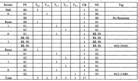
In general, the tag identification process can be shown in details based on Figure 2.2 (State diagram for Binary-Tree Protocol). Table 3.1 shows an example for N = 4 with 2 tags present. In this table, the 1st column represents the command sent by the reader, the 2nd column is the present state (PS) of the tag, and the following five columns show the number of transitions, Ty, that the tag makes from state S; to state Sj. The Clk column in the table denotes the number of clock cycles required, while the NS column indicates the next state. The status of tags that are interacting with the reader is shown in the last tag column, where the two tags #12 (representing ID#1100) and #14 (representing ID#1110) are shown to be read at the 10 and 17 clock cycle, respectively.
Table 3.1: Identification Process of Two Tags by Binary-Tree Protocol for N = 4
Reader Null 0 Reset 1 1 0 Reset 1 1 1 Total PS SO SI SO SO SI S2 SI S2 SI S2.S0 SO SI S2 SI S2 SI S2 -To-i 1 1 1 3 Ti-o 1 1 2 Tl-2 1 1 1 1 1 5
T2-i
1 1 1 1 4 T2.3 1 1 Clk 17 NS SI SO so si S2 SI S2 SI S2. SO S3. SO SI S2 SI S2 SI S2 S3 -Tag No Response #12 0100) #14(1110)
states are written to indicate the states of Tag# 12 and Tag# 14, where the state with the bold font representing the state of Tag# 12. Once Tag #12 is identified (after the 10th clock cycle), the state transitions shown in the table are made by Tag# 14. It takes 15 numbers of transitions for Tag# 14 to be identified.
Table 3.2: Reader Null 0 Reset 1 0 1 Reset 1 1 0 Total
Identification Process of Two Tags (Tag# 10, Tag# 12) by Binary-Tree Protocol for N = 4
PS SO SI so so SI S2 SI S2. SO SI. SO S2.S0 SO SI S2 SI S2 SI S2 -To-, 1 1 1 3 TLO 1 1 Tl-2 1 1 1 1 1 5
T2-i
1 1 1 3 T2-3 1 1 Clk 17 NS SI SO SO SI S2 SI S2. SO SI. SO S2.S0 S3. SO SI S2 SI S2 SI S2 S3 -Tag No Resoonse #10(1010) #12 (1100)
-For comparison, we draw a table, Table 3.2 that shows the reading process if the two tags are Tag# 10 and Tag# 12. From Table 3.2, the total number of transitions that Tag# 12 makes before it is read is 13, which is lower than 15 compared to the result obtained from Table 3.1. In fact, if we consider any combinations of two tags, the total number of transitions that we can obtain will always be lower than the combination shown in Table
3.1. H e n c e , for any t w o tags to b e identified with this protocol, the highest possible
number of state transitions occurs when the ID of one tag is 1110 (Tag# 14) or 1111 (Tag# 15) and the ID of the other is 1100 (Tag# 12) or 1101(Tag# 13). This is called the
worst-case scenario. Note that if Tag# 14 (1110) and Tag# 15 (1111) simultaneously
reading the last bit. If the last bit is 0, then it is Tag# 14; if the last bit is 1, then it is Tag# 15; if the expected last bit turned out to be a collision, then both Tag# 14 and Tag# 15 are present.
Table 3.3: Identification Process of Five Tags by Binary-Tree Protocol for N = 4
3.1.1. Determination of worst-case scenario
In order to find out the worst-case scenario for any value of N with a given number of tags, we analyze the number of state transitions and clock cycles required for different tags i N bits in their ID, and summarize the results in Table 3.4 which can be used to determine the ID distribution of the tags that yield a worst-case scenario. In this table, the tags whose most significant bits match in a particular pattern are listed in a group. For example, for a tag represented with a 4-bit ID, Tag# 14 (ID of 1110) and Tag# 15 (ID of 1111) belong to the same group (group # 4) or Tag# 8 (1000), Tag# 9 (1001), Tag# 10 (1010), and Tag# 11 (1011), belong to the same group (group # 2) as shown in Table 3.4.
From Table 3.1 we can see that after Tag# 12 is read, Tag# 14 (or Tag# 15) takes 7 numbers of transitions before it is read (that is, by counting the number of transitions it makes from SO to S3). This same tag (Tag# 14) took 6 number of transitions while Tag# 12 is being read (that is from the 4th clock cycle up to the 10th clock cycle in Table 3.1). If we see Table 3.3, Tag# 14 will take 4 numbers of transitions while Tag# 10 is being read. Based on similar observations, Table 3.4 is constructed to group distribution of tags for any N. Hence, any combination of the tags (except for those that belong to same group, differ only in their least significant bit, and can thus be identified simultaneously with the number of transitions for this particular group) will each have the number of transitions with the group.
group but differ only in their least significant bit and thus can be identified with a total of 6 transitions.
The grouping of tags that determines the worst-case scenario will remain the same for the rest of the tree protocols that we use in this work. Hence, Table 3.4 will stay the same for the query-tree, improved query-tree, and the combined-binary-tree protocols, except for the # of transitions and # of clock cycles, which will be different for different protocols.
Table 3.4: Distribution of Tags with Binary-Tree Protocol for Worst-Case Scenario
N = 4
group #
1
2
3
4
pattern of ID bits (tag #s) with * = 0 or 1
0*** (0-7)
10**(8,9,10,11)
110*(12,13)
111*(14,15)
# of transitions
2
4
6
7
# of clock cycles
7
7
7
7
N = 5 1 2 3 4 5 0****(0-15) 10***(16~23) 110**(24~27) 1110*(28,29) 1111*(30,31) 2 4 6 8 9 9 9 9 9 9
For any value of N
1
2
N - l N
0**...**(0~(2N/2)-l)
10** ...*(2N/2~ (2N/2+2N/4)-l)
11...10*(2N-4, 2N-3)
l l . . . l l * ( 2N- 2 , 2N-1)
2
4
2 N - 2 2 N - 1
2 N - 1
2 N - 1
3.1.2. Derivations of protocol-level performance metrics for
Binary-Tree Protocol
Let n, TB and C L K B are the number of tags available, the total number of transitions and
the number of clock cycles required under the worst-case, respectively. For this protocol and for the rest of the other protocols discussed in this work, for the worst-case tag, formulas to calculate TB and CLKB in terms of N and n are derived. The formulas are
derived for 2 < n < 2N ~l (for 2N _1 < n < 2N, the number of transitions and clock cycles
will be the same as for n = 2N_1 because any two tags that belong to same group but differ only in their least significant bit can be identified at the same time).
For this protocol:
TB = r0_, + T,_0 + T,_2 + T2_, + r2_3 (3.1)
Let us first determine C L K B (n, N) and TB (n, N) for the worst-case tag (Tag# 14 or Tag#
15), for N = 4 and for different values of n:
From Table 3.1, where N = 4 and n = 2,
C L K B (2,4) = 3 + 7 + 7;
Where,
• The first term (= 3) is the number of clock cycles needed during the "No Response" read cycle.
TB(2,4) = 2 + 6 + 7 = 15;
Where,
• The first term (= 2) is the sum of number of transitions during the "No Response" read cycle.
• The second term (= 6) is the sum of number of transitions during the reading ofTag#12
• The last term (= 7) is the sum of number of transitions during the reading of Tag# 14.
From Table 3.3, where N = 4 and n = 5,
CLKB (5, 4) = 7 + 7 + 7 + 7 + 7 = 35
Where, 7 in C L K B (5, 4) shows the number of clock cycles that Tag# 14 makes during
the reading of a single tag and 7 is repeated 5 times since there are 5 tags.
TB (5, 4) = 2 + 4 + 4 + 6 + 7 = 23;
Where,
• The rest of the terms: 4, 4, 6, and 7 comes from total state transitions that Tag# 14 makes during the reading of Tag# 8, Tag# 10, Tag# 12, and Tag# 14 respectively.
Similarly, if we were to construct a table for N = 4 and n = 8, consisting of Tag# 0, 2, 4, 6, 8, 10, 12 and 14 for a worst-case tag distribution, then the number of clock cycles and number of transitions for Tag# 14 will be:
CLKB (8, 4) = 8 * 7 = 56 And
TB (8, 4) = 2 + 2 + 2 + 2 + 4 + 4 + 6 + 7 = 29;
Where, the four 2s in TB (8, 4) come from reading Tag# 0, 2, 4 and, 6
Note that for n > 8, then two tags with the same group (shown as Table 3.4) need to exit simultaneously for interrogation. For example, for n = 9, Tag# 0, 1,2, 4, 6, 8, 10, 12 and 14. Since Tag# 0 and Tag# 1 belong to the same group and can be read simultaneously, CLKB (9, 4) = CLKB (8, 4) and TB (9, 4) = TB (8, 4).
Hence for N = 4, if n > 8, then
CLKB (n, 4) = CLKB (8, 4) and TB (n, 4) = TB (8, 4)
For N = 5, through constructing and analyzing similar table as Table 3.1 or 3.3, the number of clock cycles and state transitions are calculated as shown:
n = 2 n = 8 n = 9
CLKB = 3 + 2*9 = 21 CLKB = 3 + 8*9 = 75 CLKB = 9*9 = 81 n = 1 0 : CLKB = 10*9 = 90
Number of state transitions (N = 5): n = 2
n = 3 n = 4 n = 5 n = 8
TB = 2 + 8 + 9; TB = 2 + 6 + 8 + 9; TB = 2 + 2*6 + 8 + 9; TB = 2 + 4 + 2*6 + 8 + 9; TB = 2 + 4*4 + 2*6 + 8 + 9; n = 10: TB = 2*2 + 4*4 + 2*6 + 8 + 9;
Extending the above approach for any N and n,
F o r 2 < n < 2N~2,
Number of clock cycles, CLKB:
CLKB= 3 + n(2N-l) (3.2)
Number of state transitions, TB:
ifn = 2, TB(2,N)=2+2{N-l)+{2N-l)
ifn=3~4, TB(3~4,N) = 2+{n-2\2{N-2))+2{N-l)+{2N-l)
ifn=5~8, TB(5~$,N) = 2+(n-22\2(N-3))+22{N-2)+2(N-l)+{2N-l)
Where,
Z = [log2n"|-l (3.4)
F o r 2N-2< n < 2N-1,
CLKB =n(2N-l) (3.5)
And
TB=2(n-2l)+2'{N-l)+2'-1{N-{l-l))+---+22{N-2)+2{N-l)+2N-l
Therefore, Number of state transitions, TB:
TB =2(n-2l)+2N -l + j^friN - j)]
7=1
= 2{M){N-l) + 2n-3 (3.6)
3.2. Protocol-Level Analysis of Query-Tree Protocol
As mentioned in section 3.1.1, the distribution of tags that gives the worst-case scenario will be the same as that shown in Table 3.4, except for the # of transitions and # of clock cycles. Therefore, say for N = 4, and n = 4, using Table 3.4 we can select the four tags that will give the worst-case scenario to be: Tag# 8 (or Tag# 9), Tag# 10 (or Tag# 11), Tag# 12 (or Tag# 13), and Tag# 14 (or Tag# 15).
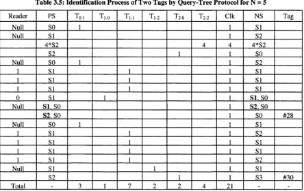
Table 3.5 shows tag identification process for this protocol for N = 5 with 2 tags present. The table is constructed by following Figure 2.3 (State diagram for Query-Tree Protocol) shown in section 2.3. In the 4th row of the table, under PS and NS columns, the states (S2) are multiplied by 4 and T2-2 and Clk have a value of 4 to show that the tag remains in state S2 for four clock cycles.
From the table, we can see at the 12th cycle upon receiving "0", Tag# 30 changes to SO while Tag# 28 jumps to SI (the bold font shows the state of Tag# 28). Tag# 30 then waits in SO until Tag# 28 is identified and then jumps to SI at the next rotation of identification process that starts at the 15' cycle.
Before deriving number of clock cycles (CLKQ) and the number of state transitions (TQ)
for the query-tree protocol under worst-case scenario for any N and n, first let us calculate CLKQ (n, 5)and TQ (n, 5) for N = 5 and different values of n.
*Q ~ "'0-1 + • ' l - O + •'1-2 + •'2-0
= rQ r( / i , J V ) - rw- r2.2 (3.7)
Where TQT(II, N) is the number of total state transitions including the self-loops ( T M and
T2-2) in Figure 2.3.
Table 3.5: Identification Process of Two Tags by Query-Tree Protocol for N = 5
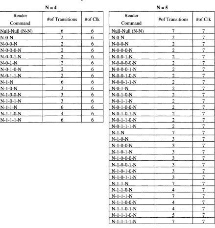
-Table 3.6: Commands used for Query-Tree Protocol with corresponding # of transitions and # of clock cycles for N = 4 and N = 5
N=4 N=5 Reader Command Null-Null fN-N) N-O-N N-O-O-N N-0-0-0-N N-0-0-1-N N-O-l-N N-0-1-0-N N-0-l-l-N N-l-N N-l-O-N N-1-0-0-N N-1-O-l-N N-l-l-N N-1-l-O-N N-1-l-l-N #of Transitions 6 2 2 2 2 2 2 2 6 3 3 3 6 4 6 #ofClk 6 6 6 6 6 6 6 6 6 6 6 6 6 6 6 Reader Command Null-Null (N-N) N-O-N N-O-O-N N-0-0-0-N N-0-0-1-N N-O-O-O-O-N N-0-0-0-1-N N-0-0-1-0-N N-0-0-1-1-N N-O-l-N N-0-1-0-N N-0-l-l-N N-0-1-0-0-N N-0-1-0-1-N N-0-1-1-0-N N-0-l-l-l-N N-l-N N-l-O-N N-1-0-0-N N-1-O-l-N N-1-0-0-0-N N-1-0-0-1-N N-1-0-1-0-N N-1-O-l-l-N N-l-l-N N-1-l-O-N N-1-l-l-N N-1-1-0-0-N N-1-l-O-l-N N-1-l-l-O-N N-1-l-l-l-N #of Transitions 7 2 2 2 2 2 2 2 2 2 2 2 2 2 2 2 7 3 3 3 3 3 3 3 7 4 7 4 4 5 7 #ofClk 7 7 7 7 7 7 7 7 7 7 7 7 7 7 7 7 7 7 7 7 7 7 7 7 7 7 7 7 7 7 7
For N = 5 and different number of tags (n), the worst case tag (Tag# 30) will follow the following pattern:
• For N = 5, n = 2:
We can see from Table 3.5, the commands from the reader are: N-N, N-1-1-1-0-N, and N-1-l-l-l-N; where N stands for Null.
From Table 3.6, we see that N-N command needs 7 numbers of transitions and 7 number of clock cycles. This is evident from Table 3.5, where the read cycle for N-N command ends after state jumps from S2 to SO, at the 7th cycle.
Hence in reference to Table 3.6,
C L K Q (2, 5) = 7 + 7 + 7 = 3*(5 + 2);
TQT (2, 5) = 7 + 5 + 7 = 2*(5 + 2) + 5;
• For N = 5, n = 3:
o The commands used are: N-N, N-1-1-0-N, N-1-l-l-N, N-1-1-1-0-N, N-1-l-l-l-N
Hence in reference to Table 3.6,
CLKQ (3, 5) = 7 + 7 + 7 + 7 + 7= 5*(5 + 2);
TQT (3, 5) = 7 + 4 + 7 + 5 + 7 = 3*(5 + 2) + (5 - 1) + 5;
• For N = 5, n = 4:
Hence in reference to Table 3.6,
C L K Q (4, 5) = 7 + 7 + 7 + 7 + 7 + 7 + 7 = 7*(5 + 2);
TQT (4, 5) = 7 + 4 + 7 + 4 + 4 + 5 + 7 = 3*(5 + 2) + 3*(5 - 1) + 5;
Using similar approach, for N = 5 and for the rest of the following tag distributions (n):
n = 5: CLKQ (5, 5) = 9*(5 + 2);
n = 6: CLKQ(6,5) = ll*(5 + 2)
n = 7: CLKQ (7, 5) = 13*(5 + 2) n = 8: C L K Q (8, 5) = 15*(5 + 2)
n = 9: CLKQ(9,5) = 17*(5 + 2)
TQT = 4*(5+2)+(5-2)+3*(5-l)+5; TQT = 4*(5+2)+3*(5-2)+3*(5-l)+5; TQT = 4*(5+2)+5*(5-2)+3*(5-l)+5; TQT = 4*(5+2)+7*(5-2)+3*(5-l)+5; TQT = 5*(5+2)+(5-3)+7*(5-2)+3*(5-l)+5; n = 10: CLKQ (10, 5) = 19*(5 + 2); TQT = 5*(5+2)+3*(5-3)+7*(5-2)+3*(5-l)+5;
After considering different Ns (N = 3, 4, and 6) for different ns, the following general equation is deduced:
F o r 2 < n < 2N _ 1,
Number of clock cycles, CLKQ:
Number of state transitions, TQT:
CLKQ={2n-l\N + 2) (3.8)
ifn = 2, TQT(2,N) = 2{N+2)+N
ifn = 3~4, TQT(3~4,N)=?(N+2)+[2{n-2)-llN-l)+N
TQT = TQT (n, N) = (l + 2)(N + 2) + [l(n - 2l)- \\N - 1 )
+ £[(2'-l)(tf-7 + l)]
7=1
= [2(n-2')-l](/V-/)+2('+ 1 )(/V-/ + 2 ) + ^ - t ^ (3.9)
Where 1 is given by (3.4).
For the self-loops, after performing similar analysis we obtained the following results:
ForN = 5:
n = 2: TM
n = 3: Ti.i
n = 4: Tw
n = 5: Ti.i
And
n = 2: T2-2 n = 3: T2-2 n = 4: T2.2 n = 5: T2-2
Therefore for any N and n, where 2 < n < 2" ',
ifn = 2, T1_l(2,N) = {N-2) + {N-l)
ifn = 3~4, 7;_,(3 ~ 4,A0 = [2(n-2')-l](iV-3)+2(yV-2)+(yV-l)
(5-2)+ (5-1)
(5-3) + 2*(5-2) + (5-l) 3*(5-3) + 2*(5-2) + (5-l)
(5-4) + 4*(5-3) + 2*(5-2) + (5-1)
ri_1= [ 2 ( n - 2 ' ) - l l 7 V - ( / + 2 ) ]+X { 2 ' -i^ - ( / + l - 7 ) ] }
;=o
= 2 n ( 7 V - / - 2 ) + 2( / + 2 )-2A/ + / + l (3.10)
ifn = 2, T2_2(2,N)={N-l)
ifn=3~4, T2_2(3~4,N)={N-l)+l
T2.2=(N-l)+±j = ( t f - l ) + / ( i ± T ) (3.11)
Therefore, the number of state transitions (TQ) will be:
TQ=TQT-Tx_x-T2_2=UAn (3.12)
For instance, for N = 5 and n = 8, we have C L K Q = 15*7 =105 and TQ = 2 + 4*8 = 34
3.3. Protocol-Level Analysis of Improved Query-Tree
Protocol
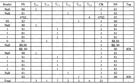
Table 3.5, used for query-tree protocol, can be modified for this protocol except that there will be a "Stop Send" (or an "SS") command from the reader at the start of the 4th cycle. Table 3.7 shows tag identification process for this protocol for N = 5 with 2 tags present. Even though the reduction of clock cycles is not evident through the comparison of Table 3.5 and Table 3.7, as the number of tags increases, the issuing of "SS" command further decreases the number of total clock cycles. For example for N = 5: if n = 4, C L K Q = 49
Table 3.7: Identification Process of Two Tags by Improved Query-Tree Protocol for N = 5 Reader Null Null SS Null 1 1 1 0 Null Null 1 1 1 1 Null Total PS SO SI 4*S2 S2 SO SI SI SI SI S1.S0 S2.S0 SO SI SI SI SI SI S2 -To-i 1 1 1 3 T1.0 1 1 T H 1 1 1 1 1 1 1 7 T,-2 1 1 2 T2-0 1 1 2 T2-2 4 4 Clk 1 1 4*S2 1 1 1 1 1 1 1 1 1 1 1 1 1 1 1 21 NS SI S2 S2 SO S2 SI SI SI S1.S0 S2.S0 SO SI SI SI SI SI S2 SO -Tag #28 #30
-Before deriving number of clock cycles (CLKIQ) and the number of state transitions (TIQ)
for the improved query-tree protocol under worst-case scenario for any N and n, let us observe the following points:
• Since improved query-tree protocol is similar to query-tree protocol with the exception of different performance in state S2; and since the numbers of transitions for both protocols do not include T2-2, the number of transitions for both cases stays the same.
Hence, the number of state transitions (TIQ) will be:
• Before deriving the number of clock cycles (CLKIQ), let us see the pattern of total
clock cycles for N = 5 and different number of tags (n):
o For n = 2, as shown in Table 3.7, the existence of "SS" after N-N command, won't alter the number of clock cycles and stays to be 7 (as compared to that the query-tree protocol. Hence,
• CLKIQ (2, 5) = 7 + 7 + 7 = 3*(5 + 2);
o For n = 3, the existence of "SS" after N-N command decreases the clock cycle in N-N read cycle from 7 to 6 (Table similar to Table 3.7 can be drawn to see the effect). Hence,
• CLKIQ (3, 5) = 6 + 7 + 7 + 7 + 7 = (5 + 1) + 4*(5 + 2);
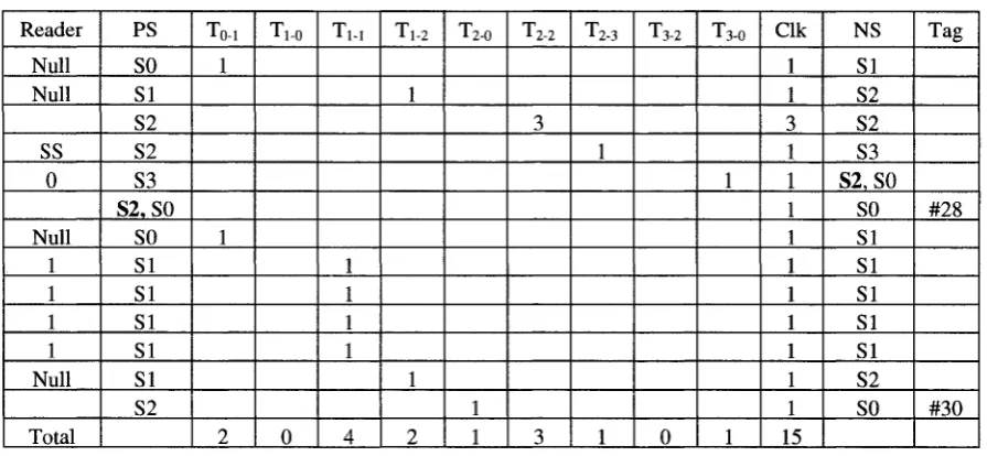
o For n = 4, as shown in Table 3.8, even if "SS" occurs after N-N, N-1-l-O-N, and N-1-l-l-N commands, it is only the existence of "SS" after N-N command that decreases the clock cycle in N-N read cycle from 7 to 6. Hence,
• CLKIQ (4, 5) = 6 + 7 + 7 + 7 + 7 + 7 + 7 = (5 + 1) + 6*(5 + 2);
o Similarly, for n = 8, "SS" occurs after N-N, N-l-O-N, N-1-0-0-N, N-l-l-N, N-1-l-O-N, and N-1-l-l-N commands. The existence of "SS" after N-N command decreases the clock cycle to 5; "SS" after N-l-O-N and N-l-l-N commands both decrease the clock cycle to 6. Hence,
Table 3.8: Identification Process of Four Tags by Improved Query-Tree Protocol for N = 5 Reader Null Null SS Null 1 1 0 Null SS Null 1 1 1 Null SS Null 1 1 0 0 Null Null 1 1 0 1 Null Null 1 1 1 0 Null Null 1 1 1 1 N PS SO SI S2 S2 SO SI SI SI SI. SO S2.S0 S2. SO SO SI SI SI SI S2 S2 SO SI SI SI. SO SI. SO SI SB. SO SO SI SI SI SI. SO SI. SO S2. SO
so
SI SI SI SI SI. SO S2. SOso
SI SI SI SI SI S2 To-i 1 1 1 1 1 1 1 TLO 1 1 1 1 4 TV, 1 1 1 1 1 1 1 1 1 1 1 1 1 1 1 1 Tl-2 1 1 1 T2-0 1 1 1 1 T2-2 3 1Clk NS SI S2 S2 SO SI SI SI SI. SO S2.S0 S2.S0 SO SI SI SI SI S2 S2 SO SI SI SI SI. SO SI. SO S2. SO
so
SI SI SIsi.
so
si.
so
After performing similar analysis, the following results were obtained for N = 5:
ifn = 2, CLKIQ(2,N)=3*{5+2)
ifn=3, CLKIQ(3,N) = {5+l)+4*{5+2)
ifn = 4, CLKIQ(4,N) = {5+l)+6*{5+2)
ifn=5, CLKIQ(5,N)=5+{5+l)+7*{5+2)
ifn=S, CLK,Q(8,N)=5+2*{5+l)+l2*{5+2)
ifn=16, CLtf/e(lf4A0 = (5-l)+2*5+4*(5+l)+24*(5+2)
Where, N=5
After considering different Ns (N = 3, 4, and 6) for different ns, the following general equation is deduced:
For any N:
F o r 2 < n < 2N - 1,
C L K i n^IQ = CLK101 + C L K IQl >JQ2
Where CLKIQ2 is the last term in the CLKIQ equation and CLKIQJ is the rest of the terms.
CLK102 and CLK101 are therefore,
n—3—k
CLK1Q2=3{N + 2)+2YJ{N + 2y ^(N + 2)
7=1 ;'=i
And
--{N + 2ll+n+k]
y
r n -2 -l)CLKIQ - CLKIQ1 + CLKIQ2
i-\
7=0
( (
int
V V
n — 2 O-+D_0
2 < J+ 2) +1 \(N + l-j)
[ " + [N + 2fl + n + k]
(3.16)
Where 1 is given by (3.4), and k by (3.17)
k = n — 3 (3.17)
As a special case, if n = 2m, then
m-\ |
CLKIQ(n = 2m)- 3(2(ra"1))(^ + 2)+ JT [(2""^ - \ \ N + 2-n)] n=l
Protocol-The Proposed Protocol
In this section we propose a new protocol that combines the binary-tree and query-tree protocols in order to reduce the number of state transitions and clock cycles under a worst-case scenario. Figure 4.1 shows the state diagram of the proposed protocol.
Same Start P r e f i x . ^ ^ / ;
( S I / State assignment Not s a m e — ^ \ S 0 : s t a n d bV
S1: Prefix Receiving Finished Finished S2: Sending Sending receiving S3: Mask receiving Interrupted^ I
. : > % Send remaining bits
Same'' ^ until interrupted
Figure 4.1: State diagram for the Combined-Binary-Query-Tree Protocol.
In this protocol, when a tag is in S2 and a collision is detected, it will go to another state, S3 (Mask receiving state), to receive a masking bit sent by the reader, instead of jumping to SO (as in case of the improved query-tree protocol). Table 4.1 shows tag identification process for the proposed protocol for N = 5 with 2 tags present and Table 4.2 for N = 5 with n = 4. In both tables, bold fonts used for states, indicate the status of the states in other tags while the worst-case tag (Tag# 30) is in state "SO".
As a result, the worst-case tag has to jump from SO to SI to S2 twice. In the proposed protocol, one of the tags will be identified by the masking bit (sent in S3), and the other by sending prefix bits only once. Thus, the worst-case tag will need less number of transitions and clock cycles for identification. For instance, for N = 5, n = 2, under the worst-case scenario, the improved query protocol uses 8 state transitions and 21 clock cycles; whereas this protocol uses 7 state transitions and 15 clock cycles.
Table 4.1: Identification Process of Two Tags by Combined Binary-Query-Tree Protocol for N = 5
Reader Null Null SS 0 Null 1 1 1 1 Null Total PS SO SI S2 S2 S3 S2.S0 SO SI SI SI SI SI S2 To-i 1 1 2 Ti-o 0 TV, 1 1 1 1 4 Tl-2 1 1 2 T2-0 1 1 T2-2 3 3 T2-3 1 1 T3-2 0 T3-0 1 1 Clk 15 NS SI S2 S2 S3 S2.S0 SO SI SI SI SI SI S2 SO Tag #28 #30
This protocol, however, needs an extra hardware in order to decrement its ID pointer while in S3. This is necessary because the tag receives a masking bit in S3 that needs to be compared with the previously sent bit.
By following the similar steps in deriving the number of clock cycles for the query-tree protocol, we can find the number of state transitions and number of clock cycles for the combined binary-query-tree protocol (again under worst-case scenario) as follows:
BQ — ^jV-*0-l "^M-0 +-M-2 "'"-'2-0 "'"-'2-3 "'"•'3-2 "'"-'3-0/
Where TBQT(II, N) is the number of total state transitions including the self-loops ( T M
and T2-2) in Figure 4.1.
Table 4.2: Identification Process of Four Tags by Combined Binary-Query-Tree Protocol for N = 5
Reader Null Null SS 0 SS 0 Null 1 1 0 1 Null Null 1 1 1 Null SS 0 Null 1 1 1 1 Null Total PS SO SI S2 S2 S3 S2. SO S3. SO S2. SO SO SI SI SI SI. SO SI. SO S2. SO SO SI SI SI SI S2 S3 S2.S0 SO SI SI SI SI SI S2 To-, 1 1 1 1 4 T,.0 1 1 T M 1 1 1 1 1 1 1 1 1 9 Tl-2 1 1 1 3 T2-0 1 1 T2-2 2 2 T2-3 1 1 2 T3-2 0 T3-0 1 1 2 Clk 31 NS SI S2 S2 S3 S2.S0 S3. SO S2. SO SO SI SI SI SI. SO SI. SO S2. SO SO SI SI SI SI S2 S3 S2.S0 SO SI SI SI SI SI S2 SO Tag #24 #26 #28 #30
• For N = 5, n = 2:
We can see from Table 4.1, the commands from the reader are: N-N-0 and N-1-l-l-l-N; where N stands for Null. Here the intermediate command "SS" is left out from N-N-0 command, but it is assumed to be within N-N-0 command. The same is true in the subsequent derivations.
From Table 4.1, we see that N-N-0 command needs 7 numbers of transitions and 8 number of clock cycles. This is evident from Table 4.1, where the read cycle for N-N-0 command ends after reading Tag# 28, at the 8th cycle. Hence,
CLKBQ (2, 5) = 8 + 7;
TBQT(2,5) = 7 + 7;
• ForN = 5, n = 3:
o The commands used are: N-N-0, N-1 -1 -N-0, and N-1 -1 -1 -1 -N. Hence,
CLKBQ (3, 5) = 8 + 8 + 7; TBQT (3, 5) = 6 + 7 + 7;
• For N = 5, n = 4:
o The commands used are (from Table 4.2): N-N-O-0, N-1-l-O-l-N, N-1-1-N-0, and N-1-l-l-l-N. Hence,
Using similar approach, for N = 5 and for the rest of the following tag distributions (n), the following pattern is developed:
Number of clock cycles:
n=2 n=3 n=8
CLKBQ = 2*(5+3)-l
CLKBQ = 2*(5+3)-l
CLKBQ = 2*(5+3)-l
Number of state transitions:
n=2 n=3 n=4 n=5 n=6 n=7 n=8 n=9
TB QT = 2 * ( 5 + 2 ) ;
TBQT = ( 5 + 1 ) + 2 * ( 5 + 2 ) ;
TBQT = (5-l) + (5+l) + 2*(5+2);
TBQT = (5-1) + 5 + (5+1) + 2*(5+2);
TBQT = (5-2) + (5-1) + 5 + (5+1) + 2*(5+2); TBQT = 2*(5-2) + (5-1) + 5 + (5+1) + 2*(5+2); TBQT = 3*(5-2) + (5-1) + 5 + (5+1) + 2*(5+2);
TBQT = 3*(5-2) + (5-1) + (5-1) + 5 + (5+1) + 2*(5+2);
n=10: TBQT = (5-3) + 3*(5-2) + (5-1) + (5-1) + 5 + (5+1) + 2*(5+2);
n=16: TBQT = (16-23-l)*(5-3) + 3*(5-2) + (5-1) + (5-1) + 5 + (5+1) + 2*(5+2);
For2<n<2 ,
CLK BQ=n{N + 3 ) - l (4.2)
And
7=1 7=1
= 2(M)+l(2-n)+Nn + 2 (4.3)
Where 1 is again given by (3.4).
For the self-loops, we have
ForN = 5:
n=2: n=3: n=4: n=5: n=6: n=8:
T M = ( 5 - 1 )
TM = (5-2) + (5-l)
T M = (5-3)+ (5-2)+ (5-1) TM = 2*(5-3) + (5-2) + (5-l)
TM = (5-4) + 2*(5-3) + (5-2) + (5-1) TM =3*(5-4) + 2*(5-3) + (5-2) + (5-1)
And n=2: n=3: n=4: n=5: n=8:
Therefore for any N and n, where 2 < n < 2 ,
ifn = 2, Tl_l(2,N) = {N-l)
ifn = 3~4, 7J_,(3 ~ 4,A0 = {n-3\N-3)+{N-2)+{N-l)
ri_1=(n-2'-l)[7V-(/ + 2 ) ] + X { 2 ' [ ^ - 7 - 2 ] } + ( ^ - l )
= n(N-l-2)+2{M)-N + l + l (4.4)
And
T2_2={N-l)-2 (4.5)
Therefore,
TBQ = TBQT - Tx_, - T2_2 =2{l + n) + 3 (4.6)
It should be mentioned that the states in Figure 4.1 can be encoded optimally as follows:
SO = 00, SI = 01, S2 = 11 and S3 = 10. While the Hamming distance between SO and S2
is 2, the number of transitions between them is only 1. Therefore, the power consumption
Four Tree Protocols
5.1. Protocol-level Comparison of the Binary, Query, and
Improved Query Tree Protocols
In this section, we evaluate the protocol level performance of the above three different protocols in terms of total number of state transitions, number of clock cycles, energy and power consumption, all under their worst cases. The number of state transitions is a key metric for estimation of power and energy consumption, while the number of clock cycles determines how fast the tags can be identified. Their ratio represents the transitions per clock cycle which measures energy consumption.
T -T
1 B,eq L B
T -T
1 Q,eq L Q
( CLKB ^ yCLK,Q j
f CLKQ A CLK
>QJ
T =T
1 IQ.eq 11Q
(5.1)
Thus, power consumption of the binary-tree, query-tree and improved query-tree protocols is proportional to, and measured by, TB, eq, TQ, eq and TIQ, eq, respectively.
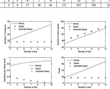
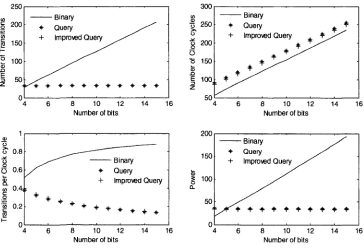
Comparison of the three protocols is shown in Figure 5.1 (for n = 4) and in Figure 5.2 (for n = 8) which is plotted using equations (3.5) ~ (3.8), (3.12) ~ (3.17), and (5.1). From both figures, it can be seen that the query-tree and improved query-tree protocols are preferable to binary-tree protocol in terms of number of transitions, and energy. Regarding power consumptions, by examining the two figures we can deduce that there is a region where the binary-tree is preferable over either of the two query-trees or vice versa. The point that divides the two regions is a function of N and n. For instance, for n = 4, Figure 5.1 shows that improved query protocol is better than binary-tree for any N. However, for n = 8, Figure 5.2 shows that the binary-tree will consume less power than the rest of the two protocols if N is less than 5.
In the region where n < nth, the improved query-tree has relatively lower power consumption than the query-tree, even though this is not evident from the two figures. For instance, for N = 5 if n = 8, TIQ, eq, = 34 and TQ; eq, = 35; and for N = 6 if n = 16, TIQ> «,, = 67 and TQ, eq, = 70.
Moreover the binary-tree uses lower clock cycles than the rest as shown by Figure 5.1 and Figure 5.2.
Table 5.1: Tabulation of nth for every N that determines the region n > nth where the binary-tree has
lower power consumption over the two query-tree types
N flu, 4 5 5 9 6 17 7 38 8 81 9 171 10 357 11 738 12 1515 80 60 40 20j 0 Binary + Query + Improved Query
6 7 8 Number of bits
10
100
S. 80
O 60
1
40s *20
rt.
+ Query
+ Improved Query *
d
* ^ - "
•
6 7 8 Number of bits
9 10
6 7 8 Number of bits
60 2 I 40 Q_ 20 n ri. + Query + Improved Query
'^^ * + + +
^ ^ ^
•
* i
6 7 8 Number of bits
9 10
Figure 5.1: Performance comparison of binary-tree, query-tree and improved-query-tree protocols
8 10 12 Number of bits
8 10 12
Number of bits
o 0.8 o 6 0.6
CD
g 0.4±
o
'I 0.2
2
K 0
p
* + + +
+
+ +
Binary Query Improved Query
+ + + +
8 10 12 Number of bits
14 16
150
1 100
0.
50
„. /
+ Query ^ ^
+ Improved Query s^
s ^
i: J^-f + + + + + + + + *.
n i . i i .
8 10 12 Number of bits
14 16
Figure 5.2: Performance comparison of binary-tree, query-tree and improved-query-tree protocols
5.2. Protocol-Level Comparison of the Proposed Protocol
with Binary and Improved Query Protocols
Equation (4.6) is modified to determine the equivalent value of the total state transitions for the proposed protocol (we still chose the improved query-tree protocol as a reference). The resulted equation is then,
T =T
1 BQ,eq l BQ
CLKBQ
CLKlQ j
(5.2)
0.8
0.6
IJ
0.2
6 7 8 Number of bits(N)
10 + + + + + + + - Binary Combined Improved Query '
+ + t + :
6 7 8 Number of bits(N)
10 100 60 40-' 20 • * • + + Binary Combined Improved Query + + + + + + ~
4 - ^ - ^ '
•
4-6 7 8 Number of bits(N)
6 7 8 Number of bits(N)
9 10
60
40
20
•#• Combined + Improved Query
^""^ + + +
" + + +
n i + + ^^^ . + '• + < 9 10
Figure 5.3: Performance comparison of binary-tree, improved query-tree and combined
of the Four Protocols at Different Levels of
Abstraction
Implementation of the Binary-Tree protocol, Query-Tree Protocol, Improved Query-Tree Protocol, and Combined-Binary-Tree Protocol, for a tag with N = 4, at different levels of abstraction namely, RTL level, Gate level and layout level is performed and the corresponding results are shown accordingly. For all protocols, the design was based on the worst-case scenario; that is Tag# 15 (1111) was selected for implementation. Hence, the following functional specifications are followed to design the logic:
The ID is represented by a 4 bit number, and Tag# 15 = 1111 is used for implementation; hence no memory is needed to store Tag# 15.
Inputs to the tag protocol circuit are •internal Reset
•signals coming from the reader: Start (or Null), Clock, Input_R (enquiring bit) •Output from the tag protocol circuit is Outl with the mapping showing in Table 6.1:
Table 6.1: Mapping of Outl and Out2 to the tag response
Response from the tag
No response
0
1
Outl
0
0
1
Out2
0
1
The output in our design (for Tag# 15) only uses Outl, because its ID = 1111, and it either responds a "No response" when it is in state "SO" or a bit from its ID (which is always "1"). Therefore, Out2 is not needed. But if a tag with an ID containing a "0" (for example Tag# 13 = 1101), we definitely need to have both Outl and Out2.
6.1. Implementation and Simulation of the Binary-Tree
Protocol
Figure 6.2: Schematic for Tag # 15 (N = 4): Binary-Tree Protocol
As can be seen from Figure 6.1, the operating frequency is 20MHz and it takes 1550ns for Tag# 15 to be read; hence the total number of clock cycles = 1550ns * 20MHz = 31. The reading starts at 75ns due to 'Reset' where the state is at SO. At 125ns, the state jumps to SI since Null (or Start) = 1. But at the next positive edge of the clock (at 175ns) the state returns to SO since the enquiry bit from reader = 0 and is different from the msb of the ID_byte which is 1, as a result, the tag signals a no-response situation by sending Outl = 0. Through successive enquiry-response pattern that resembles Table 1 (except for N = 4, n= 4) the reading continues and finally ends at 1625ns (where the tag is killed at S3).
The HDL code was synthesized using design_vision from Synopsys and the resulting schematic is shown in Figure 6.2.
Figure 6.3: Layout for Tag # 15 (N = 4): Binary-Tree Protocol
6.2. Implementation and Simulation of the Query-Tree
Protocol
After implementing Tag# 15 at different levels of abstraction using the Query-Tree Protocol, the corresponding results are shown in Figure 6.4, 6.5 and 6.6. The RTL Verilog code for this protocol was written based on Figure 2.3, but with the following additional information: the condition for transition from state "SO" to "SI" and from "SI" to "S2" is when "Null" = " 1 " and "Input_R" = "0". Appendix A.2.1 shows the full code.
From Figure 6.4, that shows the simulation result for the Verilog top-level module using SimVision, we can see that it takes 2100ns for Tag# 15 to be read. Hence, the total number of clock cycles = 2100ns * 20MHz = 42 clock cycles.
The waveform shown in Figure 6.4 is a result of a stimulus that follows a similar pattern outlined by Table 3.5, but with N = 4 and n = 4. The definitions of the variables used in the wave form are the same as the ones used in the Binary protocol case, except for the number of states. Here, the states are only SO, SI, and S2.
Figure 6.4: Simulation output for Tag# 15 (N = 4, n = 4): Query-Tree Protocol.
Figure 6.6: Layout for Tag# 15 (N = 4): Query-Tree Protocol
6.3. Implementation and Simulation of the Improved
Query-Tree protocol
Similarly, for Tag# 15 implementations at the different levels of abstraction using this protocol were performed and their corresponding results are displayed in Figure 6.7, 19 and 20. Similar to the RTL Verilog code of the Query Protocol, the RTL Verilog code for this protocol also assumes the condition for transition from state "SO" to "SI" and from "SI" to "S2" to be when "Null" = " 1 " and "Input_R" = "0". Appendix A.3.1 shows the full code.
synthesizing the Verilog code using design_vision and Figure 6.9 shows the final layout from Virtuoso.
From Figure 6.7, that show the simulation result for the Verilog code using SimVision, we can see that it takes 2100ns for Tag# 15 to be read, as a result, the total number of clock cycles = 2050ns * 20MHz = 41.
The waveform shown in Figure 6.7 is a result of a stimulus that follows a similar pattern as outlined by Table 3.7, but with N = 4 and n = 4. The definitions of the variables used in the wave form are the same as the ones used in the Binary protocol case, however like the Query protocol, the number of states are only SO, SI, and S2.
Baseline • ?5rts Cursor-Baseline = 2050ns
Figure 6.7: Simulation output for Tag# 15 (N = 4, n = 4): Improved-Query-Tree Protocol.