Mechanical and Laser Scribing For Use As Precision Shaping Techniques

(1)

ABSTRACT

LOVE, BRYAN MATTHEW. Mechanical and Laser Scribing For Use As Precision Shaping Techniques. (Under the direction of Jeffrey W. Eischen)

(2)

(3)

To my parents, Tom and Karen Love. Without your love and unending support,

(4)

Biography

(5)

Acknowledgements

I could not have completed this thesis without the help and guidance of many people. Many thanks to:

• Dr. Jeffrey Eischen, for guiding me through this project, offering tips and

suggestions when needed, and helping me catch my multitude of mistakes.

• Dr. Thomas Dow and the rest of the Precision Engineering Center, for

broadening my education and experience and making me consider things that are often overlooked.

• Dr. Ronald Scattergood, for the intuitive insights on the nature of mechanical

and laser scribing that led to some of the breakthroughs in my work.

• Donnie Moorefield and Hee Park of IBM, for practical information on laser

scribing and their assistance with the experimental work performed at IBM.

• and most of all, my friends and family, for supporting me, encouraging me,

(6)

List of Figures

1.1 Modern Hard Disk Drive. . . 1

2.1 Mechanical Scribing Process . . . 6

2.2 Line Dipole on Elastic Half-Space as a Model for Mechanical Scribing . . . 7

2.3 Definition of Finite Plate Mechanical Scribing Model. . . 8

2.4 Finite Element Mesh for Mechanical Scribing Simulations. . . . 10

2.5 Localized Stress Due to Mechanical Scribe . . . . 11

2.6 Mechanical Scribe Model Result for Full Scribe in x direction . . . . 12

2.7 Comparison of Scattergood Beam Theory Model with Finite Element Analysis . . . . 13

2.8 Deflections Generated by Partial Length Mechanical Scribes . . . . 14

2.9 Primary and Anticlastic Curvatures as a Function of Scribe Length . . . . . 15

2.10 Deflection Generated by Asymmetrical Scribe Placement . . . . 16

3.1 Laser Scribing Process. . . . 17

3.2 Illustration of Laser Scribed Slider . . . . 18

3.3 Laser Scribing Force Models . . . . 19

3.4 Row of Sliders . . . . 20

3.5 Slider Coordinate System and Curvatures Definitions . . . . 21

3.6 Interferometer Profile of Slider and Biquadratic Curve Fit . . . . 23

3.7 Experimental Results for Test Cases 1 through 6 . . . . 29

3.8 Experimental Results for Test Cases 7 through 12 . . . . 30

3.9 Experimental Results for Test Cases 13 through 16. . . . 31

4.1 Kelvin Coupling Boundary Conditions . . . . 36

4.2 Single Slider y-scribe Mesh . . . . 37

4.3 Mechanism for Creation of Residual Stress by Laser Scribing . . . . 40

4.4 Superposition of Dot Models Yielding End Force Model for Laser Scribes. . 40

4.5 Single Slider x-direction Scribe Model . . . . 41

4.6 Principal Stresses for Single Slider Model of a 1000 µm x-scribe . . . . 45

4.7 Finite Element Mesh for 747 µm x-direction Scribe. . . . 48

4.8 Finite Element Mesh for 1000 µm y-direction Scribe . . . . 49

4.9 Finite Element Mesh for 1005 µm x-direction Scribe . . . . 51

4.10 Comparison Between Shapes Produced by Scribing Single and Three Slider Models with an 800 µm y-scribe . . . . 55

5.1 Curvature versus Scribe Length for y-scribes . . . . 59

5.2 Curvature versus Scribe Length for x-scribes . . . . 60

5.3 Scaling Factor as a Function of Scribe Length. . . . 61

5.4 Asymmetrical Scribing Pattern . . . . 63

5.5 Curvature versus Scribe Length for Centered y-direction Laser Scribes . . . 67

5.6 Curvature versus Scribe Length for Centered x-direction Laser Scribes . . . 67

(9)

List of Tables

3.1 Interferometer Repeatability Test . . . 24

3.2 Laser Scribing Calibration Test Cases . . . 27

3.3 Experimental Laser Scribing Data . . . 31

4.1 Line Force System Calibration for y-scribing Models . . . 39

4.2 End Force System Calibration for y-scribing Models . . . 39

4.3 Results of FEA for x-scribes with Fm = 0.82 N . . . 42

4.4 Results of FEA for x-scribes with Fm = 0.925 N . . . 43

4.5 Mesh Specification for Scribes on Three Slider Models . . . 48

4.6 Three Slider Model y Calibration (Fm = 0.248 N) . . . 50

4.7 Three Slider Model x Calibration (Fm = 0.227 N) . . . 50

4.8 Three Slider Calibration for x-scribes with Revised x-1005 Model (Fm = 0.213 N) . . . 52

4.9 Three Slider Models for Test Cases 13 Through 16 (Fm = 0.213 N) . . . 53

5.1 Full Calibration for y-scribes (C = 0.04342) . . . 57

5.2 Full Calibration for x-scribes (C = 0.06027) . . . 58

5.3 Calibrated Results Using Scribe Length Dependent Scaling Factor . . . 62

5.4 Experimental and Predicted Results for Twist Test Pattern Using Original Calibration (Fm = 0.248 N) . . . 65

(10)

1 Introduction

1.1 Background and Objective of Research

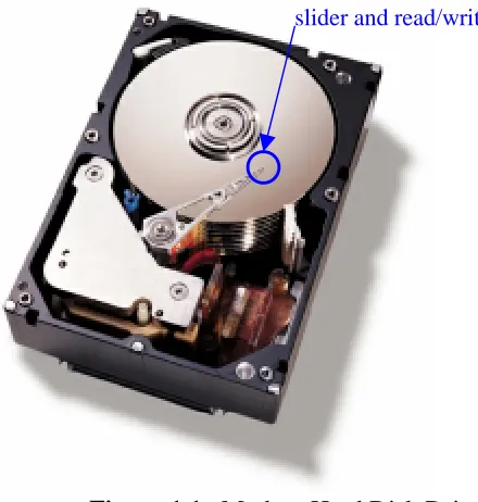
As the world becomes increasingly more dependent on computers, the speed and reliability of electronic storage (e.g. hard disk drives) has become a critical issue. Data density and hard drive speed are doubling approximately every eleven months. This rapid rate of increase demands constant refinement of materials processing and manufacturing techniques. A primary influence on the data density and speed of a hard drive is the flying height of the read/write electronics (head in the hard drive industry). The read/write heads are contained on a small ceramic slider that acts as an air bearing when the disk is in motion. Figure 1.1 shows a photograph of a typical hard disk drive.

As the storage disk rotates, it creates a boundary layer that causes the ceramic slider to “fly” over the surface. The shape of the slider determines how much lift or downforce is

(11)

generated and, therefore, the flying height of the read/write head. The slider flying height in modern hard drive is on the order of twenty-five nanometers and is decreasing rapidly due to industry demands (Tam, et. al. (1999)). Therefore, accurate control over the shape of the slider on the nanometer level is paramount to future performance and reliability improvements.

(12)

1.2 Modeling Techniques

(13)

1.3 Literature Review

There is little documentation of theoretical or experimental studies of scribing processes. Yoffe (1982) developed a twin-dipole model for indenting brittle materials— the technique utilizes a pair of experimentally calibrated dipoles on an elastic half space to model the stress field produced by indentation of a brittle material with a Vickers type indenter. Ahn, et. al. (1993) extended the indentation model to the scribing case by integrating Yoffe’s result. The integration produces the solution for a line dipole on an elastic half space—representing a mechanical scribe. Scattergood utilized Ahn’s solution to find the deflections produced by a mechanical scribe on a finite thickness plate by applying principles of superposition and a beam theory approximation. Further research at North Carolina State University conduced by Austin (2000), calibrated and verified Scattergood’s model using a particular ceramic material used in the construction of hard disk drive heads. The calibrated line dipole model (Scattergood-Austin) shows excellent correlation with experimental results. The previous research has shown that the line dipole model can successfully predict the deflections produced by mechanical scribing. The present research seeks to extend this model to scribing geometries and multiple scribe patterns not possible with the simplistic models used in the past.

(14)

(15)

2 Mechanical Scribing

2.1 Theoretical Model

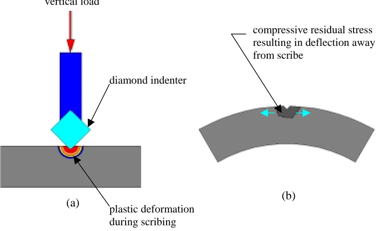
Mechanical scribing is the older (and more well documented) of the two scribing techniques. A mechanical scribe is produced by dragging the corner of a cubic indenter against the surface of a slider. This technique causes plastic deformation of the material and a localized area of compressive residual stress (see Figure 2.1a), along with a minute deflection of the slider away from the scribed side (see Figure 2.1b).

The determination of the residual stress field and predicting the deflections for the mechanical scribe is difficult; however, several models have been developed to predict deflections and stresses due to indentations and scribes. Yoffe (1982) used a pair of

Figure 2.1. Mechanical Scribing Process diamond indenter

vertical load

plastic deformation during scribing

compressive residual stress resulting in deflection away from scribe

(16)

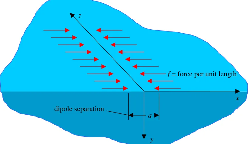
orthogonal force dipoles to model the residual stresses created by indentation on an elastic half-space. A previously developed model for mechanical scribing views the scribe as the superposition of a line of these dipoles (Ahn, et. al. (1993)). The forces in the scribing direction cancel during superposition (the end forces were neglected in Ahn’s model), resulting in the line dipole shown in Figure 2.2. This model has an exact

theoretical solution for both stress and deflection, but it requires that the associated structure be semi-infinite. Scattergood (2000) utilized this solution to develop a simple two-dimensional model designed to approximate the solution for a plate with finite dimensions (valid for the plane stress/strain case). The finite plate is cut out of the semi-infinite solid, and the reverse tractions are applied to the bottom and edge surfaces of the plate. Beam theory is then implemented to solve for the deflection created by the reverse tractions and the deflections are superposed with the deflections created by the line

y

f = force per unit length

dipole separation

a

x z

(17)

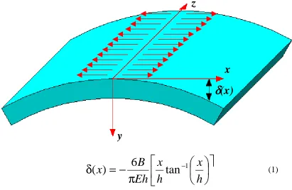
dipole. The result is an approximate solution for the finite plate with a line dipole. Figure 2.3 shows the resulting deflection and Scattergood’s solution.

Scattergood’s equation (equation 1) gives the deflection in terms of B (the dipole strength, B is the product of the force per unit length f and the dipole separation a), the thickness of the plate h, the elastic modulus E, and the position x. However, this equation cannot directly give the deflection. The model requires calibration since the magnitude of the line dipole is generally unknown. Austin (2000) approached this calibration directly by performing experiments with varying the vertical load on the scribing tool W (see Figure 2.1). Experiments were conducted using a material composed of alumina and titanium carbide (AlTiC). This material is currently used in read/write slider applications.

ù

ê

ë

é

÷

ø

ö

ç

è

æ

π

−

=

δ

−

h

x

h

x

Eh

B

x

)

6 tan

1

(

Figure 2.3. Deflection of Finite Plate Mechanical Scribing Model

x

y

z

δδδδ

(x)

(18)

Comparing the deflections generated by the model and the actual experiments, Austin developed a calibration equation that expresses B in terms of W for AlTiC:

2

291 .

0

516 .

0 0332

.

0 W

W

B

=

+

Using this empirically derived relation, Scattergood’s model can be used to predict the deflection of a mechanical scribe to within a few percent.

2.2 Finite Element Modeling for Mechanical Scribes

Several assumptions were made in the derivation of Scattergood’s theoretical solution. The actual elasticity solution to predict the deflection of a truly finite plate is unwieldy and impractical (and it possibly has no closed form solution), therefore numerical techniques are sought.

(19)

Mechanical scribing has a very localized effect—both Austin’s experiments and Scattergood’s model show that the scribe has very little influence on deflection beyond two to three scribe widths, and the stress fields shown by Yoffe (1982) and Ahn (1993) are also on this scale. Therefore, the finite element mesh must model this localized stress region—requiring a fine mesh around the scribe. However, after a small distance, the stress levels are negligible and the element size can be increased to speed up computational time without any impact on accuracy.

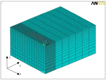
Considering the requirements for the scribing problem, a finite element mesh was developed in ANSYS 5.6 (a widely recognized and commercially available finite element package). The finite element mesh shown in Figure 2.4. utilizes quarter-symmetry

(symmetry planes on the faces on the left and right) to model a centrally located scribe.

Figure 2.4. Finite Element Mesh for Mechanical Scribing Simulations x

(20)

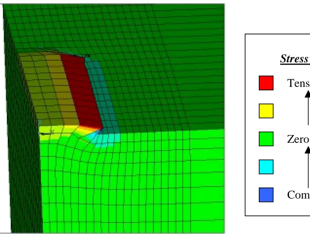
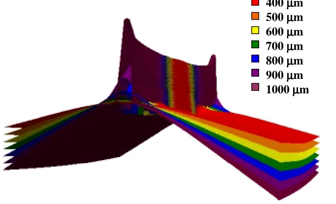
The quarter-symmetry slider model measures 0.625 mm by 0.5 mm by 0.3 mm, while the actual slider is 1.25 mm by 1.0 mm by 0.3 mm. To capture the stress field created by the line dipole scribe, a densely meshed region was created in the y direction around the scribe location. Figure 2.5 shows the stress field due to an applied scribe—note the localized effect of the scribe.

To model the scribe, a line force of magnitude 10.25 N/mm was applied all the way across the 0.5 mm direction (to mimic a complete scribe on a slider—an experiment previously performed by Austin and calibrated by Scattergood). The scribe separation was set at 8 elements (or 4 to the symmetry line), representing a dipole separation of 0.04167 mm. Using ANSYS 5.6, the solution was found for this model and is shown in Figure 2.6. Note that the large spike in the data is an artifact of the finite element model and should not be considered when comparing the finite element model to actual

Figure 2.5. Localized Stress Due to Mechanical Scribe

Compressive Zero Stress Tensile

(21)

deflections seen in experiments. One interesting aspect of the model is the small amount of curvature present in the direction parallel to the scribe. This curvature is often termed “anticlastic” curvature, and is an effect generated by Poisson’s ratio. The anticlastic curvature is small and in the opposite direction as the primary deflection. Assumptions made in Scattergood’s model do not allow the anticlastic curvature to arise in the solution.

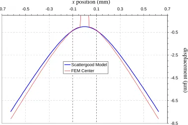
Further comparison between the finite element model and the beam theory model show that they agree within a few percent. Figure 2.7 shows a plot of the deflections predicted by the two models when B = 5 N/mm, E = 1 N/mm2, and h = 0.3 mm. Again, note that the spike in the center of the data in the finite element curve is an artifact of the analysis and would not be present in actual data. The tip deflections of the two models differ by 8.7%, and the general shape of the two data sets is similar. The difference in the tip deflection is due to Scattergood’s use of beam theory in his model—beam theory does not account for shear traction effects that are present in the finite element model.

(22)

Since the finite element analysis is inherently linear (as is the beam theory model), the calibration curve can simply be scaled and a similarly accurate calibration curve obtained. With an accurate calibration curve, the finite element technique can be used for varying scribe widths, as well as changing the orientation and placement.

2.3 Extension of Scribing Model Using Finite Elements

Mechanical scribing has been employed to control the shape of sliders for several years. However, to reach the levels of shape control necessary in the construction of a

-8.5 -6.5 -4.5 -2.5 -0.5

-0.7 -0.5 -0.3 -0.1 0.1 0.3 0.5 0.7

Scattergood Model FEM Center

Figure 2.7. Comparison of Scattergood Beam Theory Model with Finite Element Analysis

x position (mm)

dis

p

la

ce

me

nt

(

µ

m

(23)

new generation of sliders, better understanding of the deflections caused by mechanical scribes is needed. The Scattergood model (calibrated by Austin) allows accurate prediction of the deflection generated by mechanical scribes that extend across the full width of the slider. However, it does not allow scribes with a finite length or asymmetrically place scribes. It has been demonstrated that a calibrated finite element model can accurately model the scribing process. Also, the finite element model allows solutions for more complicated scribing geometries.

To determine the effect of scribe length, the finite element model was used to simulate mechanical scribes with varying lengths centered on the slider, oriented parallel

to the edges. The model varied scribe lengths from 200 µm to 1000 µm (full width

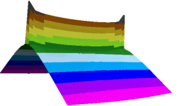
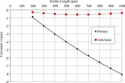
scribe). Figure 2.8 below shows the shape of the slider as a function of scribe length (200 and 300 µm scribes were eliminated from the plot for clarity). Note the anticlastic

curvature in each case. Figure 2.9 shows both the primary and anticlastic curvatures as a

Figure 2.8. Deflections Generated by Partial Length Mechanical Scribes

(24)

function of scribe length. Plotting trendlines (shown in Figure 2.9) through the data shows that both curvatures have a parabolic dependence on scribe length (R2 values are greater than 0.995). Using this parabolic dependence, the correct scribe length to obtain a desired deflection can be calculated—allowing precise control of the shape of the slider without intermediate measurement or closed loop control.

The use of finite elements also allows solution of other scribing geometries that would be very difficult through analytical techniques. Figure 2.10 shows the deflection generated by a scribe offset from the centerline of the slider. Scribing is frequently used as a curvature correction technique, and correcting for deflection not removed from the sliders by lapping could possibly require off-axis or even diagonal scribes. The finite element approach allows the deflection generated by these scribes to be predicted and,

-9 -8 -7 -6 -5 -4 -3 -2 -1 0

0 100 200 300 400 500 600 700 800 900 1000

Primary

Anticlastic

Figure 2.9. Primary and Anticlastic Curvatures as a Function of Scribe Length Scribe Length (µm)

(25)

through the use of superposition and a library of results, a scribing pattern to produce the desired deflection can be found.

In the past few years, new techniques have replaced mechanical scribing as a curvature adjustment technique. In production, mechanical scribing is time consuming and produces deflections on the order of 10 to 100 nm with reasonable precision. A new technique pioneered by IBM uses a laser to produce curvature on the sliders—it has the benefits of being much faster than mechanical scribing and produces deflections on the order of 1 nm with a high degree of precision. As with mechanical scribing, a model to predict the deflections produced by laser scribing is needed as the demands on data density and hard drive speed increase.

anticlastic

(26)

3 Laser Scribing

3.1 Background and Theoretical Approach

Laser scribing is a newer technique for controlling the shape of sliders. IBM, one of the major manufacturers of read/write heads in the United States, pioneered this field and created a system known as the Laser Curvature Adjust Technique (LCAT) (Tam (1999)). Figure 3.1 illustrates the simple technique: a pulsed laser is focused on the surface of the ceramic slider, and with sufficient power input a small circle of material is melted. The solidification of this material results in a localized stress around the circle— the ceramic shrinks as it solidifies and the material outside the dot is placed in tension. If a line of dots is created, the spacing between the dots can be decreased until it resembles a solid line. Studies at IBM have shown that as the dot spacing is decreased, the resulting deflection saturates, producing a continuous, repeatable “scribe” (Tam, et. al. (1999)). The laser can be accurately controlled by a set of galvo mirrors, thus allowing the LCAT

Figure 3.1. Laser Scribing Process pulsed laser

residual tensile stress.

(27)

system to place scribes of varying lengths anywhere on the surface of the slider.

The stresses and deflections created by laser scribing differ from mechanical scribing in several ways. The most obvious is that laser scribes produce residual tension, rather than the compression, resulting in the slider bending towards the scribe as show in Figure 3.1. Secondly, laser scribes produce appreciable curvature in the both directions relative to the scribe axis. These curvatures are of the same order of magnitude and in the same direction (shown in Figure 3.2). Compare this response with the very small, opposite-direction anticlastic curvature generated by mechanical scribing.

While the two types of scribing generate different deflections, they both induce localized areas of stress. The line dipole force system that accurately modeled mechanical scribing can be extended to the laser scribing case with some modification. The direction of the forces needs to be changed; the curvature generated by laser scribing is in the reverse of the curvature generated by mechanical scribing. The line dipole, however, does not produce the curvature in the parallel direction as seen in laser scribing.

(28)

An extension to the model must be made to compensate for this effect. Figure 3.3 shows two proposals for force systems to model laser scribing. In both models, the familiar line dipole forces fM (force per unit length) produce curvature perpendicular to the scribe. The parallel curvature is generated by the application of a uniform force fm (force per unit length) in the line force model, while the end force model relies on forces Fm to produce the parallel curvature. Just as with the mechanical scribing, these models must be calibrated with experimental results.

3.2 Nomenclature

The read/write head industry has developed its own terminology to describe the size and shape of sliders. The particular terms and conventions presented here are those used by IBM. The sliders are constructed of an alumina-titanium carbide (AlTiC) ceramic, and are approximately 1.25 mm by 1.07 mm by 0.30 mm (this size is know as the “pico” slider). Forty-four sliders are attached along the 1.25mm edge, resulting in a 47mm by 1.25mm by 0.3mm row (shown in Figure 3.4). The two large surfaces are known as the air bearing surface (ABS side) and the flex side. The ABS side flies over the surface of

Figure 3.3. Laser Scribing Force Models

fM fM

fm Fm

(29)

Crown = -C4L2/4

Camber = -C3W2/4

Twist = -C5LW

the storage disk, while all scribing is performed on the flex side. The shape of the ABS side determines the flying height, so each slider’s ABS side is measured while the flex side is scribed. The out of plane deflection w, of the ABS side is fitted with a biquadratic curve as follows:

w = f(x,y) = C

0

+ C

1

x + C

2

y + C

3

x

2

+ C

4

y

2

+ C

5

xy

where x and y and z are defined in Figure 3.4. The first three coefficients describe the best-fit plane through the surface (thus removing any rigid body rotations from the data). The final three coefficients define curvatures that are important in the aerodynamics that determine the flying height. These curvatures are normalized and defined as crown, camber, and twist:

where L and W are the length and width of the ABS side (L = W = 1mm for IBM’s purposes). The negative signs define positive curvature as curvature that lift the corners away from the storage disk. Figure 3.5 shows a graphical representation of crown, camber, twist, and the coordinate system. Note that in this diagram, crown is positive and camber is negative.

47 mm 1.25 mm

x y z

Figure 3.4. Row of Sliders

thickness = 0.3 mm

(2)

(30)

Crown is the primary influence on slider flying height, but control over camber and twist is essential for performance improvement. Currently, crown can be controlled accurately with the LCAT system—usually, to the nearest nanometer. Due to current capabilities and demands, the amount of camber created by the scribing pattern is directly proportional to the amount of crown and there is very little compensation for twist. The asymmetry represented by twist is a major problem in slider construction; in fact, one of the major objectives of this project is to develop scribing patterns to remove twist from a slider.

Crown

Twist

Camber

X Y Z

Leading Edge

Trailing Edge

ABS Side

Flex Side

Crown

Side View of Slider Along X axis ABS pad

Figure 3.5. Slider Coordinate System and Curvature Definitions

(31)

3.3 Experimental Metrology

Measuring and handling of parts on this scale can be challenging and requires special considerations. To provide an accurate representation of industrial techniques and practices, all tests were conducted at IBM-San Jose, utilizing their laser scribing (LCAT) and metrology equipment. As stated previously, sliders are measured and scribed while still part of a row—making handling much simpler and requiring less complicated fixtures and shorter set up times. Currently, sliders are scribed and measured in a closed-loop system, described in more detail by Tam (Tam, et. al. (1999)). The LCAT accepts fixtures that hold 24 rows (a total of 1056 sliders) utilizing a vacuum system. An x-y positioning stage permits any slider to be viewed (from both sides) and scribed on the flex side. Once the sliders are loaded in the LCAT, each is scribed several times and curvatures are measured using an internal optical measuring device. The process is repeated until the sliders reach a desired shape. The effect of a single scribe is not directly observed in the process; the final shape of the ABS side is the only consideration. Therefore, to accurately study the effects of scribes, a different technique is needed.

(32)

then scribed, and the row was measured again. Subtracting the two slider profiles (before and after) gives the distortion generated by the scribes.

There are several issues that affect the accuracy and repeatability of this technique. Ideally, the actual measured profile would be used to describe the shape of the slider. However, the material properties of the AlTiC prevent a repeatable profile—the alumina and titanium carbide grains have different optical properties, resulting in a profile that has a very large deviations that are not physically present (as shown in Figure 3.6). Subtracting the before and after profiles can result in amplifying these deviations,

which can hide the actual shape of the slider. So, the biquadratic parameters (crown, camber, and twist) are used to describe the shape of the slider. The three parameters provide the average curvature in each direction, essentially acting as a low pass filter on the data. As mentioned previously, the biquadratic curve fit removes any rigid body rotation from the data, so the curvatures found before and after scribing and can be subtracted to directly give the curvature created by the scribing pattern.

(33)

Due to the high degree of precision necessary in the measurement of the sliders, the repeatability of the measurements must be considered when collecting data. To test the interferometer, curvatures from six sliders were recorded and the sliders were removed from the interferometer. Some time later the sliders were measured again without any modifications. Table 3.1 shows the results of this test. The average repeatability of a single measurement is 0.098 nm. However, recall that to determine the

effects of a single scribe, measurements are required before and after a scribe. With the data scattered positive and negative, the actual determination of a scribe’s effect could

vary approximately ±0.2 nm. This variation is significant in determining what scribing patterns are admissible, and how many measurements are needed to have an accurate representation of the curvatures created by a scribing pattern.

3.4 Scribing Patterns

The scribing patterns used to calibrate the laser scribing model needed to encompass the LCAT’s range of capabilities in scribe length, scribe location, and scribe direction. To remove any variation in scribe strength, the laser parameters (power,

Table 3.1. Interferometer Repeatability Test

Row No. Slider No. Crown Change

(nm)

Camber Change (nm)

Twist Change (nm)

1 10 -0.08 -0.03 0.18

1 20 0.12 -0.09 -0.09

3 10 -0.11 0.16 -0.12

3 20 0.07 -0.04 0.06

4 10 0.06 0.11 -0.17

(34)

frequency, and beam width) were held constant—IBM has experimented extensively with these parameters and determined an optimal setting. There are a few limitations on scribe placement and length. The scribes cannot cross—interaction effects create problems with

the surface of the slider. The scribes are approximately 40 µm wide; placing an ultimate limit on scribe spacing. Also, the scribes cannot be placed too close to the edges of the slider—one edge contains the read/write electronics which are distorted by the residual stress induced by the laser scribes. To prevent creating additional twist, scribes are usually made in the x and y directions and are symmetric with respect to the other axis.

Ideally, several single scribes of varying locations and lengths would be used to calibrate the model. Experimental history at IBM shows that a single scribe creates approximately 0.6 nm of curvature in the crown direction. This level of curvature is very small considering that the repeatability of a single measurement is roughly 0.1 nm; the experiments could easily see 16% (or more) error just due to measurement repeatability. This error can be reduced by repeating the scribe pattern and averaging the results; using single scribes for calibration purposes, however, requires an impractical number of measurements. To reduce the number of required measurements, the overall deflection (and thus the number of scribes) needs to be sufficient to reduce the error. Three scribes is the minimum number of scribes to reduce the measurement error less than 10% for a single measurements; ten measurements reduces the average error to 2.5%.

(35)

and a pattern that contains all of the scribes present in the other two. If the curvatures of the “superposed” pattern are the sum of the curvatures of the two independent patterns, then superposition is obeyed. This exact test was performed and the results confirmed that laser scribing obeys superposition for non-overlapping scribes (see Experimental Results). Since the scribes obey superposition, individual scribes can be modeled and their curvatures added to give the curvature generated by a certain scribing pattern—a versatile technique that allows a library of single-scribe solutions to represent a multitude of scribing patterns.

The set of experiments used for calibration purposes must give an accurate indication of the range of capability of the LCAT system and must be simple enough to model accurately. To accomplish this, all scribes were made in the x and y directions and were centered on the slider. Therefore, all of the calibration scribing patterns are symmetric with respect to the x and y axes, thus theoretically eliminating any twist generation. Calibration of symmetric patterns is straightforward—forces fM and FM (or fm, refer to Figure 3.2) are varied until the desired crown and camber are reached.

To encompass the range of ability of the LCAT system, the patterns must show variation in scribe length and placement. For scribes in the y direction, the length can

vary from approximately 600 µm to 1000 µm; any shorter and the deflections become

smaller than can accurately be measured (for three 600 µm scribes, the crown is 1.6nm),

any longer and the scribe interferes with the read/write head. For x-direction scribes, the

range of scribing lengths is from approximately 350 µm to 1005 µm. Scribes can be placed at nearly any location on the slider and therefore, the minimum spacing is

(36)

scribes has a limit—the 120 µm at each end of the slider (in the y direction) is removed

from the data set to prevent the roll-off from affecting the curvature parameters. Using this set of parameters, a calibration set was created with sixteen experiments. Table 3.2 describes the geometry of all sixteen laser scribing patterns. Note that test cases 6, 7, and 8 constitute a superposition test. This set of test cases encompasses a wide range of the LCAT’s capabilities and provides adequate information to calibrate the model.

Table 3.2. Laser Scribing Calibration Test Cases

Test Case Direction No. of Scribes Length (µm) Spacing (µm)

1 y 3 1000 80

2 y 3 800 80

3 y 3 600 80

4 y 3 1000 40

5 y 3 1000 240

6 y 3 800 160

7 y 4 800 160

8 y 7 800 80

9 x 3 1005 80

10 x 3 747 80

11 x 3 556 80

12 x 3 365 80

13 x 3 1005 400

14 x 3 1005 200

15 x 3 1005 40

(37)

3.5 Experimental Scribing Results

The sixteen test patterns were produced and measured using the following method: 1. ABS sides of 44 sliders (1 row) measured and recorded using the

interferometer.

2. Sliders loaded into LCAT, scribing patterns programmed and scribed with pauses between each slider (to prevent thermal effects).

3. Sliders removed from LCAT; flex sides examined under optical microscope to verify scribe placement and lengths.

4. ABS sides of sliders measured and recorded using the interferometer.

(38)

Test Case 1

3 y scribes L = 1000 µm Spacing = 80 µm Crown: 1.65 nm Camber: 2.65 nm Twist: -0.05 nm

Test Case 2

3 y scribes L = 800 µm Spacing = 80 µm Crown: 1.82 nm Camber: 2.55 nm Twist: 0.09 nm

Test Case 3

3 y scribes L = 600 µm Spacing = 80µm Crown: 1.66 nm Camber: 1.96 nm Twist: 0.21 nm

Test Case 4

3 y scribes L = 1000 µm Spacing = 40 µm Crown: 1.58 nm Camber: 2.54 nm Twist: 0.02 nm

Test Case 5

3 y scribes L = 1000 µm Spacing = 240 µm

Crown: 1.56 nm Camber: 1.83 nm Twist: -0.03 nm

Test Case 6

Crown: 1.91 nm Camber: 2.35 nm Twist: 0.06 nm

(39)

Test Case 7

Test Case 8

7 y scribes L = 800 µm Spacing = 80 µm Crown: 4.64 nm Camber: 5.37 nm Twist: -0.53 nm

Test Case 9

3 x scribes L = 1005 µm Spacing = 80 µm Crown: 3.69 nm Camber: 1.59 nm Twist: -0.27 nm

Test Case 10

3 x scribes L = 747 µm Spacing = 80 µm Crown: 2.59 nm Camber: 1.59 nm Twist: 0.18 nm

Test Case 11

Test Case 12

(40)

Test Case 13

3 x scribes L = 1005 µm Spacing = 400 µm

Crown: 1.75 nm Camber: 21.72 nm

Twist: 0.07 nm

Test Case 14

Test Case 15

Test Case 16

(41)

Examination of the data reveals some interesting conclusions (both about metrology and the scribing results). The standard deviations are on the order of 0.10 nm —very close to the uncertainty predicted by the repeatability experiment, meaning that the laser scribes themselves are consistent and repeatable within the measurement error. The presence of small amounts of twist in the data indicates that the scribes may not have been completely symmetric with respect to the x and y axes or the scribing geometry is not as simple as once thought. The raw data (given in Appendix B) indicates that the test cases showing the most twist were performed on rows that were highly twisted before scribing—the twist could possibly be generated because the scribes are placed on an asymmetrically curved surface. Furthermore, the average value of twist and the standard deviations for all three curvatures can be reduced by removing the sliders from the end of the rows from the data set. For example, if the first slider from Test Case 10 is removed,

Table 3.3. Experimental Laser Scribing Data

*Note: See Table 3.2 for scribing geometries

Test Case No. Samples Crown (nm) Camber (nm) Twist (nm) Crown (nm) Camber (nm) Twist (nm) 1 8 1.6464 2.6527 -0.0500 0.1726 0.1764 0.1998 2 10 1.8230 2.5480 0.0910 0.1739 0.0991 0.0700 3 11 1.6573 1.9600 -0.2127 0.1106 0.0822 0.1761 4 11 1.5800 2.5373 0.0155 0.1254 0.0940 0.2267 5 11 1.5573 1.8273 -0.0345 0.0855 0.0413 0.1882 6 7 1.9114 2.3457 0.0571 0.0871 0.0640 0.1751 7 7 2.8414 2.9443 -0.1514 2.5020 0.1336 0.3235 8 7 4.6371 5.3686 -0.5314 0.3661 0.2746 0.3321 9 11 3.6873 1.5909 -0.2700 0.2050 0.1015 0.3814 10 11 2.5873 1.5855 0.1764 0.2098 0.0805 0.2948 11 11 1.8209 1.2418 -0.0127 0.1487 0.0540 0.1851 12 11 1.1082 0.8373 -0.1091 0.0672 0.0307 0.1283 13 44 1.7470 1.7218 0.0661 0.2977 0.1417 0.3841 14 11 3.0745 1.6900 -0.0318 0.2934 0.0621 0.4065 15 11 3.6573 1.5609 -0.5109 0.2096 0.1188 0.4393 16 11 4.1709 3.2345 -0.4400 0.3622 0.2631 0.3887

(42)

(43)

4 Finite Element Modeling

4.1 Background

A robust model of any scribing system must be capable of accurately modeling any scribing geometry. Analytical models can produce accurate results for mechanical scribes in simple geometric patterns (see Sections 2.1 and 2.2). Applying this type of analytical solution to mechanical scribes with finite lengths is impractical. Furthermore, all proposed laser scribing models (see Section 3.1) require finite length scribes and generate end effects. So, a flexible and accurate numerical technique was sought that allows three-dimensional solutions of any scribing geometry.

Finite element analysis offers geometric flexibility and high accuracy with proper considerations. For the scribing models, a basic linear elastic finite element analysis was chosen because three dimensional elasticity has previously been used to accurately model residual stresses (Ahn (1993)) and it allows fast and accurate solutions. The technique relies on elements that represent differential units, assembled into a mesh that represents the overall geometry. A large system of equations represents an approximation to the actual elasticity solution. The solution converges as the number of elements increases.

(44)

stress, the accuracy of the model can be improved. Scribing creates a very localized stress field (as shown in Figure 2.5) that requires a very high mesh density near the scribe. However, the stress is negligibly small a short distance from the scribe, and the mesh density can be rather coarse without affecting accuracy. Also, careful use of symmetry allows a reduction in the number of elements used by a factor of two without adding any additional elements or affecting computational time. Taking these facts into consideration, the desired accuracy can be achieved with the minimum required computational time.

(45)

Mechanical scribing has been extensively discussed in Chapter 2, with the finite element modeling addressed in Sections 2.2 and 2.3. However, the bulk of the finite element work was conducted on laser scribing. The following work discusses the development of the laser scribing model and its calibration.

4.2 Laser Scribe Force Model Specification

The experimental results in Section 3.5 show that laser scribes generate curvature parallel and perpendicular to the scribe. Qualitatively, both the line force and the end force models (discussed in Section 3.1) produce deflections similar to those seen in the experimental results. To determine which model best fits the experimental data, a single slider finite element model was created to model scribes along the y direction. The model employs symmetry across the y-axis to conserve elements, and uses the Kelvin coupling placed on the corners of the slider for boundary conditions. Scribing patterns matching

Figure 4.1. Kelvin Coupling Boundary Conditions x

y z

2

1

(46)

those performed experimentally were modeled using both the line force and the end force systems.

The single slider model uses the techniques discussed in Section 4.1. The scribe region is 0.25 mm wide, with 24 elements spanning its width. Four elements are placed

between the line forces, giving a dipole separation of 50 µm. There are 20 elements

across its width, allowing scribes of 600, 800 and 1000 µm (three scribe lengths used in

the experiments) to be modeled easily. Figure 4.2 shows the finite element model with

the 1000 µm scribe. Note the coarse mesh outside of the scribe region—reducing the size

of the model without impacting the accuracy of the solution. The scribing region can be

Figure 4.2. Single Slider y-Scribe Mesh

x

(47)

moved from three single-scribe models can be superposed to give the solution for a single three-scribe model (simulating one of the experiments).

To compare the finite element solutions to the experimental results, the ABS side of each model is fitted with a biquadratic and the crown, camber, and twist are computed (in this case, twist is geometrically eliminated). The curvatures can be added for the three models representing the experimental scribes giving a total crown and camber for the model. The finite element model has not been calibrated—so the solution will not exactly match experimental results. However, the model is linear, so if the crown to camber ratio is correct, it is a simple matter of using a linear scaling factor to obtain the correct deflections.

The end force and the line force systems were applied to the finite element model

using the following guidelines. The line dipoles were applied with 50 µm spacing, with a magnitude of fM = 20 N/mm. The magnitudes of the line forces (fm) and the end forces (Fm) were varied until the crown to camber ratio of a specific model matched that of the experimental results to a reasonable degree of precision. The modulus of elasticity was taken to be E =1 N/mm2(the results, however, can be scaled linearly) and Poisson’s ratio was taken to be 0.2. The model used for calibration is Test Case 1, consisting of three

1000 µm, y-direction scribes with a spacing of 80 µm. The experimental results gave a

crown of 1.65 nm and 2.65 nm of camber, for a crown to camber ratio of 0.623. Varying the fm in the line force model, gave a crown to camber ratio of 0.616 for Test Case 1 (a 1.11% error) with fm = 1.50 N/mm. Using this line force as the calibration, Test Cases 2 through 8 were computed using similar models. The results are shown in Table 4.1. The

(48)

error increases as the scribe length is decreased. It is interesting to note that the error is relatively consistent for any given scribe length—an important indication that the line dipole model (that generates camber in this case) produces accurate results but the line forces do not accurately represent the stresses generated parallel to the scribe.

Performing a similar calibration for the end force model gives a crown to camber ratio of 0.615 for Test Case 1 (1.32% error) for an end force of Fm = 0.82 N. Performing the rest of the analyses for Test Cases 2 through 8 gave the results shown in Table 4.2. The results show that the end force model is quite accurate for modeling the y-direction

Finite Element Model Experimental

Test Case Crown Camber Ratio Ratio % error

1 130.96 213.03 0.615 0.623 1.32

2 124.42 164.59 0.756 0.714 5.87

3 108.17 128.19 0.844 0.847 0.37

4 130.92 218.66 0.599 0.622 3.74

5 131.58 157.88 0.833 0.852 2.18

6 124.48 147.66 0.843 0.813 3.69

7 166.01 172.63 0.962 0.966 0.45

8 290.49 320.29 0.907 0.864 4.97

Table 4.2. End Force System Calibration for y-scribing Models

1 136.01 220.92 0.616 0.623 1.18

2 84.43 173.26 0.487 0.714 31.75

3 50.16 136.54 0.367 0.847 56.63

4 135.95 226.73 0.600 0.622 3.60

5 137.01 164.08 0.835 0.852 1.99

6 84.37 156.04 0.541 0.813 33.49

7 112.38 183.42 0.613 0.966 36.57

8 196.75 339.46 0.580 0.864 32.92

(49)

scribes—over all eight of the test cases, the maximum error is less than six percent. Further insight into the validity of the end force model can be obtained by examining the process by which the residual stress is created within the material. The laser scribe is actually a collection of overlapping “dots” that are created by melting the surface material with a pulsed laser. Figure 4.3 illustrates this process. A single dot of

material is melted by a laser pulse, and the solidification (and the resulting contraction) of the melted material produces a strain on the bulk of the slider. The resulting residual stress is tensile in the region immediately surrounding the scribe. A simple force model

(shown in Figure 4.3) can be used to model the residual stresses produced by the Melted AlTiC

Strain created by solidification of AlTiC

Force model for stress produced by a single dot

Figure 4.3. Mechanism and Model for Creation of Residual Stress by Laser Scribing

dot spacing

(50)

are placed closer and closer together, the stress fields produced by each individual dot begin to overlap. The tensile forces begin to cancel one another, as illustrated in Figure 4.4. Eventually, the dot spacing is reduced to the point where the dots begin to overlap and the stress along the scribe is completely cancelled, except for the stress produced by the last dot on each end, resulting in a force system resembling the end force system.

4.3 Single Slider Models

The initial attempt to model the scribing process focused on finite element models of single sliders. The finite element meshes modeled a slider measuring 1.25 mm by 1.0 mm by 0.3 mm, employing a symmetry plane to reduce the number of elements. The scribes, as with the test cases, were limited to the x and y directions, so two adaptable meshes were developed—one for x-direction scribes (shown in Figure 4.5) and the other for y scribes (shown in Figure 4.2).

Figure 4.5. Single Slider x-direction Scribe Model

x

y

(51)

The two finite element meshes utilize the same techniques that were discussed in Section 4.1 for providing accurate solutions with minimal computation time. Both meshes employ symmetry planes on the centerline (the x-axis for the y scribe model and the y-axis for the x scribe model) to reduce the number of elements without impacting the accuracy of the solution. Also, the scribing region of both meshes is 0.25 mm wide, is divided up into 24 elements along its width, and the dipole separation is set at 4 elements

(or 50 µm). Through the use of input file structures, the scribing region can be translated to give the scribe a different placement without drastically altering the mesh. These two meshes, with minor modifications, were used to model all 16 test cases.

The end force system was chosen to model the scribes, based on the sample calibrations (shown in Section 4.2) which yielded very accurate results for the y-scribe models. The calibration used to generate the data in Table 4.2 (Fm = 0.82 N) was used to model the x-scribes. The results for test cases 9 through 12 are shown in Table 4.3. The

errors are much higher than in the y-scribe case, however, the results are closely grouped together. If the x-scribe models are calibrated as an independent set, the errors can be significantly reduced. A re-calibration with test cases 9 through 12 yielded an end force of Fm = 0.925 N. The data is shown in Table 4.4. The maximum error is now approximately 5%, a reasonably acceptable value.

9 247.84 95.01 2.608 2.311 12.86

10 197.16 97.80 2.016 1.708 18.04

11 146.32 87.96 1.663 1.444 15.18

12 95.59 63.82 1.498 1.262 18.70

(52)

The need for separate calibrations depending on scribe direction raises some interesting issues. Theoretically, if the model perfectly matched the experimental conditions, a single force system (with a single calibration) would be able to model any scribing geometry. However, in the development of this model, many assumptions were made to make the modeling simple and flexible. The most obvious assumption relies on the force model itself—the actual mechanism for distortion is a melt/solidification process that produces residual stress. The force model provides a simple and possibly accurate approximation to the residual stress, but it does not work from first principles and therefore, can be a source of inaccuracy or approximation. Another assumption is that the AlTiC material is elastic and isotropic. One possible explanation for the inconsistency in results between the two directions is that the processing of the material gives it different properties in the x and y directions—the sliders are come from a 125mm diameter (1.2 mm thick) wafer that is sectioned and lapped to form the rows. Also, there

is the thin layer of electronics covered by a thin (50 µm) layer of alumina on one edge— however, the material properties of alumina are very close to that of AlTiC, so very little error would be expected

The geometry of the heads themselves leads to several more assumptions. All of the finite element models are exactly 1.25 mm by 1.0 mm by 0.3 mm, but while the

9 243.37 111.08 2.191 2.311 -5.20

10 193.89 113.40 1.710 1.708 0.10

11 144.04 101.50 1.419 1.444 -1.74

12 94.22 73.46 1.283 1.262 1.64

(53)

actual rows and sliders do very slightly (+/- 1%). Also, the models assume that the slider is initially flat, but experimental metrology shows that the heads have a peak to valley deviation of 5 to 10 nm before scribing—the amount of deflection comparable to 3 or 4 scribes. The most obvious geometric assumption is modeling a single slider—as stated previously, all the sliders were scribed and measured as part of a 44-slider row (see Figure 3.3). This assumption produces incorrect boundary conditions on two edges of the slider, something that could effect certain scribing arrangements more than others, possibly producing considerable error.

(54)

specific to the individual sliders that were experimented with. However, all sliders are scribed as a part of a row—and the difference in boundary conditions between a single slider and a slider as a part of a row could make a significant difference in the solution.

This effect is most obvious with the x-direction scribes that are 1000 µm in length. The model has these scribes extending all the way across the slider, so there are some interesting edge effects that occur on the sides of the slider (see a plot of the principal stresses given by the ANSYS model in Figure 4.6). Note the two displacement peaks

caused by the end forces on the edge of the slider. However, in actuality, the scribes do have terminal points, and do not overlap with the scribe on the neighboring slider (as shown in Figures 3.8 and 3.9 with test cases 9, 13, 14, 15, and 16). Compensating for

Figure 4.6. Principal Stresses for Single Slider Model of a 1000 µm x-scribe

(55)

these boundary conditions could give significant improvement in the accuracy of the results.

Modeling an entire row of 44 sliders is impractical and unwieldy—single slider models take approximately 20 minutes to complete on a relatively fast personal computer, and 22 models must be completely analyzed to check all 16 test cases for calibration. However, an improvement can be made over the single slider model by modeling three sliders—the center slider has the correct boundary conditions and should yield more accurate results.

4.4 Three Slider Models

The single sliders models yielded accurate results for most of the calibration scribing patterns; however, in patterns where the scribes extended near the edges along the x-axis, the models became more inaccurate due to an inconsistency between the experimental and theoretical boundary conditions. To account for this effect, finite element meshes of three connected sliders were constructed—the center slider offers the correct boundary conditions and should show an improvement in accuracy.

(56)

in the single slider model resulted in a mesh with six times as many elements, which requires an impractical amount of computer resources. To reduce the number of elements, the mesh density in the model must be decreased; a technique which can reduce the accuracy of the finite element model if not done properly (see Section 4.1). To keep the mesh density high around the scribe, the meshing of the scribing region remained nearly the same—the same 24 elements over the 0.25 mm span. However, the number of elements across the thickness of the slider was changed from 15 to 10. The gradient placed on the meshing of the thickness allowed the first few elements (which contain most of the stress field) to remain nearly the same size. The change in the meshing of the thickness made a considerable reduction in the number of elements required, making the three-slider model feasible with the computational resources at hand.

The number of elements along the scribing axis had several considerations in addition to mesh density. The single slider models utilized 20 elements across half of the length or width of the slider (depending on scribing direction)—reproducing this mesh density in the three slider models results in a large number of elements. Reducing the number of elements does not impact accuracy appreciably, but it does create problems with producing the correct scribing lengths. With single scribes, there were enough elements to model the correct scribe lengths to within 2% without altering the mesh. However, with a coarser mesh, modeling the scribes with a single mesh is difficult

(especially the x scribes, which have lengths of 365, 556, and 747 µm). So for each

(57)

the table, recall that the individual slider width (x direction) is 1.068 mm, and the slider length (y direction) is 1.25 mm.

Using these specifications, the number of elements was dramatically reduced, resulting in the three-slider models being 50% larger than the single slider models (as opposed to 500% larger if the mesh density was completely duplicated). Figures 4.7 and

4.8 show the meshes for a 747 µm x-scribe and a 1000 µm y-scribe, respectively. Direction

Actual Length (µm)

No. Divisions per Slider

No. Divisions per Scribe

Modeled Length (µm)

x 365 15 5 356

x 556 17 9 565

x 747 20 14 748

x 1005 30 28 997

y 600 23 11 598

y 800 22 14 796

y 1000 20 16 1000

Table 4.5. Mesh Specifications for Scribes on Three Slider Models

(58)

The scribing force models were applied in a similar manner to the single slider models. The line forces were applied with magnitude fM = 10 N/mm and the end forces were varied to calibrate the model to the correct crown to camber ratio. Note that the force models were applied identically to each of the sliders to best simulate the experimental conditions. Using a similar procedure to the single scribe models, a calibration for the x and y scribes were generated. Test cases 1 through 8 were used for the y scribe calibration and cases 9 through 12 for the x scribes (cases 13 though 16 require special consideration and were dealt with separately).

Table 4.6 shows the results for the calibration for the y-direction scribes. Using an end force of Fm = 0.248 N, the eight test cases were calibrated such that the overall error was minimized. Note that the average deviation is 2.02% with the maximum error being 3.35%. The three-slider model offers slight improvement over the single slider model in accuracy, which had an average deviation of 2.83% and a maximum error of

(59)

The direction scribes (test cases 9 through 12) are shown in Table 4.7. The x-scribes were calibrated separately (using a single calibration shows results similar to the single slider models), and an end force of Fm = 0.227 N gave the best calibration for the four test cases. The average deviation for the x-scribe models is 4.7%, with a maximum deviation of 9.1%. The three-slider model is less accurate for x scribes than the corresponding single slider model. Investigation into the construction of the model yielded some of the sources of inaccuracy.

The maximum error exhibited by the x-scribe model occurred with test case 9—

three scribes of length 1005 µm. This same scribing pattern generated the most inaccurate results for the single slider model because of the inability of the model to capture the stress field created by the scribe (due to an inconsistency in boundary

9 60.66 28.72 2.1118 2.3240 -9.13

10 46.54 27.93 1.6662 1.6319 2.10

11 36.26 25.98 1.3956 1.4663 -4.83

12 24.66 18.14 1.3596 1.3235 2.72

Table 4.7. Three Slider Model x Calibration (Fm = 0.227 N)

1 37.84 61.10 0.6193 0.6207 -0.22

2 35.98 48.66 0.7394 0.7155 3.35

3 30.86 36.61 0.8428 0.8456 -0.32

4 37.85 62.72 0.6034 0.6227 -3.11

5 37.80 45.64 0.8282 0.8522 -2.82

6 35.97 43.74 0.8222 0.8149 0.91

7 47.93 51.39 0.9327 0.9651 -3.35

8 83.90 95.13 0.8819 0.8637 2.10

(60)

conditions). The three-slider pattern was devised to correct this inconsistency, but the results do not show improvement. However, closer examination of the mesh for the

x-direction, 1005 µm scribes reveal the possible problem.

The elements used in this analysis only allow the stress to vary linearly across an

element edge. In the 1005 µm, x-scribe case, there are only two elements between the ends of the scribes on the adjacent sliders. The stress field is rapidly changing around the endpoints of the scribe, so approximating it by two linear segments will not yield accurate results. The crown to camber ratio being too high confirms this—the end forces control camber in the x-scribe case, so if the stress field were more accurately represented, the camber would increase, producing a more accurate result. To remedy this modeling problem, a new mesh, shown in Figure 4.9, was constructed for this

(61)

specific case. The mesh has a finely meshed region at the edge of each slider, consisting of 10 elements over a span of 0.1068 mm. Using this mesh, the end force system can be applied and there are six elements in between the end forces, allowing a more accurate determination of the stress field in that region. The force system is applied in the same manner—although, applying fM = 10 N/mm require careful consideration when the element size changes.

Using ANSYS to find the solution to the finite element model shows that the specialized mesh did a much better job of capturing the stress field. The new mesh resulted in a distinct separation of the stress fields created by the two adjacent scribes— experimental results indicate that the laser scribes produce very localized stresses, so this separation most likely occurs in the stress field in the laser scribed sliders. The original model for this scribe shows no separation between the stress field of the scribes and the error in the crown to camber ratio indicates that the end forces were not producing enough camber (as compared with the experimental results).

Using the new mesh, test cases 9 through 12 were re-calibrated and the results are shown in Table 4.8. The new calibration has a slightly smaller end force (Fm = 0.213 N

instead of 0.227 N), resulting in different errors for each of the cases. For this new

9 61.34 26.40 2.3238 2.3240 -0.01

10 45.73 26.64 1.7167 1.6319 5.20

11 34.60 23.84 1.4516 1.4663 -1.01

12 21.80 17.19 1.2681 1.3235 -4.19

(62)

calibration, the average deviation from the experimental results is 2.6%, with a maximum error of 5.2%--an improvement over the previous average and maximum of 4.7% and 9.1%, respectively. This calibration brings the accuracy of test cases 9 through 12 to a similar level as the y calibrations (test cases 1 through 8).

Test cases 13 through 16 presented some unusual problems that were addressed only when considering experimental technique. All four cases are 1005 µm scribes in the

x-direction, with varying spacing. Using the calibration given in Table 4.8 and the finite element mesh shown in Figure 4.9, the four scribing patterns were modeled and the results are shown in Table 4.9. The accuracy of the models varies considerably,

depending on the spacing and placement of the scribes. Test case 15 (3 1005 µm scribes

with 40 µm spacing) shows excellent accuracy, but as the scribing spacing increases, the

accuracy deteriorates to nearly 25% error at 240µm spacing. After careful examination of the models and the experimental technique, an explanation was found for the errors for these large spacings. When performing the measurements with the interferometer (see Section 3.3), a region at the top and bottom of each slider is removed from the scan to eliminate edge effects caused by the electronics or the polishing processes. So, for test cases 13, 14, and 16, the scribes are placed very close to this region, so some of the deflection created by these scribes is removed from the data collected, resulting in

13 33.32 26.38 1.2629 1.0146 24.47

14 54.18 26.40 2.0525 1.8192 12.83

15 62.41 26.40 2.3639 2.3431 0.89

16 66.58 43.98 1.5138 1.2895 17.40

(63)

erroneous crown and camber measurements. This effect produces very little error in cases where the scribe does not come close to this region, such as test cases 9, 10, 11, 12, and 15 and all of the y-scribing patterns. When using this model to predict the crown and camber of a scribing pattern, careful consideration must be given to prevent error caused by this “roll off” effect.

4.5 Numerical Considerations and Comparisons

Both the single slider and three slider models can reasonably accurately predict the curvatures produced on a given slider by a laser scribe pattern. Currently, the three crown, camber, and twist curvatures are the only parameters used to characterize the shape of the slider due to measurement limitations (see Section 3.3 for an explanation). However, as technology is improved, the actual shape of the slider could be of consequence.

The single and three slider finite element models have distinctly different boundary conditions and calibrations to produce similar curvature predictions. These curvature predictions, however, are just the result of the biquadratic fit to the actual surface shape. The actual shape of the models varies significantly while yielding the same crown camber and twist. Figure 4.10 shows the shape of the ABS side of the

calibrated single and three slider models for a single centered 800µm scribe in the

(64)

The difference in boundary conditions causes most of this effect—the three slider result is forced to match displacement and slope with a similar slider on each y-z face, while the single slider has free boundaries. This difference can be illustrated by the comparing the three sliders in the three slider model—the first and third sliders have one free end and one joined end, while the center slider has two joined ends. Taking the same sample case

(a single 800µm scribe in the y-direction), the first and third sliders have a crown and

camber of 10.923 and 16.953, respectively. The center slider has a crown of 10.988 (a difference of 0.59%) and a camber of 16.958 (a difference of 0.03%). The variation in crown and camber is significant (for calibration), but there is also a difference between the slope on the free edge and the joined edge. This variation also offers an explanation for the inconsistency in the experimental data for the sliders on the ends of the rows (see Section 3.5).

The three slider models have demonstrated the ability to predict the shape

Figure 4.10. Comparison Between Shapes Produced by Scribing Single and Three Slider Models with an 800 µm y-scribe

single slider result three slider result

y

(65)

(66)

5 Results

5.1 Calibration for Deflections

The calibrations in Chapter 4 show that the laser scribe force model can accurately predict the shape of the deflected slider, but the calibrations so far have not addressed the actual magnitude of the curvatures. Theoretically, this is a simple matter— the finite element analyses are linear, so the results can be scaled linearly to reflect changes in material properties and loading (recall that the slider is assumed to be isotropic). Thus, in principle, calibrating the model requires a ratio of the end force to the line force (found in Chapter 4) to establish the crown to camber ratio, then a constant to establish the magnitude of the curvatures.

Calibrating the crown to camber ratio of the y-scribes was performed in Section 4.4 (results shown in Table 4.6). Calibrating the deflections requires the introduction of a multiplier constant (called C in the following analyses) that scales the results of the finite element analyses to match the experimental results. The constant C was varied until the experimental and predicted camber for Test Case 1 were equal, resulting in C = 0.04342.

Crown Camber

Test Case Experimental Predicted % error Experimental Predicted % error

1 1.646 1.643 -0.22 2.653 2.653 0.00

2 1.823 1.562 -14.31 2.548 2.113 -17.09

3 1.657 1.340 -19.16 1.960 1.590 -18.90

4 1.580 1.643 3.99 2.537 2.723 7.33

5 1.557 1.641 5.37 1.827 1.981 8.44

6 1.911 1.562 -18.30 2.346 1.899 -19.04

7 2.841 2.081 -26.76 2.944 2.231 -24.22

8 4.637 3.642 -21.45 5.369 4.130 -23.07

Mechanical and Laser Scribing For Use As Precision Shaping Techniques

ABSTRACT

Biography

Acknowledgements

Table of Contents

List of Figures

List of Tables

1

Introduction

1.1

Background and Objective of Research

1.2

Modeling Techniques

1.3

Literature Review

2

Mechanical Scribing

2.1

Theoretical Model

ù

ê

ë

é

÷

ø

ö

ç

è

æ

π

−

=

δ

h

x

h

x

Eh

B

x

)

6

tan

(

x

y

z

δδδδ

(x)

291

.

0

516

.

0

0332

.

0

W

W

B

=

+

+

2.2

Finite Element Modeling for Mechanical Scribes

2.3

Extension of Scribing Model Using Finite Elements

3

Laser Scribing

3.1

Background and Theoretical Approach

3.2

Nomenclature

w = f(x,y) = C

+ C

x + C

y + C

x

+ C