Identification of Constitutive Laws by Inverse Method Based on EBSD, Microextensometry and Finite Elements Simulations. Application to Zirconium Grade 702

(1)

18th International Conference on Structural Mechanics in Reactor Technology (SMiRT 18) Beijing, China, August 7-12, 2005 SMiRT18-F01-1

IDENTIFICATION OF CONSTITUTIVE LAWS BY INVERSE METHOD

BASED ON EBSD, MICROEXTENSOMETRY AND FINITE ELEMENTS

SIMULATIONS. APPLICATION TO ZIRCONIUM GRADE 702

Marie DEXET

CEA Centre de Saclay, SRMA, bât 453

91190 Gif-sur-Yvette, FRANCE

Phone: 0033169087893,

Fax:0033169087167

E-mail:

Jérôme CREPIN

LMS Ecole Polytechnique

91128 Palaiseau cedex, FRANCE

Phone:0033169334100,

Fax:0033169333026

E-mail:

Lionel GELEBART

CEA Centre de Saclay, SRMA, bât 453

91190 Gif-sur-Yvette, FRANCE

Phone: 0033169081678,

Fax:0033169087167

E-mail:

André ZAOUI

LMS Ecole Polytechnique

91128 Palaiseau cedex, FRANCE

Phone:0033169333370,

Fax:0033169333026

E-mail:

This paper presents an identification method of constitutive law’s parameters using a multi-scale approach. It is performed on an α-Zr alloy using a polycrystalline sample. A way to identify the local behavior of a polycrystalline sample is to use a micro-mechanical model and to fit the local behavior, at the grain scale, on the macroscopic response obtained on this sample. But, in this approach, the local quantities such as strains, on which are based the micro-mechanical models, are usually not compared to the experimental local quantities. The purpose of our approach is not only to use the macroscopic response as a comparison point but also the local quantities that we can measure. This quantity is the residual plastic strain field, measured at the microstructure scale thanks to a microextensometry technique. This paper will first present the method that has been developed, then a discussion about the application of the boundary conditions is developed. Finally, an identification is performed and discussed.

Keywords: crystalline constitutive law, multi-scale approach, loading path, finite element method.

1. INTRODUCTION

The mechanical behavior of zirconium alloys used as fuel cladding tubes for nuclear plant still suffers of a lack of knowledge about their deformation mechanisms. Actually, single crystals having the same chemical composition as the alloys used in nuclear plants are hardly produced. Then, the transposition of the material parameters obtained on single crystals to polycrystal’s behavior is not so easy. As a consequence, the identification of constitutive law’s parameters has to be done on polycrystalline samples. But in this approach, the local quantities such as strains and stresses, which are based on the micro mechanical models, are usually not compared to the experimental ones [Tomé, 2001]. The purpose of our approach is to use the macroscopic mechanical response as a comparison point but also the local quantities that we can measure which are the strain field, obtained at the scale of the microstructure thanks to a microextensometry technique.

Such a method seems to be appropriated to zirconium alloys’ study, as their intragranular plastic behavior is highly anisotropic [Pujol,1994]. When submitted to temperature (280°C) and for the considered texture, these

(2)

Copyright © 2005 by SMiRT18 alloys show four potentially active slip systems for which the critical resolved shear stresses and hardening are still bad known. So, such an approach, using macroscopic as well as local experimental results, should allow to find a better characterization of the material.

Thanks to a scanning electron microscope (SEM) and a microextensometry method at the grain scale, we can measure displacement fields on a multicristalline pattern for which the crystalline orientations have already been obtained by EBSD (Electron Back-Scattering Diffraction). Development and adaptation of a numerical simulation tool conceived earlier [Haddadi, 2003], will permit to adapt a mesh of this pattern and to submit it to the displacements measured by image correlation [Doumalin, 2003] in order to simulate its behavior. Indeed, applying on the pattern’s boundary, the displacements measured by microextensometry seems better than applying homogeneous strains (U(M)=E.M) because this method takes into account the effect of grains in the neighborhood of the considered area.

The mechanical test is used to determined on one hand local displacements at the scale of some micrometers, and on the other hand the material behavior at the macroscopic scale, so the parameters optimization of the constitutive law used in the numerical simulation can be done through the comparison of experimental and simulation results obtained at both scales. We have to notice that this methodology assumes the use of a multicristalline pattern including a Representative Volume Element (RVE).

In this article, we will first describe the methodology used for this study. Then, an inquiry about the boundary conditions applied for the finite element numerical simulations will be done, focused on the better way of describing a realistic loading path. Finally, an identification is performed using two parameters and then discussed.

2. METHODOLOGY

2.1 Material characterization

The selected material for this study is zirconium grade 702, rolled and recrystallized, whose chemical composition is described in Table 1. This is an industrial material that has been used in nuclear plants. Besides it presents a good compromise between grain size (average grain size =15µm) and representativeness with respect to material used in fuel cladding tubes.

Elements C H O N Cr Fe Ni Sn

Weight (ppm) 58 4-7 1300 33 240 760 50 2280

Table 1: Chemical composition of Zirconium grade 702

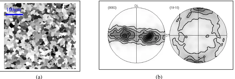
Thanks to SEM, the microstructure of the testing samples has been characterized using the EBSD technique. We have obtained a map of crystalline orientations (fig. 1a) of a studied area determined on the sample (central area of the sample with a surface of 800x800µm2). The EBSD analysis is performed with a step of 1µm (around 640000 points). Moreover, this technique permits to measure the highly pronounced texture of this material (fig. 1b), texture that is equivalent to the one observed on fuel cladding tubes, typical of rolled and recrystallized α-Zr alloys.

100µm

(a) (b)

Fig. 1: (a) crystalline orientations obtained by EBSD (b) Texture obtained on the same area (density 0.94, DL = rolling direction, DT = transverse direction)

(3)

Copyright © 2005 by SMiRT18 A macroscopical uniaxial tensile test at 200°C until a total strain of 2.5%, is performed in order to obtain the global behavior of the material for a representative temperature condition. Moreover, the samples are equiped with gold microgrids (step 2µm), deposited by micro-lithography on the surface before the tensile test, in order to obtain the residual displacement fields at the surface. Then, using a discrete derivation scheme [Allais,1994] on a 4µm gauge length we can obtain the residual strain fields in the microgrid plane. We can associate an uncertainty to this measure of 6.10-3. This does not allow to measure elastic strain, but it suits with our study because the uncertainty is small in comparison with the heterogeneity of the measured strains (0-10%).

2.2 Numerical simulation

2.2.1 Mesh and boundary conditions

The mesh is based on the gold microgrid. Each element of the mesh (cubic with 8 nodes and 8 Gauss points) corresponds with an element of the microgrid (size 2x2µm2) and is associated with the lattice orientation determined by EBSD. The mesh used consist of one layer of 3D elements having a small thickness compared with other dimensions.

The mechanical conditions on the boundaries that are used in this methodology are the displacements measured by microextensometry at the microgrid nodes, nodes that correspond to the mesh’s ones. On the upper and lower faces, boundary conditions consist of conditions of free surface. These conditions assume that the effect of underlying microstructure can be neglected if we only consider the strains at the surface of the sample, but this question has still to be clarified.

2.2.2 Crystalline constitutive law

For this material, at this temperature, the slip system activated are mainly prismatic (P<a>):

{

1010

}

1210

and pyramidal <a> (Pyr<a>):

{ }

1011 1210 . Two other slip systems, namely basal (B<a>):

{

0002

}

1210 and

pyramidal <c+a> (Pyr<c+a>):

{

1011

}

2113 , were times to times observed.

The constitutive equations describing the local behavior of the material has been implemented [Haddadi, 2003] and developed by M. Sauzay in the finite element code Cast3M® [Cast3M®, 2005]. It is an elasto-viscoplastic crystalline constitutive law, defined and used at first within the hypothesis of small perturbations. It can be described with the following relations. First we have the elasticity law:

Eq. 1

σ

&

=

K

(

ε

&

−

ε

&

vp

)

where

K

is the tensor of elasticity,

σ

&

the stress rate,

ε

&

and

ε

&

vpthe total strain and viscoplastic strain rates

respectively. The viscoplastic strain rate is given by:

Eq. 2 =

∑

ℜ

s s

s

vp _γ

ε& &

where s

ℜ

is the orientation matrix of system (s) with:

Eq. 3

(

)

s s s s

s= m ⊗n +n ⊗m

ℜ

2 1

and

γ

&

sthe shear strain rate on slip system (s). m_sis the slip direction of the system (s) and n_s the normal to its plan. The shear rate follows a law which presents a hyperbolic sinus. According to [Brenner, 2002] and following the works of [Delobelle, 1996] and [Masson, 1998], zirconium alloys’ behavior are better described with this kind of law than with classical ones.

Eq. 4

( )

s

n s s s s s τ τ τ γ

γ sinh sgn 0 0 ⎟ ⎠ ⎞ ⎜ ⎝ ⎛ =& &

where τs is the resolved shear stress on slip system (s). Each slip system is associated with a reference shear

rate s

0

γ& , a critical resolved shear stress

τ

₀s and a coefficient of stress sensibility ns. The hardening law is here

limited to a linear hardening:

Eq. 5

=

∑

k s sk s

_h

γ

τ

_&

0

_&

where hsk is the matrix of interaction between the slip systems. This matrix has been simplified by using:

(4)

Eq. 6 hsk=H0 Qsk

where H0 is the hardening parameter and Qsk is given by:

Eq. 7 Qsk=Qsk0 + (1-Qsk0)δsk

This implies that the hardening matrix is reduced to two values, one for diagonal terms expressing self-hardening, and one for off-diagonal terms expressing latent-hardening. This expression means that hardening (latent or self-hardening) does not depend on nature of the considered slip systems. The efficiency of such a description will be discuss later.

2.2.3 Optimization definition

The optimisation of the parameters of the constitutive law used in FEM simulation is done by minimization of a function based on the discrepancy between mechanical parameters (Σ and ε) obtained by experiments and those coming from numerical simulations. Indeed, at the local scale, a comparison is made on each point of the surface of the mesh between the in-plane strain tensor coming from FEM simulations (εsim) and the one coming from experiment (εexp).

The local discrepancy (EL) is defined as the average of a norm of the difference between the experimental strain tensor and the simulated one (Eq. 8).

Eq. 8

(

)

2

12 2 22

11 4

3

2 _∆_ε ₋_∆_ε ₊ _∆_ε =

L E

where

Eq. 9 ∆εij = εijexp - εijsim

At the macroscopic scale, the comparison is done between the values of stress measured during the experiment (

Σ

expi ) at a certain time (tj) (with for an uniaxial tensile test) and the average of the

stress coming from each Gauss point of the FEM simulation ( 0 exp exp=Σ =

Σyy xy

sim i

Σ

) during the loading for the same time (tj). The

macroscopic discrepancy (EM) is defined as the average of the difference between the experimental axial stress and the simulated one for different simulated steps (Eq. 10).

Eq. 10

( )

(

)

0 T M t N t E T = ∆Σ =

∑

where

Eq. 11 N

(

∆Σ

( )

t

)

= ∆Σ + ∆Σ + ∆Σ2_xx 2_yy 2_xy

and

Eq. 12

( )

t

( )

t

sim

( )

t

i i

i

=

Σ

−

Σ

∆Σ

exp

Those two comparisons compose the function that we want to minimize in order to optimize the parameters of the constitutive law used.

Nevertheless, such a method implies a good description of the loading path during the FEM simulations.

3. STUDY OF BOUNDARY CONDITIONS 3.1 Limitations observed

3.1.1 Experimental boundary conditions

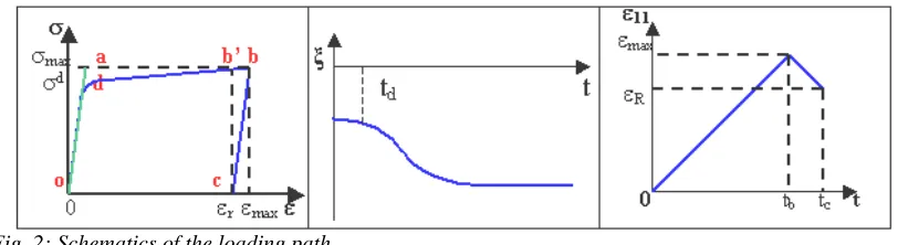
For experimental reasons (macroscopical tests), the picture of the deformed microgrid is done when the sample is unloaded. This does not permit to know the local displacement fields corresponding to the state referred as b on the loading path (fig. 2). So experimentally we can only reach the residual displacement fields (state c, fig. 2). Applying those displacements as boundary conditions would get to a pseudo-state b’ that would not be appropriate. So for the simulation, we have to introduce an additionnal field, that would help describing the state b and the evolution through the state c. This field has to be compatible and admissible. It is determined by a numerical simulation in the elastic domain (see further explanations in 3.2.1).

(5)

Fig. 2: Schematics of the loading path

3.1.2 Evolution of the boundary conditions

Making a FEM simulation by applying a linear and proportional loading path as a function of time, in order to describe the path from o to b, implies a constant strain ratioξ=<εyy>prescribed/<εxx>prescribed during the whole

loading. Now experimentally, for a uniaxial tensile test, this ratio evolves during the loading (fig. 2, evolution according to the current state, elastic or plastic).

So, prescribing a constant strain ratio, equal to the ratio of residual measured strains (around -0.7, measured experimentally), gives rise to transverse stresses, especially in the elastic state where this ratio is experimentally around –0.36.

Consequently, we have to face this problem of description of the loading path. As the mechanical parameters we want to identify are the ones that define the onset of plasticity, we have to be sure that the loading path is well described at the beginning of the loading.

3.2 Proposals

3.2.1 Description of the boundary conditions

Different propositions have been compared in order to determine a realistic loading path.

The additional field on the mesh outline is calculated thanks to a simulation with an elastic behavior using a uniaxial stress loading up to the maximal stress observed during the experiment. For this simulation, the constitutive law that is used is the one described earlier which is crystalline and permits to take into account the elastic anisotropy of the material. The calculated additional field is the result of the simulation of the loading path from o to a on fig. 2.

Then, the displacements applied as boundary conditions are at the state b the addition of displacements measured by microextensometry and displacements coming from the simulation described above (path o to a). The path b to c is simulated by an unloading to the experimental measured displacements.

3.2.2 Evolution of the loading path

First of all, the boundary conditions coming from the experiment will be referred as URmax, and the

additional boundary conditions coming from the numerical simulation (path o to a) will be referred as UEmax.

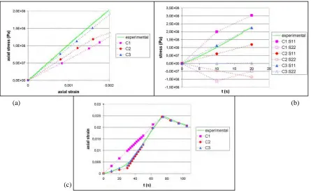
The first proposal consists in a linear and proportional loading path where displacements are applied within the way described in fig. 3a.

Eq. 13 U(t) = (UEmax + URmax) * f(t) Eq. 14 U(t) = (UEmax + URmax) * h(t) for t

∈

[0 tb]

Eq. 15 U(t) = UEmax * d(t) for t∈[tb tc]

(a) (b)

Fig. 3: (a) first studied evolution of loading path referred as C1 (b) second studied evolution of loading path referred as C2

(6)

Copyright © 2005 by SMiRT18 Without regards to the stress level obtained in the plastic state, it is clear that the description of the elastic state is not in agreement with the evolution of the loading path. Indeed, on fig. 4a the apparent Young’s modulus obtained with this evolution is too weak (61GPa) compared with experimental results (91GPa).

This comes from the biaxial tension induced by the proportional loading path. One can observed on fig. 4b, for the evolution C1, that in the elastic state, the transversal stress component S22 is not equal to zero. Moreover, one can also observed that using a linear evolution for the loading path is a poor description of the evolution of the axial strain versus time (fig. 4c).

(b)

(c) (a)

Fig. 4: Comparisons between experiments and results coming from numerical simulations (a) Axial stress-strain curves (b) axial (S11) and transversal (S22) stresses versus time (c) axial strain versus time

A first improvement, referred as C2, consists in using a proportional but non linear evolution of the loading path as a function of time. In fact, to have the same variations as those induced by the control of the tensile test with the cross head displacement, the evolution includes a change in the loading rate.

This evolution still presents the problem of proportionality (problem of non-uniaxial loading, fig. 4a and fig. 4b), the evolution of axial strain with time is better than before (fig. 4c).

The last improvement, referred to as C3 (fig. 5), gives a non-proportional evolution of the loading path [Gélébart, 2004], where f and g are functions that give the kinetic of the loading and where σdexp and td

correspond to the axial stress and the time at the yield surface.

Eq. 16 U(t) = UEmax * f(t) + URmax * g(t)

Fig. 5: Third studied evolution of loading path, referred as C3

(7)

Copyright © 2005 by SMiRT18 This solution, with a non-proportional evolution of the loading path, gives a more realistic description of the elastic state: the stress state is uniaxial, the elastic modulus is well described as well as the evolution of strain as a function of time (fig. 4). So this way of applying the boundary conditions seems to be more realistic than a proportional one, commonly used, and allows to be confident to identified parameters describing the yield locus.

4. APPLICATIONS

4.1 Experimental boundary conditions

First, a comparison has been made between experiments and simulations using two kind of boundary conditions, experimental one and homogeneous strain ones. Homogeneous strain boundary conditions are the ones that gives, for an homogeneous material, an homogeneous strain response, on the whole mesh, equal to the macroscopic experimental one. The boundary conditions are given in displacements and are on the outline of the mesh:

Eq. 17 U(M) = E.M

where E is the macroscopic strain tensor, M the point where the condition is applied and M its coordinates. The parameters used for this comparison are for s

0

γ

_&

, ns and Q0s, those determined by R. Brenner (2002) for

creep test on a sample of Zircalloy-4, and the others (τs0 and H0) are just estimated, keeping in mind the

experimental observations on relative ease of activation of the different slip systems. They are reported on table 2.

Slip system

γ

&

0(s-1) n Q

0 _τ

0 (Mpa) H0 (MPa)

P<a> 1.10-7 3 2 20 100

Pyr <a> 1.10-7 7 2 40 100

B<a> 1.10-7 7 2 80 100

Pyr<c+a> 1.10-7 7 2 80 100

Table 2: Parameters used for comparing results with homogeneous strain boundary conditions and results with experimental ones.

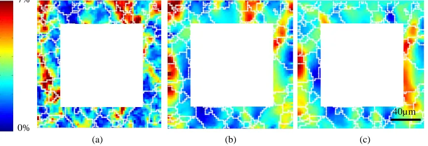
In order to look at this effect the comparison is made between the experiment and the simulations on the two first layers of grains because this effect vanishes with the distance to the boundary.

Even if the parameters used for these simulations are subjectively chosen, you can already see that the results given by a simulation using experimental boundary conditions seems to be better than those given by a simulation using homogeneous strain boundary conditions (fig. 6).

First of all, the macroscopic discrepancy is higher with homogeneous strain boundary conditions (4.2 MPa) than with experimental boundary conditions (3.7 MPa). The axial strain field obtained with homogeneous strain boundary conditions is less heterogeneous than the one obtained with experimental boundary conditions. The localization is not high enough and not enough numerous with homogeneous strain boundary conditions. Moreover, the local discrepancies calculated in both cases are of 1.9% and 2.3% for experimental and homogeneous strain boundary conditions respectively.

7%

0%

(a) (b) (c)

40µm

Fig. 6: Comparison of the axial strain field (a) measured by microextensometry and calculated with (b) experimental boundary conditions and (c) homogeneous strain boundary conditions

(8)

4.2 Identification of material parameters

A way for identifying constitutive law parameters is to use an automatic software that minimizes a function describing the distance between measured and computed values at the desired scales and that depends on the parameters to identify.

Such a procedure has not been carried out yet. The identification that is done in this paper uses as parameters

τ

0p<a> and αi, where:

Eq.18

=

_p_<_a_>

i i

0 0

τ

α

As the automatic procedure is not performed yet, the identification described in this paper is restricted to the identification of two parameters

τ

0p<a> and αpyr<a>.

A pre-identification is performed which consist in identifying on the axial stress at the end of the loading, the other parameters being the ones listed in table 3.

> <a p 0

τ

Slip system

γ

&

0(s-1) n Q

0 _α

H0 (MPa)

P<a> 1.10-7 3 2 1 50

Pyr <a> 1.10-7 7 2 1-6 50

B<a> 1.10-7 7 2 6 50

Pyr<c+a> 1.10-7 7 2 6 50

Table 3: Parameters used for the pre-identification

For each value of αpyr<a>, < > is identified. The evolutions of E

a p 0

τ

M

and EL as functions of αpyr<a> are used

to find out the optimal value of αpyr<a> and its associated < >.

a p 0

τ

As

τ

0pyr<a> is known to be higher than and lower than >

<a p 0

τ

b<a>

0

τ

and , the parameter

α

> + <c a pyr 0

τ

pyr<a> moves only between 1 and 6. The criterion used for identification is the discrepancy between the

experimental and the calculated axial stress at the maximal load (state b on fig. 2). The parameter is identified when this discrepancy is lower than 1% of the maximal experimental axial stress. This criterion is usually reach with 2 to 4 iterations.

4.3 Application

The tensile test used for identification has been performed on a sample with a tensile test direction parallel to the rolling direction.

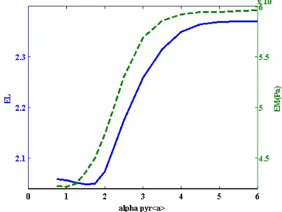
Fig. 7: Evolutions of macroscopic and local discrepancies

The evolutions of the local discrepancy ,EL ( ), and the macroscopic one, EM ( ), with αpyr<a> show

well defined minimums (fig. 7). The local discrepancy exhibits a minima for the value 1.5 of αpyr<a>, and the

macroscopic one for the value 1. The optimal set of parameters that has then been determined is given in table 4.

(9)

P<a> 1 31.4 Pyr <a> 1.25 39.2

Table 4: Identified parameters considering αb<a>=αpyr<c+a>=6, rolling direction.

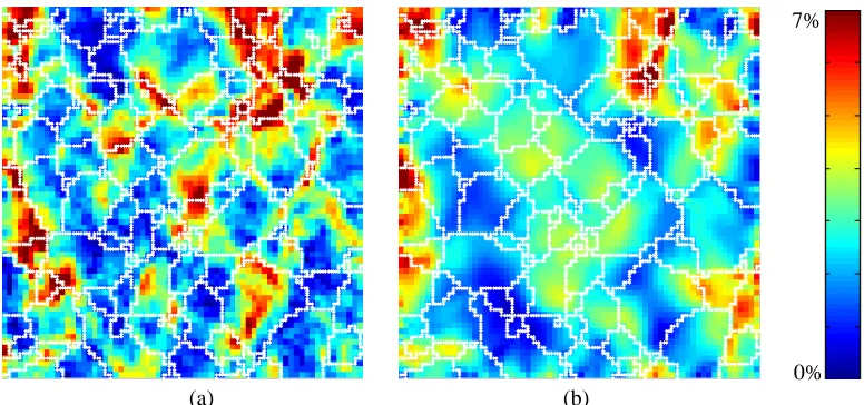
Then, the comparison between the measured local strain field and the calculated one (fig. 8) shows that even if the strain localization is still too weak, the global scheme of localization is agreed.

0%

7%

(a) (b)

Fig. 8: Comparison between the axial strain field for a tensile test direction parallel to the rolling one (a) measured by microextensometry and (b) calculated by finite element method (DOF:14000 ).

5. CONCLUSIONS AND PROSPECTS

An identification method has been set up for the parameters of a constitutive law, using a coupling between EBSD, microextensometry and finite element simulation. It has been validated on an industrial material and shows a good potential even if some points are still to be clarified.

Indeed, inquiries will soon be performed in order to verify several hypothesis that could explain the differences observed between results coming from experiments and simulations. First, even if the macroscopic strain is equal to 2.5%, the local strain can rich more than 7%. It implies the use of large deformations and large rotations for the finite element simulation that has not been performed here.

Then, the constitutive law used for these simulations is described with a linear hardening. This does not seem to be good enough for this material hardening description. A new hardening law will be tested using a non linear hardening, based on physical parameters such as dislocation densities.

Tests on bigger areas have also to be done in order to test the size of the Representative Volume Element. Finally, an inquiry has begun in order to look at the influence of the third dimension on result obtained on surface.

Yet, the study performed on the evolution of the loading path already shows that using a linear and proportional loading path implies a bad description of the loading. The last proposal that has been shown in this paper gives good results for the description of the beginning of the loading, which means a good description of the onset of plasticity that is significant for the identification of parameters such as critical resolved shear stresses.

ACKNOWLEDGEMENT

This work was funded by the joint research program “SMIRN” between EDF, CEA and CNRS.

(10)

C.N. Tomé, P.J. Maudlin, R.A. Lebensohn, G.C. Kaschner, (2001), Acta mater., vol. 49, pp. 3085-3096. C. Pujol, (1994), PhD thesis, Ecole Nationale Supérieure des Mines de Paris, France.

H. Haddadi, S. Héraud, L. Allais, C. Teodosiu, A. Zaoui, (2003), A « mumerical mesoscope » for the investigation of local fields in rate-dependent elastoplastic materials at finite strain, Symposium IUTAM « Computational Mechanics of Solid Materials at Large Strains », Ch. Miehe (ed), Kluwer Academic Pub., The Netherlands, pp. 311-320.

P. Doumalin, M. Bornert, J. Crépin, (2003), Mécanique & Industries, vol. 4, Issue 6, pp. 607-617.

L. Allais, M. Bornert, T. Bretheau, D. Caldemaison, (1994), Acta. Metall. Mater., vol. 42, n°11, pp. 3865-3880. Cast3M®, (2005): http://www-cast3m.cea.frT

R. Brenner, J. L. Béchade, O. Castelnau and B. Bacroix, (2002), Journal of Nuclear Materials, vol. 305, Issues 2-3, pp. 175-186.

P. Delobelle, P. Robinet, P. Geyer, P. Bouffioux, (1996), Journal of Nuclear Materials, vol. 238, Issues 2-3, pp. 135-162.

R. Masson, (1998), PhD thesis, Ecole Polytechnique, France.

L. Gélébart, J. Crépin, M. Dexet, M. Sauzay, A. Roos, (2004), Journal of ASTM International, vol. 1, Issue 9.

Identification of Constitutive Laws by Inverse Method Based on EBSD, Microextensometry and Finite Elements Simulations. Application to Zirconium Grade 702