Hyperfast Correlated Dynamics of Radiation Damage and Recovery in Materials.

ABSTRACT

XIAOJUN, MEI. Hyperfast Correlated Dynamics of Radiation Damage and Recovery in

Materials. (Under the direction of Dr. Jacob Eapen.)

The response of solid-state materials to radiation is governed through a host of mechanisms that have time scales ranging from femtoseconds to seconds and years. Metastable liquid-like regions that typically last for several picoseconds and more are commonly observed in ultra-fast experiments and simulations. In this investigation, we make quantitative predictions on correlated dynamical motion of the atoms as the liquid-like state is formed and condensed following an ion or neutron impact. Simulations on three materials – copper, silicon and argon – that have very different bond structures reveal an anisotropic and heterogeneous dynamical structure. Of utmost importance are the dynamical correlations during the recovery period, which corresponds to the condensation of the liquid-like state.

Using molecular dynamics simulations and with the appropriate non-equilibrium shock physics formalism, the dynamical metrics of the liquid-like state are evaluated through the density correlator and van Hove self-correlation function, as well as through defect, thermodynamic and hydrodynamic field data, following a confined ion/neutron impact. These correlation functions can also be experimentally accessed or inferred from the state-of-the-art ultrafast pump-probe experimental methods. The hopping mechanism from the van-Hove self-correlation, the fractal-like condensation and the fast decay of the density correlator attest to a rapid defect recovery in copper. In contrast, silicon portrays dynamically heterogeneous regions that resist recovery to the underlying lattice structure, and exhibits a non-decaying density correlator that is strikingly analogous to that of a supercooled liquid.

Hyperfast Correlated Dynamics of Radiation Damage and Recovery in Materials

by

Xiaojun Mei

A dissertation submitted to the Graduate Faculty of

North Carolina State University

in partial fulfillment of the

requirements for the degree of

Doctor of Philosophy

Nuclear Engineering

Raleigh, North Carolina

2013

APPROVED BY:

_______________________________ ______________________________

Dr. Jacob Eapen Dr. K. L. Murty

Chair, Advisory Committee

Member, Advisory Committee

_______________________________ ______________________________

Dr. Mohamed Bourham Dr. Keith Gubbins

DEDICATION

To my dear parents.

To my beloved wife, Mengying.

BIOGRAPHY

Born in Chaohu, China in 1987, Xiaojun Mei received his Bachelor’s degree in Physics from the

University of Science and Technology, China in 2008. Following his graduation, he joined the

Department of Nuclear Engineering at the North Carolina State University in Fall 2008. Since

then he has been focusing on molecular simulations of radiation damage and recovery in

materials using statistical-mechanical principles under the supervision of Dr. Jacob Eapen. His

deep interest in mathematical and statistical methods has motivated him to purse graduate studies

in the same area; he received a Master of Science degree in Statistics from the Department of

Statistics in 2011. He intends to work in the field of computational and statistical sciences in his

ACKNOWLEDGEMENTS

At the outset, I would like to express my heartfelt appreciation to Prof. Jacob Eapen for his

unstinting support and guidance throughout my graduate studies. He has been very patient and

encouraging during the time I spent under his supervision.

I am immensely indebted to my advisory committee members – Prof. K. L. Murty, Prof.

Mohamed Bourham and Prof. Keith Gubbins, for their insightful comments and encouragement

on my dissertation work.

I would like to record my sincere gratitude to all the members of Prof. Jacob Eapen’s RADIANT

research group for their support and refreshing sense of optimism. In particular, I would like to

thank Dr. Prithwish Nandi, who assisted me on defect analysis and for reviewing part of my PhD

dissertation. It was a great pleasure to share the stimulating company of Dr. Walid Mohamed,

Ajay Annamareddy, Anant Raj, Jin Wang and William Lowe.

My sincere appreciation goes to all who helped me at the department – in particular, I want to

thank Ms. Ganga Atukorala, Ms. Hermine Kabbendjan and Mr. Robert Green for helping me with

the curricular and administrative matters over the last five years.

Finally, I would like to express my love and gratitude to my wife for her kindness,

TABLE OF CONTENTS

LIST OF FIGURES ... vii

Chapter 1. Introduction ... 1

1.1 Radiation Applications ... 1

1.2 Dynamical Characteristics of Early Radiation Interactions ... 2

1.3 Motivation for Current Research ... 4

Chapter 2. Theory ... 6

2.1 Liouville Equation ... 6

2.2 Time Correlation Functions ... 7

2.2.1 Space-Time Correlation Functions ... 9

2.2.2 Correlators in Reciprocal Space ... 11

2.3 Non-Equilibrium Microscopic Thermodynamic Variables and Fluxes ... 13

Chapter 3. Molecular Dynamics (MD) Simulations ... 15

3.1 Introduction ... 15

3.2 Interatomic Potentials for Equilibrium States ... 16

3.3 Interatomic Potentials for Non-Equilibrium States ... 19

3.4 Propensity and Displacement in Isoconfigurational Ensemble ... 21

3.5 Non-Equilibrium MD Radiation Cascade Simulations and Boundary Control ... 23

3.6 Field Construction ... 25

Chapter 4. Liquid-Liquid Phase Transition in Silicon ... 26

4.1 Introduction ... 26

4.2 Time Correlators and Molecular Dynamics Simulations ... 27

4.3 Dynamic Transitions from Viscosity ... 29

4.4 Structural Motifs for the Dynamic Transitions ... 31

4.5 Decoupling of Stress, Density and Energy Correlators ... 33

4.6 Collapse of Dynamical Heterogeneity ... 36

4.7 Concluding Remarks ... 39

Chapter 5. Radiation Damage and Recovery ... 40

5.2 Mean Displacement of the PKA and its Neighbors ... 41

5.3 Non-Equilibrium Energy Distribution from Superpositioning of Two Equilibrium States . 45 5.4 Radial Distribution Function following Radiation ... 50

5.5 Interplay between the Shock Fields and the Transient Defects ... 52

5.6 Stress and Temperature Relaxations ... 61

5.7 Dynamical Heterogeneity via the Evolution of Time-Resolved Van Hove Self-Correlation ... 65

5.8 Displacement Distribution ... 67

5.9 Dynamical Recovery ... 71

Chapter 6. Conclusions ... 75

LIST OF FIGURES

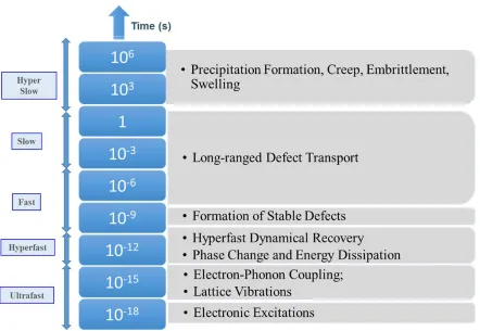
Figure 1.1 Timescales for materials response in a radiation environment. This dissertation focuses on statistical-mechanical analyses of the dynamics during the early interaction processes, which are characterized by phase change, energy dissipation and dynamic defect recovery at the hyperfast timescales. ... 3

Figure 3.1 An isoconfigurational ensemble ... 21

Figure 3.2 (Left) MD simulation box depicting the primary knock-on atom (PKA). An impulse along the (1 0 0) direction, which is parallel to the x-axis, is given to the PKA. (Right) An ‘inner box’, which is further divided into ‘fore’ and ‘wake’ regions, is employed to evaluate the local dynamical and structural changes near the PKA. ... 23

Figure 3.3 Method of temperature control at the boundary layers ... 24

Figure 3.4 Field construction on a plane normal to radiation impact ... 25

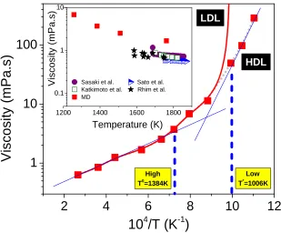
Figure 4.1 Viscosity of supercooled Si and two transition temperatures marked as “High’ (≈1384 K) and ‘Low’ (≈1006 K). The HDL–HDL dynamic crossover is validated with observations on cage dynamics (Figure 4.2), attendant decoupling in density/stress/energy relaxations (Figures 4.3 and 4.4), and the evolution of dynamic heterogeneity (Figures 4.5 and 4.6). (Inset) A comparison of MD simulation results with experimental data [134-137] showing a modest over–prediction with SW potential. ... 29

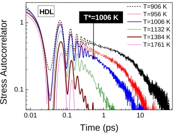
Figure 4.2 Stress autocorrelators (arbitrary units) for HDL at different temperatures. ... 30

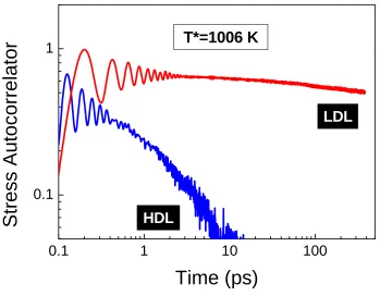
Figure 4.3 Comparison of stress autocorrelators (arbitrary units) for HDL and LDL at 1006K. ... 31

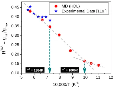
Figure 4.4 Wendt and Abraham ratio (RWA) for HDL at different temperatures. For LDL, RWA drops to 0.027 at 1006K (not shown). ... 32

Figure 4.5 The ratio of structural relaxation time with a wavevector of 0.34 Å-1 _{to the viscous}

relaxation time (τα/τψ) for HDL. (Inset) VDOS for HDL at 1006K showing two prominent frequencies, 4 THz and 15 THz. ... 33

Figure 4.6 Density and energy correlators at 956K for different wavevectors. A wavevector of value 2.78 Å-1 _{is near the first peak in the structure function at 1540K... 35}

Figure 4.7 Variation of energy (E) relaxation time (τε) and density (F) relaxation time (τα) with temperature for HDL. ... 36

times τ = [0.2, 0.5, 4.5] ps (first panel from top ), (ii): HDL at 1006 K evaluated at different times τ = [20, 60, 460] ps (second panel from top), (iii): LDL at 1006 K evaluated at different times τ = [20, 60, 460] ps (third panel from top), and (iv): crystal at 1006 K (fourth panel from top)

evaluated at different times τ = [20, 60, 460] ps... 37

Figure 4.9 (top panel): Propensity distributions for HDL (left) and LDL (right) at 1006 K. (bottom panel): Temporal variation of propensity for HDL, LDL and solid (crystal) at 1006 K. ... 38

Figure 5.1 Temporal scaling behavior of the PKA. EPKA = 3 keV for Cu and Si, and 100 eV for Ar; the ratio of PKA energy to the mean displacement energy is O(100). ... 41

Figure 5.2 Displacement scaling with PKA energy ... 42

Figure 5.3 Mean displacements of PKA neighbors in copper. EPKA = 3 keV. ... 43

Figure 5.4 Mean displacements of PKA neighbors in silicon. EPKA = 3 keV ... 44

Figure 5.5 Mean displacements of PKA neighbors in argon. EPKA = 100 eV. ... 44

Figure 5.6 The evolution of the non-equilibrium energy distribution for Cu, Si and Ar at different times. The symbols connote data derived from the cascade MD simulations and the line denotes the prediction from the two-temperature (T, Θ) model. EPKA = 3 keV for Cu and Si, and 100 eV for Ar. ... 47

Figure 5.7 Bi-modal temperature variation for Cu (T – line, Θ – symbol). EPKA = 3 keV. ... 48

Figure 5.8 Bi-modal temperature variation for Si (T – line, Θ – symbol). EPKA = 3 keV. ... 48

Figure 5.9 Bi-modal temperature variation for Ar (T – line, Θ – symbol). EPKA = 100 eV. ... 49

Figure 5.10 Displaced atoms as a function of time with the peaks appearing at Θ≈T indicating that the dynamic recovery advances under local thermodynamic equilibrium. ... 50

Figure 5.11 RDF of Cu following radiation. EPKA = 3 keV. ... 51

Figure 5.12 RDF of Si following radiation. EPKA = 3 keV. ... 51

Figure 5.13 RDF of Ar following radiation. EPKA = 100 eV. ... 52

Figure 5.14 The temporal evolution of the spatial fields for Cu in the yx plane. The radiation impact is along the x direction (shown by an arrow in the top-left sub-panel) at the center of the plane. EPKA = 3 keV. ... 53

Figure 5.16 The temporal evolution of the spatial fields for Si in the yx plane. The radiation impact is along the x direction at the center of the plane. EPKA = 3 keV. ... 56

Figure 5.17 The evolution of spatial fields in the yz plane (normal to the knock) for Si. EPKA = 3

keV. ... 57

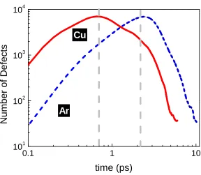
Figure 5.18 Defect evolution in Si and Cu. EPKA = 3 keV for Cu and Si. ... 58

Figure 5.19 The temporal evolution of the spatial fields for Ar in the yx plane. The radiation impact is along the x direction at the center of the plane. EPKA = 100 eV... 59

Figure 5.20 The evolution of spatial fields in the yz plane (normal to the knock) for Ar. EPKA =

100 eV. ... 60

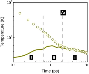
Figure 5.21 Relaxations of temperature (top), and pressure (bottom) following radiation impact. The left and right panels correspond to the wake region behind the PKA and the fore region ahead of the PKA, respectively. Red solid curve is for Cu, blue short dash curve is for Si, and dark yellow dash dot curve is for Ar. ... 62

Figure 5.22 Directional temperature relaxations. Blue solid curve is for , red short dash and dark yellow solid curves are for , and , respectively. ... 63

Figure 5.23 Directional Pressure (Diagonal Stress) relaxations. Blue solid curve is for , red short dash and dark yellow solid curves are for , and , respectively. ... 64

Figure 5.24 van Hove self-correlation function for Cu (top), Si (middle) and Ar (bottom) following radiation impact. The left and right panels correspond to the wake region behind the PKA and the fore region ahead of the PKA, respectively. The exponential tail in the fore regions signifies a dynamically heterogeneous recovery; the peaks in the tail indicate hopping of atoms. The grey broken lines in Cu and Ar (fore) panels indicate the nearest neighbor positions. ... 66

Figure 5.25 Directional displacement distribution in the fore region following radiation impact. The left panel depicts the displacement in the knock (x) direction while the right panel shows the displacement in a transverse (y) direction. ... 68

Figure 5.26 Directional displacement distribution in the wake region following radiation impact. The left panel depicts the displacement in the knock (x) direction while the right panel shows the displacement in a transverse (y) direction. ... 69

Figure 5.28 Most mobile (top 20%, red) and most immobile (bottom 20%, green) atoms at

different times for Cu and Si following radiation impact. ... 72

Figure. 5.29 Time-resolved density correlator for Cu following radiation impact. ... 73

Figure. 5.30 Time-resolved density correlator for Si following radiation impact. ... 73

Figure. 5.31 Time-resolved density correlator for Ar following radiation impact. ... 74

Figure. 5.32 Time-resolved density correlator for the equilibrium state. ... 74

Chapter 1. Introduction

Radiation is ubiquitous in nature; it is the most dominant mode of energy transport in the universe. Radiation includes electromagnetic waves or photons, as well as particles with finite rest mass such as electrons, ions and neutrons. When radiations interact with condensed matter, its atomic structure gets altered. Prolonged exposure to radiation generally results in the formation of macroscale defects that adversely affect the performance of materials. Several energy-related applications where radiation plays an active role are briefly reviewed next.

1.1 Radiation Applications

(i) Nuclear Energy: High energy neutrons, of the order of 1 MeV, are generated from fission process that takes place in the fuel elements of nuclear reactors. Because they are electrically neutral, neutrons have a large mean free path that is of the order of 1 centimeter. Thus fast neutrons escape from the core of the nuclear reactors and interact with the structural elements such as the reactor or pressure vessel and piping units. Over time the structural elements degrade and lose their integrity [1]. The fuel, after its serviceable lifetime in a reactor, is stored as spent fuel, first under water and then in dry storage casks. Because of radioactive decay, the spent fuel matrix is continuously subjected to β radiation from the fission products and α radiation from the actinides. A fundamental understanding of the radiation damage processes and those which aid in recovery or healing is essential to develop radiation and accident tolerant materials for nuclear energy. A comprehensive account of radiation damage in nuclear materials is given in [2].

noted by Freund and Suresh [7], attendant residual stresses put a limit on to quality and reliability of thin films even when they are not designed or required to be load-bearing. It therefore, remains a challenge to generate high quality films at a faster rate without the detrimental effects of anisotropy, imperfections and the attendant intrinsic, thermal and interfacial stresses. A fundamental understanding of the energy transfer mechanisms, which can control the surface transport and recombination is thus required [8].

(iii) Solar Energy: Even though energy density from solar radiations is considerably lower than that in nuclear radiations, solar cells are severely tested by rapidly varying and large temperature loads [9]. The highest photovoltaic efficiency (of approximately 35%) has been attained with epitaxially grown compound semiconductor multi-junction structures that collect light across the solar spectrum. However, these compounds are also extremely sensitive to material defects, which are generated during material synthesis as well as from radiation exposure to sun. Solar concentrators, which are designed to operate at temperatures as high as 3000 °C [9, 10], present new materials-related challenges. Space-based solar systems are further bombarded by fluxes of electrons and protons trapped in the electromagnetic field of earth [11, 12]. Thus there is a demonstrated need to discover, design and synthesize new materials for solar energy systems that are intrinsically insensitive to defects [9].

1.2 Dynamical Characteristics of Early Radiation Interactions

harmonic light experiments and molecular dynamics (MD) simulations [29]; in the first stage homogeneous melting takes place, which lasts for few picoseconds, followed by a relatively longer period of 25-30 ps, during which the melt interface propagates into the bulk. Such staggered melt processes are also identified in several molecular simulations [16, 17]. Shock waves are instrumental in the energy transfer – during the incipient isochoric heating from the incident photons, compressive shock waves are generated. On reflection from the free surface the compressive wave becomes a tensile or rarefaction wave that propagates through the melt region and causes cavitation (voids) as well as spallation/fragmentation [16, 17, 28].

Figure 1.1 Timescales for materials response in a radiation environment. This dissertation focuses on statistical-mechanical analyses of the dynamics during the early interaction processes, which are characterized by phase change, energy dissipation and dynamic defect recovery at the hyperfast timescales.

fuel and structural elements in nuclear reactors over time. While laser energy is transferred through the electronic excitation and the subsequent electron-phonon coupling, the ions and neutrons can transfer their kinetic energy directly to the nucleus. A two temperature model that explicitly accounts for the ion and electron temperatures, therefore, is typically employed to describe the energy absorption and dissipation processes [16, 25] in laser interactions; the electronic coupling and transport, however, is conveniently neglected for ion and neutron interactions, especially at low energies [38, 39].

Despite the differences in the energy transfer mechanisms, ion and neutron interactions share similar dynamical features to those of the laser interactions. Due to the rather low atomic number density or flux, ions and neutrons interact with one target nuclei at a time generating a three dimensional thermal spike lasting several picoseconds, following an ultrafast ballistic period. In MD simulations, the primary knock-on atom (PKA) mimics the nucleus that absorbs the ion/neutron energy; it transfers the energy to the surrounding atoms through a series of cascading collisions. Thermal spikes, which are created at energies 1 keV and higher [21], introduce a superheated disordered region that is often likened to a liquid state, an analogy stemming from the similarities in the structure and diffusional properties of the cascade core region [40]. Induced stresses and morphology changes during the thermal spike period from ion bombardment are attributed to the radiation-induced viscous relaxation in metallic and amorphous thin films [22, 41]. It is now established that the stress evolution is governed by the initial stress state, and there is a competition between tensile and compressive stresses, the former generated by the liquid-like regions and the latter by the accumulation of ion-induced interstitials [13]. Anisotropic diffusion, depending on the stress states, and non-trivial coherent displacement of atoms are also observed in thin films following ion irradiation [13, 42].

1.3 Motivation for Current Research

molecular dynamics (NEMD) simulations. However, most simulations in the past have focused on the formation and identification of defects that arise in a radiation environment. In this work, we make quantitative predictions on correlated dynamical motion of the atoms as the liquid-like state is formed and then condensed following an ion or neutron impact. Of utmost importance are the dynamical correlations during the recovery period, which determine the final defected state. The knowledge of the spatio-temporal characteristics immediately following radiation will be immensely valuable in designing accident and radiation tolerant materials for nuclear energy applications as well as for optimizing materials processing methods that use a radiation source.

Chapter 2. Theory

A central focus of the current work is to develop statistical-mechanical analysis methods for describing the materials response following radiation at the hyperfast timescales. This chapter discusses the theory of correlation functions that are used to characterize the dynamical response.

2.1 Liouville Equation

A 6N-dimensional phase space can be constructed from the 3N spatial coordinates and 3N momentum coordinates [44-49] for a system of N particles. A point in the phase space completely specifies the microscopic dynamical state and when the phase points become infinitely dense, there will be a continuum of phase points. The distribution function given by [50]

, , … , , , , … , ≡ , , _(2.1)

describes the fraction of phase points in an infinitesimal element of the phase space. From the conservation property of the distribution function, the evolution equation of the phase points can be expressed as [50]

⋅ _(2.2)

where u denotes the time derivative of the momenta and spatial coordinates, and is given by

, , … , , , , … , _(2.3)

In a conservative system, the distribution function is a constant along a trajectory in the phase space. Using Hamilton’s equations of motion, the following can be derived [50].

, _(2.4)

, 0 _(2.5)

Where H denotes the Hamiltonian – the sum of the potential and kinetic energies in the absence of external fields, and PB refers to Poisson bracket, which is given by

, ≡ _(2.6)

The Liouville equation can be also written as [50]

(2.7)

where L is the Liouville operator, which in Cartesian coordinates is given by

≡ _(2.8)

where and are the gradients with respect to spatial and the momentum coordinates

respectively. Fk is total force on the kth particle. The formal solution to the Liouville equation is given

by [50]

, , e , , 0 _(2.9)

2.2 Time Correlation Functions

The correlation function of two dynamical variables A and B is given by [51]

≡ ∗ _{≡ 〈} ∗_〉

(2.10)

only the differences in time – also known as the stationary property. The correlation function can now be written as [51]

∗

(2.11)

∗

(2.12)

∗

(2.13)

∗

(2.14)

Without loss of generality, τ can be set to zero. Then the correlation function can be written as

≡ 0 ≡ 〈 0 〉 _(2.15)

where the pointed brackets denote the ensemble average. When the same variable is considered, the resulting expression becomes the auto-correlation function

≡ 0 ≡ 〈 0 〉 _(2.16)

Originally developed by Boltzmann and Maxwell, the ergodic hypothesis postulates an equivalence between the ensemble average and the time average of an observable. It is expressed as

≡ 0 ≡ 〈 0 〉 ⇔ lim

→

1

0 _(2.17)

2.2.1 Space-Time Correlation Functions

The density field at a spatial point r and at a time t can be expressed as [50, 53]

, _(2.18)

The above describes the local density in terms of an infinitesimal region of space at r measured at time t. While the number of atoms entering and leaving the small volume is fluctuating, the total number of atoms in the system is conserved. To describe the fluctuations and structural probabilities from a macroscopic point of view, a density-density time correlation function can be constructed [47, 54, 55]

, ≡1〈 , , 0 〉

1〈 0 〉

(2.19)

The function above is also known as the van Hove correlation function, where is the Dirac delta and the angular brackets represent the time average. , is a dynamic quantity that is proportional to the probability of an atom being is at position r at time t given that an atom was at the origin 0 at initial time 0. van Hove correlation function can be divided into two parts [53]. Terms having give the self-correlation function , [50], for which the atom at , is the same atom that occupied at the origin 0, 0 . The terms having yield the distinct correlation function

, , for which the atom at , differs from the atom that occupied at the origin 0, 0 . Thus, the van Hove correlation function can be rewritten as [53]

, , , _(2.20)

The self-correlation function, also known as van Hove self-correlation function, is formally defined as

, 1〈 0 〉

(2.21)

, 1 _(2.22)

At long times and large distances, the position of an atom is unrelated to its original position and therefore, the atom is equally probable to be found anywhere in the system. From the above normalization we can find the value which is seen to collapse from δ (at 0) to zero. During this period, the shape of self–van Hove correlation function may be assumed as Gaussian-like (under equilibrium conditions). We shall discuss more on the variation of the shapes of van Hove correlation function in the later chapters of this dissertation.

The distinct correlation function, also known as the distinct van Hove correlation function, is defined as [50, 53]

, 1〈 0 〉

(2.23)

The normalization is given by

1

, 1 1 _(2.24)

, 0 is proportional to the radial distribution function and given by [53]

, 0 _(2.25)

At long times and large separations when the position of one atom is unrelated to the earlier position of another atom [53]

→ , → , (2.26)

In the analysis of radiation dynamics, we employ van Hove self-correlation function as a metric to monitor the dynamical characteristics of the formation of disordered zones and the dynamical recovery to a defected state. It is well-known that Gs(r,t) is related to the self-diffusion of the atoms

[52]; very recently, however, it has been established that Gs(r,t) is a reliable indicator for dynamical

atoms in highly frustrated states, typically associated with glassy and supercooled systems [43, 56-59]. Interestingly, the exponential decay in Gs(r,t) – the signature for the presence of faster moving

atoms – is also observed in jammed conditions such as in granular media, as well as in foams and colloids [60, 61]. Thus, time-resolved Gs(r,t) is an excellent metric to assess whether materials

deform and recover in a dynamically heterogeneous manner under radiation.

2.2.2 Correlators in Reciprocal Space

It is often necessary to focus attention on the correlation functions in the reciprocal space. The density correlator, which is defined as the spatial Fourier transform of the van Hove correlation function, is given by [47, 53, 55].

, , exp ⋅ _(2.27)

The above expression, also known as the intermediate scattering function, is equivalent to the correlation between the number density at time t and that at time origin 0 [53, 55]:

, 1〈 , , 0 〉 _(2.28)

The density correlator is experimentally accessible through neutron and x-ray scattering experiments; it measures the dynamical structure at different wave vectors. Both structure and dynamics can be gleaned through the density correlator – the former gives the details of the position of atoms/defects while the latter gives information on the mobility of atoms/defects that is critical to quantifying the recovery stage following radiation. The density correlator can be evaluated, in principle, from time-resolved ultrafast pump-probe experimental methods [32, 62]. Our investigations, therefore, quantify a metric that can be experimentally accessed, and they would also serve in interpreting results from ultrafast experiments.

A temporal Fourier transform of , results in the dynamic structure factor , as shown next [53, 55].

, 1

The static structure factor can be obtained from the integration of , over all frequencies as shown by [53]

, , 0 _(2.30)

Similarly, from the spatial Fourier transform of the self–van Hove correlation function, the self-density correlator [47] can be obtained.

, , exp ⋅ _(2.31)

The formal definition of , is the sum of the correlations between number density of one atom at time t and that at time origin over all atoms

, 1〈 , , 0 〉 _(2.32)

where, , exp ⋅ _(2.33)

At 0, , 0 1, due to the fact that all atoms are located at their original positions. The self-dynamic structure factor , , which is defined as the temporal Fourier transform of the self-density correlator, is given by

, 1

2 , exp (2.34)

Similar to the definition for the density correlator, an energy correlation function can be defined as

, 1〈 exp ⋅ 0 〉

(2.35)

2.3 Non-Equilibrium Microscopic Thermodynamic Variables and Fluxes

In the simulations of radiation cascades, a momentum impulse on a primary knock-on atom (PKA) introduces a highly non-equilibrium shock-like environment. Thermodynamic variables and fluxes are evaluated in local regions of the simulation system and they are measured in a co-moving frame – a local frame of reference that is moving with the local macroscopic shock velocity [64-67]. For any sub-region k, the macroscopic temperature is given by

1

3 〈 〉 (2.36)

where T and N are the temperature and the number of atoms in sub-region k, respectively, kB is the

Boltzmann constant, and ui is the velocity of atom i in sub-region k. The average macroscopic

velocity v of the sub-region k is determined as

〈 〉 1 _(2.37)

The macroscopic pressure in the sub-region k is given by

1

3 〈 〉 (2.38)

where Vk is the volume of the sub-region k, and fij and rij are the pairwise force and distance vector

between two atoms, i and j, respectively. The mass (Jm), momentum (Jp) and heat (Jq) fluxes,

analogously, are evaluated as

1

〈 〉 _(2.39)

1

1

〈 〉 ⋅ 〈 〉 _(2.41)

where ej is the sum of the kinetic and potential energy of an atom j. Additional smoothening of the

thermodynamic and field variables [65] can be performed through kernel and statistical estimators; however, bin or sub-region averaging has been observed to be adequate for extracting the field information with sufficient smoothness. While the kinetic energy and the momentum of an atom can be uniquely defined, the potential energy can only be defined for a system of atoms. We assume that the potential energy can be represented pairwise, and it is shared among the two atoms. While there is no rigorous justification, the pair-wise partitioning is useful for the microscopic theoretical development.

Equations (2.36)-(2.41) assume the Boltzmann equipartition of energy. At very short times, following the radiation impact, i.e., at extreme non-equilibrium conditions, the equipartition does not hold true. Thus even scalar quantities such as temperature will have directional dependence [67-71]. The components of the temperature and pressure tensors in the sub-region k are given by

1

〈 〉 , , (2.42)

where α denotes a specific direction. The total temperature is defined as one third of the trace, which is expressed as

1

3 (2.43)

The pressure tensor components and the scalar pressure in the sub-region k are given by

1

〈 〉 〈 〉 , , , _(2.44)

1

Chapter 3. Molecular Dynamics (MD) Simulations

In this chapter, the underpinning and nuances of non-equilibrium molecular dynamics simulations for investigating the early stages of radiation interactions are discussed.

3.1 Introduction

The molecular dynamics (MD) simulation method is one of the most widely used computer-based simulation techniques to investigate the properties of materials [72-74]. Using MD simulations, one can perform numerical thought experiments that mimic realistic conditions. The advantage of such an approach is that it is possible to perform many experiments by simply changing the initial conditions/parameters; it is also possible to simulate extreme conditions such as a neutron impact. Using MD simulations, one can obtain the temporal evolution of the trajectory of a many-body system acting under an inter-atomic potential. The method is deterministic in nature, which means that it is possible to compute the trajectory of a system if all the initial conditions and the interaction forces are known. The interaction forces can be derived either from first-principles simulations, in which case, one can speak of ab initio MD, or from effective potentials that are derived from experiments or ab initio simulations. Unfortunately, ab initio MD simulations are computationally expensive, and hence, their application is usually limited to situations where the number of atoms is O(100); in addition, ab initio MD simulation time rarely exceeds a few picoseconds. Therefore, classical MD simulations (using effective potentials) are employed in this investigation with interatomic potentials that are benchmarked to several equilibrium properties.

The classical MD technique is based on the Newton’s second law of motion. For an isolated system of N atoms with position and momentum , the total energy of the system can be expressed as [47]

, , … , , , , … , 1

2 , , … , (3.1)

where is the mass of the atom. The first term represents the sum of the kinetic energy of N

(3.2)

With a prior knowledge of the appropriate initial conditions, the Newton’s equations of motion for the system of atoms can be solved by numerical integration methods. Several numerical algorithms have been developed in the past, among which Verlet and Velocity-Verlet [75] are most widely used in the community. In the Verlet algorithm, the velocity and force acting upon each atom are obtained from the difference of and . At the beginning of a simulation, i.e., at 0, the configuration 0 is taken as the initial coordinates of the N-atom system. The configurationat a

later time, as given by 0 0 , can only be calculated if the initial

velocity of each atom in the system is known. Therefore, to start a MD simulation, it is necessary to initialize the system velocities. In this dissertation, the initial velocities are chosen from a Maxwellian distribution corresponding to a temperature T. The velocity of the center-of-mass is subtracted from the initial velocities to ensure that the simulation box does not drift in space. Velocity-Verlet algorithm, which has the energy conserving or symplectic property, is used in the current work.

3.2 Interatomic Potentials for Equilibrium States

MD simulations depend on the fidelity of the interatomic potentials; for a N-atom system, the potential energy can be expressed as [76]

, , , ⋯

, ,

, (3.3)

where, the first term represents the external potential which depends on the coordinates of each atom, the second term represents the pair term, followed by the three body term and so on.

An interatomic potential is called a pair potential when it depends only on the pair separation distance . The potential energy of a system of atoms that interact among themselves via a pair

, (3.4)

Central pair potentials have some inherent deficiencies in describing complex systems; for example, they are seen to yield wrong predictions for transition metals, including bond energies that depend on the local bonding environment, and a zero value for the Cauchy pressure (i.e. ). These discrepancies for the metallic system are related to the inability of the pair potentials to handle the many body interactions [77] and can be overcome by using an embedded atom method (EAM) potential [78] which implicitly includes the many body interactions.

In this dissertation, three materials: argon (Ar), silicon (Si) and copper (Cu) that have very different bond structures are simulated. A Lennard-Jones potential [55] is used for simulating Ar; it is described by a pairwise potential and is expressed as

4 ,

0,

(3.5)

where, governs the strength of the interaction, defines the length scale and is the cut-off distance of the potential. Ar has been well-studied in the last several decades; the parameters for the LJ potential for Ar are ε =0.997 kJ/mol, σ = 3.405 Å and 3.0 Å. Stillinger-Weber (SW) potential is used to simulate Si; it is described by a three body potential introduced by Frank H. Stillinger and Thomas A. Weber [79]. The potential contains of two parts, the first part is a pair-wise potential, while the second part is constituted by a three-body potential. The pair potential is expressed as

exp ,

0, (3.6)

where A, B, p, and are positive constants. is the cut-off radius and the same cut-off value is applied for the three body interaction , which is expressed as

where is the angle between and subtended at vertex i. The function h belongs to a

two-parameter family, which has the following form

, , exp 1

3 (3.8)

SW potential is widely used in the simulation of Si and is demonstrated to reproduce the properties in solid, liquid and supercooled states [80-84]. In addition, SW predictions are shown to be in close agreement to those obtained from ab initio simulations [85, 86].

In the simulations of copper, embedded atom method (EAM) interatomic potential is employed. The root of the formalism lies in the density functional theory. Conceptually, this method is based on the notion that the energetics of an atom placed in the environment of a solid depends on the electron density of the host atoms .For a single component system, the potential energy is given by

(3.9)

where is the distance between atoms i and j , is the energy required to embed an atom in the

position of the host matrix. is the electronic density at the position due to all other atoms in the

host at position . The first term in the above expression is a repulsive pair potential, whereas the

3.3 Interatomic Potentials for Non-Equilibrium States

The potentials outlined in the previous section yield a good description if the inter-atom distances do not deviate far from those at equilibrium conditions. However, in simulations of displacement cascades following radiation, the atoms can approach very close to each other, usually within a separation distance of 1 Å. At such instances, the equilibrium potentials fail to correctly describe the interactions. In order to overcome this difficulty, a ZBL potential [92], which is a screened Coulombic potential [93], is employed for all the materials that are investigated in this dissertation. The idea is to stitch the ZBL potential with the pairwise part of the equilibrium potential such that there is a smooth transitioning without any discontinuity in the forces. In the current work, the potential for Ar, which is pairwise, is stitched with the ZBL directly. For Cu and Si that are described by many-body potentials, the ZBL potential is added to the pairwise part of the many body potential. A Fermi function , is employed as described below for a smooth interpolation; the combined pairwise potential is expressed as [94]

1 _(3.10)

where, is the summed pairwise potential, is ZBL potentail, and is the pairwise potential

in equilibrium. The function is expressed as [94]

1

1 (3.11)

In the expression for , there are two adjustable parameters: and . controls how sharp

the transition is between the two potentials, while is the cutoff radius for the ZBL potential. The ZBL potential is described as

1

4 / (3.12)

0.8854

. . (3.13)

The screening function can be written as

0.1818 . _0.5099 . _0.2802 . _0.02817 .

(3.14)

For single component systems, ; then the equation (3.12) and (3.13) can be simplified as

1

4 / (3.15)

0.4427

. (3.16)

The two parameters and are chosen such that they yield accurate thermodynamic and dynamic properties in the equilibrium states. The parameters are listed in Table 3.1.

Table 3.1 ZBL parameters ( , )

Parameter/Material Argon Silicon Copper

(Å ) 16 14 16

3.4 Propensity and Displacement in Isoconfigurational Ensemble

Isoconfigurational ensemble has been developed in the past to ascertain the dynamical behavior in disordered media such as glasses and supercooled liquids [95-100]. In such an ensemble, several copies of the same configuration are allowed to evolve in time, however, with different initial momenta drawn from a Maxwell-Boltzmann distribution. The dynamical variables for each atom are then averaged over the different copies. A graphical representation of this ensemble is shown in Figure 3.1:

Figure 3.1 An isoconfigurational ensemble

The idea of using isoconfigurational ensemble is to follow the trajectory of each atom individually and then get the averaged trajectory over different copies with different initial momenta. This can be expressed as

〈 〉 1 , _(3.17)

where, is the number of intial ensembles; , is the instant trajectory of atom from ensemble at time .

〈 〉 1 , 0 , _(3.18)

Recent work on supercooled and glass-forming liquids show that propensity is a reliable metric to identify dynamical heterogeneity (DH) from MD simulations [95-98, 101, 102]. In the current work, we have also employed dynamic propensity to demonstrate the difference between different supercooled states of liquid silicon.

Similarly, we have employed a directional displacement metric to measure the correlated dynamics in a radiation environment. The displacement metric is expressed as:

〈 _, 〉 1 , , 0 _(3.19)

where, , is the position in one of the three directions of atom in ensemble at time . We have observed that the displacement distributions do not differ significantly with different starting configurations. Typically, one hundred isoconfigurational copies having different momenta are needed to generate statistically significant displacements in radiation cascade simulations. To visualize the displacements of each atom in an iso-configurational, a displacement map is constructed by assigning a sphere of radius (Rs) to the initial position of the atoms where Rs is given by [103]

exp | /2 / 1 /2 | / _(3.20)

Rmin and Rmax take the values 0.01 Å and 0.5 Å, respectively, Ri is a sorted integer rank of the

3.5 Non-Equilibrium MD Radiation Cascade Simulations and Boundary

Control

In order to simulate radiation cascades, we have chosen a cubic simulation box containing about 500,000 atoms for Cu and Si; a smaller system of 70,000 atoms was chosen for Ar. All of these calculations were done using periodic boundary conditions (PBC). We have also performed cascade simulation on a bigger system of four million atoms to test whether the dynamics depends on the size of the simulation cell. Since the simulations with a larger system of 4 million atoms showed no significant difference in the relaxation/correlation dynamics, following radiation impact, we have used the aforesaid number of atoms (approximately, half a million for Cu/Si, and 70,000 for Ar) for all the simulations. In all these simulations, primary knock-on atom (PKA) is introduced near the center of the simulation box along the <100> crystallographic direction as shown in Figure 3.2 (left). The knock-on energy of the PKA is chosen such that it is approximately 100 times more than the average displacement energy. For Si and Cu, the initial knock-on energy is 3 keV whereas for Ar, it is chosen as 100 eV. The dynamical effects of different PKA energies are also investigated by varying the PKA energy from 1 keV to 50 keV. An ‘inner box’ as shown in Figure 3.2 (right), typically encompassing 20,000 atoms, is employed to probe the local dynamical/structural relaxation in the disordered zone. The ‘inner box’ is further divided into a ‘fore’ region that is ahead of the knock and a ‘wake’ region, which is behind the knock.

Figure 3.2 (Left) MD simulation box depicting the primary knock-on atom (PKA). An impulse along the (1 0 0) direction, which is parallel to the x-axis, is given to the PKA. (Right) An ‘inner box’, which is further divided into ‘fore’ and ‘wake’ regions, is employed to evaluate the local dynamical and structural changes near the PKA.

x y z

  PKA PKA

Figure 3.3 Method of temperature control at the boundary layers

momentum from the system without affecting the dynamical structure of the cascade core. For equilibration the system, a time step of 10-3 _{ps is found to be satisfactory for integrating the Newton’s}

equation of motion. Upon radiation impact, owing to the fact that in the collision phase, the PKA and recoiled atom are subjected to high velocities, a time step of 10-4 _{ps is used for the first picosecond}

followed by a time step of 10-3 _{ps for the remainder of the simulations.}

3.6 Field Construction

Field data are constructed based on average molecular motion; they are low-order moments of the N atom distribution. Two thin slivers with a thickness of 6 atomic layers are chosen – the first one is a thin section in the yz plane, normal to the knock and the other in the yx plane, parallel to the knock. The chosen layers, which include the PKA, are then further divided into sub-regions as shown in Fig. 3.4, and the microscopic variables are averaged within each sub-region. The averaged variables are construed to be the two-dimensional representation of the continuum field data [65].

Figure 3.4 Field construction on a plane normal to radiation impact

Chapter 4. Liquid-Liquid Phase Transition in Silicon

4.1 Introduction

As elucidated in the next chapter, silicon portrays a supercooled-like behavior following radiation. In this chapter, we investigate the supercooled state of silicon using equilibrium simulations. Experiments on hyperfast melting induced by laser excitation [35] and ion irradiation [107] have lent plausible evidence for liquid polymorphism [108, 109] or liquid–liquid (L–L) phase transition in silicon (Si). Hypothesized long before by Rapoport with a two species model [110] and demonstrated experimentally in recent years in phosphorous [111], yttria–alumina melt [112], and water [113-115], polymorphism in pure liquids is a subject of several recent investigations and is increasingly regarded to have technological implications such as in the biomolecular systems [116-118]. Observing the L–L phase change experimentally in Si under quasi–equilibrium conditions is particularly challenging as the transition occurs in the deeply supercooled states. Several experiments using levitation techniques however, lead to differing interpretation on the evolution of liquid structure as Si is cooled from above the melting point [119-123]. Coexistence of metallic and covalent bonds, often considered as a marker for L–L phase transition in Si, observed recently by Okada et al. [124] using x–ray Compton scattering at relatively high temperatures (1787K) suggests the possibility of a L–L transition at lower temperatures.

The first persuasive evidence for polymorphism in Si presented by Sastry and Angell [124] shows a first order phase transition from a fragile, high density liquid (HDL) to a strong, low density liquid (LDL) at 1060K and zero pressure using classical molecular dynamics (MD) simulations with Stillinger–Weber (SW) potential. A more recent investigation with SW potential places the liquid– liquid critical point at Tc≈1120K and pc≈–0.6Gpa [125]. Ab–initio simulations, generally agree on the

transition temperature with Jakse and Pasturel [126] reporting the L–L transition to occur at 1150K, and Ganesh and Widom [127] reporting a critical temperature and pressure of 1232K and –1.2GPa, respectively.

tacit assumption that viscous and density relaxation times are equivalent. While experimental methods face formidable challenges for the supercooled states of some materials such as Si, viscosity remains arguably one of the most important supercooled properties with Angell’s strong/fragile and fragile–to–strong classification emanating from the viscosity dependence on temperature [131, 132].

In the current study, we investigate the relaxation of stress and space–time correlators of liquid Si with MD simulations using Stillinger–Weber potential [84]. Our principal objective is to identify the dynamic transitions or crossovers, akin to experimental analysis, and derive a mechanistic understanding of the evolution of supercooled states of Si by probing the relaxation behavior of three autocorrelators, stress, density and energy – the three fundamental quantities that have associated conservation laws. Using the Green-Kubo formalism, we determine the viscosity from the time integral of stress autocorrelators for different temperatures and identify two dynamic transitions or crossovers. The low temperature transition is particularly interesting as it corresponds to either a HDL–LDL phase transition [84], or a HDL–HDL crossover without a significant change in the liquid structure, depending on the cooling rate. We also show that there is a structural motif for the low temperature transition (both HDL and LDL) while there is none for the higher transition at the higher temperature. The two transitions are further confirmed through observations on decoupling of stress, density and energy relaxation, and a pronounced dynamical heterogeneity [43] evaluated through an isoconfigurational analysis on propensity [95, 97, 99]. Finally we delineate an intriguing collapse of dynamical heterogeneity and a return to partial homogeneity across the HDL–LDL transition that indicates a dynamic mechanism of relieving the frustration in supercooled states while attaining a more thermodynamically favorable state.

4.2 Time Correlators and Molecular Dynamics Simulations

The viscosity (η) variation with temperature is first employed to locate the dynamic transitions or crossovers. The viscosity is computed by evaluating the time integral of the shear stress autocorrelator which is given by

where τ is the shear stress, V is the system volume, T is the temperature and kB is the Boltzmann

constant with x and y denoting two orthogonal directions. The components of the shear stress tensor (τ) components are evaluated as

1 1

2 (4.2)

where v, r, and F stand for velocity, position and force, respectively, the indices i and j denote two atoms in the system, and V is the system volume. The dynamic crossovers are further confirmed by investigating decoupling observed in the density, stress and energy autocorrelators. The density and energy autocorrelators, F(k,t) and E(k,t), as discussed before, are given by [47]:

, 1〈 ⋅ _〉

(4.3)

, 1〈 ⋅ _〉

(4.4)

where k and r are the wavevector and position vector, respectively, and Ei is the sum of kinetic and

potential energy of an atom i, and N is the total number of atoms. Among these, density relaxation has been investigated the most primarily because a wave-vector dependent density correlator is regarded an apposite slow variable in the mode coupling theory (MCT) [133]. Other correlators such as temperature field [134], stress as shown in Eqn (4.1) and energy as shown in Eqn. (4.4), are also appropriate slow variables, and in general, the differences in their relaxation behavior have not been investigated in the past for supercooled liquids. We will focus on the relaxation behavior of stress, density and energy autocorrelators, and show that they exhibit subtle but discernible changes across the dynamic crossovers.

independent (overlapped) sets of correlation data for each temperature; such a large number of independent averages are employed to reduce the statistical noise and to capture the subtle changes in the variation of viscosity with temperature which signify the dynamic transitions. Two cooling rates (16.7 K/ps and 8.8 K/ns) are employed to generate two structures in Si – HDL and LDL. As observed by Sastry and Angell [84], we detect a HDL–LDL phase transition near 1006 K with the lower cooling rate of 8.8 K/ns along the characteristic drop in enthalpy signifying a thermodynamic phase change. With a higher cooling rate, on the other hand, the system continues to be in HDL state with the system however, undergoing a HDL–HDL crossover at 1006 K. The next sections will contrast the dynamic behavior of the two structures at different temperatures.

4.3 Dynamic Transitions from Viscosity

2

4

6

8

10

12

1

10

100

1200 1400 1600 1800

0.1 1 10

Low T*=1006K High

T0=1384K

LDL

Vi

scosi

ty (

m

Pa.

s

)

10

/T (K

)

HDL

Sasaki et al. Sato et al. Katkimoto et al. Rhim et al. MD

Vi

sc

os

it

y (mPa.

s

)

Temperature (K)

0.01

0.1

1

10

0.1

1

T=906 K

T=956 K

T=1006 K

T=1132 K

T=1384 K

T=1761 K

T*=1006 K

Stress Au

tocorrela

tor

Time (ps)

HDL

Figure 4.2 Stress autocorrelators (arbitrary units) for HDL at different temperatures.

Since HDL–LDL phase transition is well–characterized in prior investigations [84, 126], the next sections therefore, will focus on the dynamic nature of the HDL–HDL crossover with the higher cooling rate.

0.1

1

10

100

0.1

1

LDL

T*=1006 K

S

tress A

u

tocorrelator

Time (ps)

HDL

Figure 4.3 Comparison of stress autocorrelators (arbitrary units) for HDL and LDL at 1006K.

4.4 Structural Motifs for the Dynamic Transitions

It is compelling to inquire whether the observed transitions have a structural motif. There are conflicting reports on the structural changes as silicon is supercooled from high temperatures [119-123]. In this investigation we use the ratio (RWA_{) of the first non–zero minimum in the radial}

distribution function (gmin) to the first peak value (gmax), a measure of local packing, to probe any

accompanying structural changes with supercooling. Wendt and Abraham [139] originally proposed this ratio to detect liquid–glassy/amorphous transition by monitoring the change of slope in RWA _for

applicability of this assessment even though the magnitude of RWA is observed to be strongly system dependent [140-145].

5

6

7

8

9

10

11

12

0.10

0.15

0.20

0.25

0.30

0.35

0.40

0.45

MD (HDL)

Experimental Data [119 ]

T* = 1006K

R

WA

= g

min

/g

10,000/T (K

)

T0 = 1384K

Figure 4.4 Wendt and Abraham ratio (RWA_{) for HDL at different temperatures. For LDL, R}WA _drops

to 0.027 at 1006K (not shown).

Wendt and Abraham ratio (RWA) shows a near–linear decrease with decreasing temperature for HDL (see Figure 4.4) with a pronounced change in slope at a temperature of 1006 K where the HDL–HDL crossover occurs. The slope change interestingly occurs at RWA ≈ 0.15 which is very close to the ratio originally proposed by Wendt and Abraham. At the same temperature (1006 K) RWA _{drops by more}

temperature crossover is strictly dynamic in origin without any apparent structural changes. Also shown in the plot are experimental data from Kim et al. deconvoluted from structure function obtained from x–ray diffraction on levitated samples [119]. The fidelity of SW potential is again affirmed (though it has been frequently reported otherwise) by the close agreement with the experimental data.

4.5 Decoupling of Stress, Density and Energy Correlators

4

6

8

10

12

1

10

0 5 10 15 20 25

0.00 0.05 0.10 0.15 0.20 0.25

T=1006 K

= 15 THz

g

(





Ar

b.

Un

it

s

 (THz)

= 4 THz HDL

T0 = 1384K











10

/T (K

)

T* = 1006K

HDL

Figure 4.5 The ratio of structural relaxation time with a wavevector of 0.34 Å-1 _{to the viscous}

relaxation time (τα/τψ) for HDL. (Inset) VDOS for HDL at 1006K showing two prominent frequencies, 4 THz and 15 THz.

The structural relaxation time (τα), defined as the time needed for the density correlator to decay to 1/e of its original value, and the viscous relaxation time (τψ), defined analogously, is compared for HDL in Figure 4.5. The dynamics at chosen wavevector of 0.34 Å-1 is representative of that of the long wavelength, hydrodynamic limit. At high temperatures (greater than 1384 K), the ratio τα/τψis close to 3 which suggests that the relaxation behavior has the same underlying mechanism for both density and stress. At low temperatures (less than 1006 K), τα is more than one order higher than τψindicating a decoupling of relaxation mechanisms, also manifested as a breakdown in the Stokes–Einstein relationship. Noticeably the crossover temperatures (1384 K and 1006 K) in Figure 4.3 correlate strongly with the two viscous transition temperatures depicted in Figure 4.1. And furthermore the transition temperatures depicted in Figure 4.5 remain unchanged when the viscous relaxation time is determined based on a lower decay value (1/5 instead of 1/e). For the low temperature transition, the emerging quasi–vibratory modes can relax the stresses faster than through atomic diffusion or configurational change which is the dominant mechanism at the high temperature liquid and vapor states. An additional vibrational mode can be observed through the emergence of a low frequency peak (4 THz) in the vibrational density of states (VDOS) which is computed from the Fourier transform of the velocity autocorrelation function. We mention here that the two dominant frequencies 4 and 15 THz observed in the current work compare favorably with a recent ab initio simulation [146] which reports 3 THz and 13 THz, respectively, for HDL at 1050 K.

Next we contrast the energy relaxation with density relaxation at different temperatures. We have observed that energy and density relax almost identically at higher temperatures (and at higher wavevectors). However as temperature is decreased an intriguing decoupling takes places at short wavevectors as shown in Figure 4.6 which shows the relaxation behavior at 956 K for two wavevectors, 2.78 Å-1 _{and 0.34 Å}-_{1, with the former corresponding to the position of the first peak of}

emerge (see inset in Figure 4.5) which provide additional pathways for transferring energy. Thus energy autocorrelator relaxes faster relative to density relaxation in the hydrodynamic limit resulting in shorter relaxation times.

0.1

1

10

100

0.2

0.4

0.6

0.8

1.0

HDL

F(k=0.34,t)

E(k=0.34,t)

F(k=2.78,t)

E(k=2.78,t)

D

e

nsity and Energy A

u

tocorrelators

Time (ps)

T = 956K

Figure 4.6 Density and energy correlators at 956K for different wavevectors. A wavevector of value 2.78 Å-1 _{is near the first peak in the structure function at 1540K.}

4

6

8

10

12

0

20

40

60

80

100

120





k=0.34 Å

_HDL





k=0.34 Å





k=2.78 Å





k=2.78 Å

T

= 1006K











(ps)

10

/T (K

)

T

= 1384K

Figure 4.7 Variation of energy (E) relaxation time (τε) and density (F) relaxation time (τα) with temperature for HDL.

4.6 Collapse of Dynamical Heterogeneity

There is growing evidence that the structural arrest in supercooled liquids emanates from the emergence of spatially correlated regions of mobile and immobile atoms defined as dynamical heterogeneity [43]. We use the concept of dynamic propensity which is defined as the mean square displacement of an atom averaged over an isoconfigurational ensemble [95, 98, 100] to distinguish the spatially distributed mobile and immobile domains. In Figure 4.8 we show the spatial propensity maps evaluated for HDL, LDL and crystal state for different simulation times and at different temperatures. The propensity map is constructing by assigning a sphere of radius [103]

to the initial position of the atoms with Rmin and Rmax taking the values 0.02 Å and 1.68 Å,

respectively. Ri is a sorted integer rank of the propensity values, and N is the total number of atoms in

the simulation [103].

Figure 4.8 The evolution of spatial propensity [95, 98, 119] for the most mobile atoms (top 50%, blue) and the least mobile atoms (bottom 50%, red) for (i): HDL at 1384 K evaluated at different times τ = [0.2, 0.5, 4.5] ps (first panel from top ), (ii): HDL at 1006 K evaluated at different times τ = [20, 60, 460] ps (second panel from top), (iii): LDL at 1006 K evaluated at different times τ = [20, 60, 460] ps (third panel from top), and (iv): crystal at 1006 K (fourth panel from top) evaluated at different times τ = [20, 60, 460] ps.

1 10 100 0.0 0.5 1.0 1.5 2.0 2.5 3.0 3.5 4.0 4.5 HDL-Top 50% LDL-Top_50% Solid-Top 50% HDL-Top 20% LDL-Top 20% Solid-Top 20% HDL-Top 5% LDL-Top 5% Solid-Top 5%

A

v

er

age pr

opens

it

y

per

at

om

(

A

)

Time (ps)

0 1 2 3 4 5 6 7 8 9 10 11 12

0 20 40 60 80 100 120

F(

)

Propensity -

(

Å

)

HDL (1006K, 20 ps)

0.0 0.1 0.2 0.3 0.4 0.5

0 20 40 60 80 100 120

LDL (1006K, 460 ps)

F(



)

Propensity -

(

Å

)

timescale which is O(100) ps. In striking contrast, the dynamical structure of LDL at 1006 K has a mixed character showing a few longer–lived monolithic groups of clusters of mobile atoms surrounded by a near–uniform spread of immobile atoms and small clusters that have a noticeable similarity with that of the crystalline state at the same temperature.

Figure 4.9 (top panel): Propensity distributions for HDL (left) and LDL (right) at 1006 K. (bottom panel): Temporal variation of propensity for HDL, LDL and solid (crystal) at 1006 K.

clusters of the immobile atoms in LDL shows a distinct spatial uniformity in propensity which corresponds to the sharp rise in the distribution at 0.1Å2_{, approximately. The temporal variation of}

propensity (Figure 4.9, bottom panel) indicates that a relatively fewer set of atoms, which correlates to the tail of the distribution (Figure 4.9, top panel, LDL), are involved in the relaxation behavior in LDL, unlike in HDL. The dynamical uniformity in the most immobile atoms can be further gleaned from their temporal behavior which shows a dynamic formation and annihilation of immobile clusters in different spatial regions (second panel from top), a behavior also observed in the crystalline state for both immobile and mobile regions. Thus with the HDL–LDL phase transition, the large immobile clusters lose their definition and become dynamically dispersed throughout the domain.

4.7 Concluding Remarks

We provide evidence for the existence of two dynamic transitions or crossovers in supercooled Si with the high temperature transition (T0_{≈1384 K) signifying the onset of dynamic heterogeneity. At}

the low temperature transition (T*_{≈1006 K), HDL has two pathways primarily dictated by the cooling}

Chapter 5. Radiation Damage and Recovery

5.1 Introduction

In this Chapter, we make quantitative predictions on correlated dynamical motion of the atoms as the liquid-like state is formed and then condensed following an ion or neutron impact. Of utmost importance are the dynamical correlations during the recovery period, which determine the final defected state. We have conducted non-equilibrium radiation cascade MD simulations on three materials that have very different bond structures – Copper, which is metallic and accurately described by an EAM potential [148] in both solid and liquid states; Silicon, which is covalently bonded and modeled through the Stillinger-Weber potential that shows excellent fidelity in reproducing the properties of solid, liquid and supercooled states [63]; and solid Argon, in which atoms interact through a weak Lennard-Jones dispersion force. At short distances, the atoms in all the three materials experience the screened Coulombic ZBL potential [93]. Through non-equilibrium shock physics formalism [64, 67], we assess the spatio-temporal evolution of the thermodynamic and defect/hydrodynamic fields in the early stages of relaxation following radiation impact as well as the deviation from equipartition, which is typically appraised in shock simulations but not in radiation cascades. Of particular significance is the use of an isoconfigurational ensemble [98] to track the mean displacements of targeted atoms such as the PKA. Isoconfigurational data are averaged over 100 independent runs with different momenta, while field and correlation functions are averaged over 5000 independent sets.

5.2 Mean Displacement of the PKA and its Neighbors

0.01 0.1 1

0 5 10 15 20 25

Cu

Si

Ar

D

isplacement (

Å

)

Time (ps)

PKA Energy - Cu:3000 eV, Si:3000 eV, Ar:100 eV

Figure 5.1 Temporal scaling behavior of the PKA. EPKA = 3 keV for Cu and Si, and 100 eV for Ar; the

ratio of PKA energy to the mean displacement energy is O(100).

PKA as it traverses through the material with the faster atoms in the immediate vicinity of the PKA controlling the response of the slower atoms. Such a mechanical constraint is made possible in Cu and Si through the strong EAM and covalent bonds that have characteristic frequencies of ~7 and ~17 THz, respectively; in Ar the weaker LJ bonds, with a characteristic frequency of ~1 THz, allow slippage of atoms that inhibits the formation of a hierarchical cage. The maximum displacement would then exhibit a slow logarithmic dependence on the PKA energy as depicted in Figure 5.2.

10

10

10

20

40

60

80

100

Max D

isplacement (

Å

)

PKA Energy (eV)

Copper

Figure 5.2 Displacement scaling with PKA energy