Dynamic Analysis of Rectangular Isotropic
Plates Using Weak-Form Variational Principle
P. D. Onodagu1✳, J. Enem2, B. O. Adinna3, and G. C. Ezeokpube4
Senior Lecturer, Department of Civil Engineering, Nnamdi Azikiwe University, Awka, Nigeria1,3
Lecturer I, Department of Civil Engineering, Enugu State University of Science and Technology, Nigeria2
Associate Professor, Department of Civil Engineering, Federal University of Agriculture, Umudike, Nigeria4
ABSTRACT: This paper applies weak-form variational principle to determine the natural frequencies of thin rectangular isotropic plate with various boundary conditions. Ten boundary conditions of rectangular plates were investigated. The energy functional was formulated using weak-form variational statement on the integral function of the plate problem. The displacement functions were developed based on static deflection configurations of orthogonal beam network. The stiffness and mass matrices were developed from the expression of the formulated energy functional. The first four natural frequencies were numerically computed; and the variation of fundamental frequencies with aspect ratios was determined. The numerical values of the natural frequencies were compared with the results from previous works found in literature; and there was satisfactory convergence with a mean absolute percentage error of 6.76. Conclusively, weak-form variational principle is a satisfactory approximation technique to vibration analysis of thin rectangular plates.
KEYWORDS: Algebraic polynomial, Shape functions, Boundary conditions, Rectangular plate, Weak-form, Variational principle, Natural frequency
I. INTRODUCTION
Rectangular isotropic plates (RIP) are versatile structural components which are being used in different fields of engineering. In most of their engineering applications, coupled with their small thicknesses vis-à-vis other typical dimensions, RIP are often subjected to oscillatory problems by external disturbances. And the dynamic effect that may result from oscillatory problem is always a source of worry to engineers. Dynamic analysis of RIP starts with the determination of the natural frequencies; but unfortunately there are virtually no closed-form solutions to RIP [1, 2]. Consequent upon the dearth of closed-form solutions to RIP, most of the research works are carried out using approximation techniques such as the finite element method, the finite difference method; and the energy methods like the Hamilton energy principle, the direct variational principle in Rayleigh-Ritz and the residual energy principle in Galerkin method.
In energy techniques, the ability to develop approximation functions which are admissible to the true solutions is a challenging task of its own. Certainly the quality of the shape functions applied in a particular approximation technique influences the rate of convergence to the actual solution to the plate problem [3]. Trigonometric functions in form of the Fourier series have been widely used by many researchers as approximation functions. But trigonometric functions can only be used successfully in limited number of rectangular plate boundary conditions.
The primary objective of this paper is to determine the natural frequencies of vibration of rectangular isotropic plate with various boundary conditions using weak-form variational principle technique. The efficacy of the application of weak-form variational principle in dynamic analysis of rectangular plates has not been exploited in the previous works found in literature. Furthermore, the secondary objective is to develop algebraic polynomial shape functions based on static deflection configurations of orthogonal beam network that simulate the deflection of rectangular plate with various boundary conditions as alternative to trigonometric shape functions.
II. RELATED WORK
In related work, Leissa [4, 5] compiled and published reviews of research works done on plate vibrations from 1981 to 1985. Nevertheless, many other researchers further carried out noble works on the vibrations of rectangular plates. Leissa et al. [1] studied vibrations of continuous systems in which free vibrations of rectangular isotropic plates were investigated using trigonometric functions in Rayleigh-Ritz method. Chakraverty [6] employed boundary characteristic orthogonal polynomials in free vibration analysis of rectangular plate with various boundary conditions. Other techniques employed in the approximation include the finite element method [7, 8, 9]; the modal method of analysis [10, 11]; and the finite difference method [12]. Furthermore, Phamova et al. [13] employed energy approach based on Hamilton principle to determine the vibration modes for all edges clamped and all edges simply supported rectangular plates. Generalized differential quadrature method was used to study free vibration of monoclinic rectangular plates [2]. In another development, Njoku et al. [14],and Ezeh et al. [15] exploited the use of polynomial shape functions in Galerkin functional to determine the fundamental frequencies of certain set of boundary conditions of rectangular plates.
III. ANALYTICAL FORMULATION
Formulation of Energy Functional
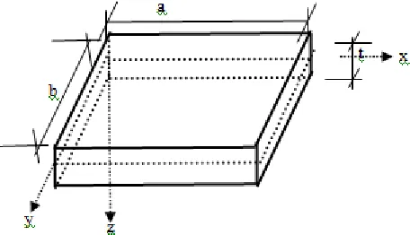
Fig. 1 shows an elastic isotropic and homogeneous thin rectangular plate of uniform thickness, t with arbitrary edge constraints. The plate is assumed to be completely flat. The plate parameters are invariants in Young modulus, E and
mass density, ρ; and the governing differential equation of motion for free vibration is given by Leissa et al.[1] as
expressed in Eq. (1).
Fig. 1: Isotropic Rectangular Plate showing Coordinate Dimensions
+ 2 + − = 0 (1)
= ∗
12(1− ) (2)
By defining the weighting function as V(x, y), the weak-form variational statement is formulated using Eq. (1); and is given as expressed in Eq. (3):
0 = ( , ) + 2 + − (3)
Integration by parts was carried out on Eq. (3) to trade differentiation from deflection w to weighting function V. Thus:
= + − (4) .
.
Also
2 = 2 + 2 −2 (5)
. .
And
= + − (6)
. .
− .
=− (7) .
By substituting Eqs. (4) through (7) into Eq. (3), the expression for energy functional and the natural boundary conditions is obtained as given by Eq. (8).
0 = + 2 + −
+ −2∂V
∂x ∂ w ∂x∂ ∂y+ V
∂ w ∂x∂y −
∂V ∂y
∂ w ∂y dx
+ V∂ w
∂x − ∂V ∂x
∂ w ∂x + 2V
∂ w
∂x∂y dy (8)
(4)
0 = + 2 + − dxdy (9)
Where V is weighting function; M is the mass density of the plate materials.
= ∗ (10)
= 1 (11)
Let Eq. (9) be transformed in the form as shown in Eq. (12):
+ 2 + = (12)
Then by substituting appropriate displacement function and weighting function into the left hand side (L.H.S.) of Eq. (12) and integrating appropriately yields the stiffness matrix. Similarly, by substituting the same displacement function and weighting function into the right hand side (R.H.S.) of Eq. (12) and integrating, yields the mass matrix.
Development of Algebraic Polynomial Displacement Functions
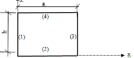
Fig. 2 shows a rectangular plate which can be idealized as a system consisting of series of orthogonal beam network. The deflection configuration of the plate can be approximated by a series of orthogonal beam deflection configurations. It is assumed that each beam element running along any coordinate direction is a good representative of other series of beams that run along the same direction.
Fig. 2: A Rectangular Plate with Arbitrary Edge Constraints, showing Coordinate Dimensions a and b
The constraint at each edge can be clamped, or simply supported or free; and a minimum of two boundary conditions must be satisfied on each edge.
Thus, for clamped edge condition, the boundary conditions to be satisfied are:
(∙,∙) = (∙,∙) = 0 (13)
For simply supported edge condition, the boundary conditions to be satisfied are:
(∙,∙) = (∙,∙) = 0 (14)
a
(∙,∙) = (∙,∙) = (∙,∙) = 0 (15)
Where (∙,∙) is the deflection; ′(∙,∙), ′′(∙,∙) and ′′′(∙,∙) are first, second and third partial derivatives with respect to coordinate axis respectively.
Then let the five-term static polynomial deflection configurations in x- and y-directions be defined as expressed in Eqs. (16) and (17) respectively:
( ) = (16)
( ) = (17)
Where and are undetermined coefficients.
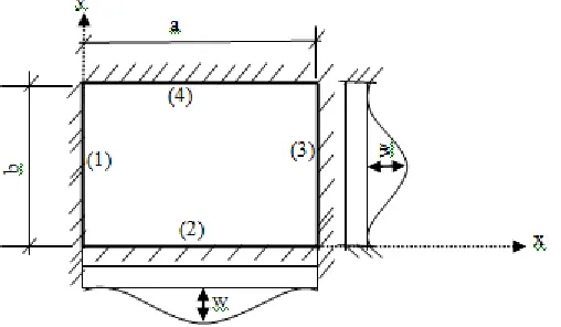
For demonstration, suppose Fig. 2 is a rectangular plate with all its edges clamped as replicated in Fig. 3
Fig. 3: A Rectangular Plate with all Eges Clamped; showing Orthogonal Beam Network Deflection Configurations.
By applying boundary conditions of Eq. (13) on Edges (1) and (3) at = 0 and = respectively, Eq. (16) yields an expression as expressed in Eq. (18):
( ) = ∗ −2 + (18)
To take care of series of beams running in the same direction, Eq. (18) is transformed as expressed in Eq. (19).
( ) = ∗ −2 + (19)
Similarly, by applying boundary conditions of Eq. (16) on Edges (2) and (4) at = 0 and = respectively, Eq. (17) yields an expression as expressed in Eq. (20).
( ) = ∗ −2 + (20)
To take care of series of beams running in the same direction, Eq. (20) is transformed as expressed in Eq. (21).
( ) = ∗ −2 + (21)
For n = 1, 2, 3, …
Thus, the algebraic orthogonal polynomial displacement functions for all clamped edges (CCCC) rectangular plate based on static deflection configuration are as expressed in Eq. (22).
( , ) = −2 + −2 + (22)
Where Amn is the amplitude of deflection, defined as expressed in Eq. (23).
= ( ∗ )∗( ∗ ) (23)
Thus by using the same procedure, the algebraic orthogonal polynomial displacement functions for any set of rectangular plate boundary conditions can be developed; and they are as shown in Table 1.
Table 1: Algebraic Orthogonal Polynomial Shape Functions for Rectangular Plate with various Boundary Conditions
Boundary
Conditions Algebraic Orthogonal Polynomial Shape Functions, w(x,y) CCCC
−2 + −2 +
SSSS
−2 + −2 +
CSCS
−2 + −2 +
CSSS 3
2 −
5
2 + −2 +
CCSS 3
2 −
5
2 +
3
2 −
5
2 +
CSFS
6 −4 + −2 +
CCCS
−2 + 3
2 −
5
2 +
CCCF
−2 + 6 −4 +
SSSF
−2 + 8 −4 +
CCSF 3
2 −
5
IV. NUMERICAL SOLUTION AND DISCUSSION OF RESULTS
Determination of Natural Frequencies
The plate parameters adopted in this work are:
= 10.92∗10 ; = 100 ; = 0.3; = 1.0 ; = 0.01 ; = ; =
With reference to Fig. 3 and Eq. (22), the algebraic orthogonal polynomial shape functions for all edges clamped rectangular plate are as expressed in Eq. (24).
( , ) = −2 + −2 + (24)
Where , = 1,2,3,⋯ Amn = amplitude of deflection. For small deflection theory, the parameter Amn will cancel out in Eq. (12) of the energy equation; and as such there is no loss in accuracy if Amn is taken to be unity. The values of m and n in Eq. (24) identify and define the modes for any given displacement function as shown in Eqs. (25) through (28). (1,1) = −2 + −2 + (25)
(1,2) = −2 + −2 + (26)
(2,1) = −2 + −2 + (27)
(2,2) = −2 + −2 + (28)
Where (1,1) is the first mode, (1,2) is the second mode, (2,1) is the third mode and (2,2) is the fourth mode. To calculate multiple natural frequencies of a system, the effect of modal interaction must be taken into account. In this work, the participations of the functions V and w in the energy equation of Eq. (12) were taken to represent the modal interaction at any given modal point. Equally, from small deflection theory, there exists symmetry in the stiffness distribution so that = . Therefore to determine the stiffness , let = = (1,1); to determine = , let = (1,2)and let = (1,1); to determine = , let = (2,1) and let = (1,1); to determine = , let = (2,2) and let = (1,1) and so on. In this work, all the complex computations were carried with the aid of Mathematica® commercial software. Thus (1,1) + 2 (1,1) + (1,1) = (29)
(2,1) (1,1)
+ 2 (2,1) (1,1)+ (2,1) (1,1) = = (31)
⋮
(2,2)
+ 2 (2,2) + (2,2) = (32)
The resulting stiffness matrix is given as expressed in Eq. (33).
[ ] = (33)
Using the plate parameters as adopted in this work for CCCC plate, then Eq. (33) in numerical values is expressed as in Eq. (34):
[ ] =
⎣ ⎢ ⎢ ⎢ ⎢ ⎢
⎡3.26531 1.63265 1.63265 0.81633
1.63265 1.1324 0.81633 0.56621
1.63265 0.81633 1.13241 0.56621
0.81633 0.56621 0.56621 0.37747⎦ ⎥ ⎥ ⎥ ⎥ ⎥ ⎤
10 (34)
The same procedure that was used for developing the stiffness matrix was also applied to the right hand side of Eq. (12) to develop the mass matrix.
Thus
(1,1) = (35)
(1,2)∗ (1,1) = = (36)
(2,1)∗ (1,1) = = (37)
⋮
The resulting mass matrix is as expressed in Eq. (39):
[ ] = (39)
Also using the plate parameters as defined, the numerical values of Eq. (39) with respect to CCCC plate is as expressed in Eq. (40):
[ ] =
⎣ ⎢ ⎢ ⎢ ⎢ ⎢
⎡2.51953 1.25976 1.25976 0.62988
1.25976 0.68714 0.62988 0.34357
1.25976 0.62988 0.68714 0.34357
0.62988 0.34357 0.34357 0.18740⎦ ⎥ ⎥ ⎥ ⎥ ⎥ ⎤
10 (40)
Suppose the difference between [ ] and [ ] is [ ], then
[ ] = [ ]−[ ] (41)
The determinant of [ ] is thus:
[ ] = ([ ]−[ ]) (42)
For nontrivial solution, Eq. (42) is set equal to zero. That is
([ ]−[ ]) = 0 (43)
Eq. (43) can be numerically simplified by pre-multiplying Eq. (43) by the inverse of Eq. (40) as shown in Eq. (44).
([ ] [ ]−[ ] [ ]) = 0 (44)
The result of the manipulation of Eq. (44) gives an expression as shown in Eq. (45).
⎣ ⎢ ⎢ ⎢ ⎢ ⎢
⎡1296.79− −2109.99 −2110.44 514.06
−1.61178 5514.9− −3.0878 −3140.29
−1.61178 −5.0098 5517.0− −3140.29
3.2754 9.8258 5.9816 11800.9− ⎦ ⎥ ⎥ ⎥ ⎥ ⎥ ⎤
= 0 (45)
clamped-clamped-functional formulated using weak-form variational principle; and Table 2 presents the results of the investigation along side with the results from previous works found in literature.
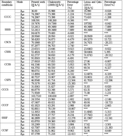
Table 2: First Four lowest Natural Frequencies of Rectangular Plate with various Boundary Conditions, at = 1
The triple star symbol, *** indicates that there is no result with respect 4th lowest natural frequency. Boundary
conditions
Mode Present work
[ / ]
Chakraverty (2009) [ / ]
Percentage Error
[%]
Leissa and Qatu (2011)
[ / ]
Percentage Error [%]
CCCC
36.00 35.988 -0.330 35.990 -0.028 74.2967 73.398 -1.224 73.410 -1.208 74.2967 73.398 -1.224 73.410 -1.208
108.591 108.260 -0.306 *** ***
SSSS
19.7476 19.7390 -0.044 197392 -0.043 53.2413 49.3480 -7.889 49.3480 -7.889 53.2413 49.3480 -7.889 49.3480 -7.889
84.6470 79.400 -6.608 *** ***
CSCS
28.9560 28.950 -0.021 28.9509 -0.018 58.4283 54.873 -6.479 69.3270 15.721 70.1868 69.327 -1.240 54.7431 -28.211
97.2977 94.703 -2.740 *** ***
CSSS
23.6515 23.646 -0.023 23.6463 -0.022 55.4824 51.813 -7.082 58.6464 5.395 62.2737 58.650 -6.179 51.6743 -20.512
91.8503 86.252 -6.491 *** ***
CCSS
27.0618 27.055 -0.025 27.06 -0.007 64.1546 60.550 -5.953 60.79 -5.535 64.3702 60.550 -5.953 60.54 -6.327
98.6751 92.914 -6.200 *** ***
CSFS
13.4904 12.687 -6.332 12.6874 -6.329 40.7537 33.067 -23.246 33.0651 -23.253 46.9548 41.714 -12.564 41.7019 -12.596
79.3170 63.260 -25.383 *** ***
CCCS
31.8363 31.827 -0.029 31.83 -0.020 66.8770 63.348 -5.571 63.35 -5.567 71.9549 71.083 -1.227 71.08 -1.231 103.7510 100.830 -2.897 *** ***
CCCF
24.5354 23.960 -2.402 24.02 -2.146 47.5407 40.021 -18.789 40.04 -18.733 65.1823 63.291 -2.988 63.49 -2.665
92.8811 78.139 -18.867 *** ***
SSSF
12.3053 11.684 -5.318 11.6845 -5.313 30.0426 27.757 -8.234 27.7563 -8.237 46.2809 41.220 -12.278 41.1967 -12.341
65.8793 59.360 -10.983 *** ***
CCSF
18.2369 17.555 -3.884 17.62 -3.501 43.7587 36.036 -21.431 36.05 -21.383 56.5625 51.862 -9.063 52.06 -8.649
Furthermore in this study, the variation of fundamental frequencies with aspect ratios (Beta) was investigated, and the results of the investigation were graphically presented as shown in Figure 4.
Fig. 4 Variation of Fundamental Frequencies with Aspect Ratios
Statistical Evaluation
In order to properly compare the present study’s results with the results from previous works found in literature, statistical analysis was carried out. The mean absolute percentage error values had to be evaluated. Also, the coefficient of determination and the correlation coefficient had to be evaluated as measures to determine the variation of the present study’s results with the results from previous works found in literature. Thus:
̅% =|∑ (
∗− )|
% (44)
∗=∑ ∗
(45)
=∑ ( −
∗)
∑ ( ∗− ∗) (46)
0.25 0.5 0.75 1 1.25 1.5
14
84
154
224
294
364
Beta
F
u
n
d
.
F
r
e
q
.(
w
1
1
)
CCCC
SSSS
0.25 0.5 0.75 1 1.25 1.5
8
78
148
218
Beta
F
u
n
d
.
F
r
e
q
.(
w
1
1
)
CCCS
CSFS
0.25 0.5 0.75 1 1.25 1.5
10
80
150
220
Beta
F
u
n
d
.
F
r
e
q
.(
w
1
1
)
CCSS
CCCF
0.25 0.5 0.75 1 1.25 1.5
10
80
150
Beta
F
u
n
d
.
F
r
e
q
.(
w
1
1
)
CSSS
CCSF
Where ̅ is the mean of the error; is the natural frequency of the present work at mode i; ∗is the corresponding natural frequency of the previous work found in literature at mode i; ∗ is the mean of the natural frequencies of the previous work found in literature; r is the correlation coefficient; and r2 is the coefficient of determination. The values in Table 2 were used to calculate the required parameters of Eqs. (44), (45) and (46) respectively.
Discussion of Results
From Table 2, it was discovered that the present study’s results with respect to fundamental frequencies are excellently stable when compared with the results from previous works found in literature for all the boundary conditions investigated. Also, the present work’s results were found to be on upper bounds. From statistical evaluation on the aggregation of natural frequencies computed for all boundary conditions, it was observed that 82.5% of them give good convergence to the results from previous works found in literature. Also from Table 2, and with reference to column 5, the mean absolute error between the present work’s results and the results from previous work found in [6] is 7.188%; and the coefficient of determination and correlation coefficient evaluated using the previous results found in [6] as standard were 0.99998 and 99.999% respectively. This implies that 99.998% of the variation between the present study’s results and those of the previous work done by [6] has been explained. Also with reference to column 7, the mean absolute error between the present study’s results and the results from previous work found in [1] is 6.325%. Similarly, the coefficient of determination and correlation coefficient evaluated using the previous results done by [1] as standard were 0.99996 and 99.998% respectively, which implies that 99.996% of the variation between the present study’s results and those of the previous work done by [1] has been explained. From the statistical analysis carried out, the present work’s results are acceptable for any engineering precisions. Furthermore, from Fig. 4, the variation of fundamental frequencies with plate aspect ratios exhibited soft-spring type. This indicates that at very low plate aspect ratio, the fundamental natural frequencies approach equivalent beam fundamental natural frequencies.
V. CONCLUSION
This paper applies weak-form variational principle and algebraic orthogonal polynomial displacement functions to determine the natural frequencies of rectangular isotropic plate with various boundary conditions. The natural frequencies computed herein in this work, in view of statistical interpretation, are in good agreement with results from previous works found in literature. Therefore, it is here-under concluded that weak-form variational principle has high competitive capability with other approximation techniques in dealing with problems of dynamic analysis of thin rectangular isotropic plates. Furthermore, it is here concluded that the application of algebraic polynomial displacement functions is capable and stable in yielding satisfactory approximations to any set of boundary conditions of rectangular plates.
REFERENCES
[1] Leissa, A. W. and Qatu, M. S., Vibrations of Continuous Systems, McGraw-Hill Company, New York, 2011.
[2] Singhal, P. and Bindal, G., “Generalized Differential Quadrature Method in the Study of Free Vibration Analysis of Monoclinic Rectangular Plates,” American Journal of Computational and Applied Mathematics, vol. 2, No. 4, pp 166-173, 2012.
[3] Reddy, J. N., Energy Principles and Variational Methods in Applied Mechanics, New York, John Wiley and Sons, 2002.
[4] Leissa, A. W., “Recent Research in Plate Vibrations 1981 – 1985 Part I: Classical Theory,” Shock and Vibration Digest, 19(2), pp 11-18, 1987. [5] Leissa, A. W., “Recent Research in Plate Vibrations 1981 – 1985 Part II: Complicating Effects,” Shock & Vibration, 19(3), pp 10 -24, 1987.
[6] Chakraverty, S., Vibration of Plates, CRC Press, Taylor & Francis Group, New York, 2009.
[7] Patil, A. S., “Free Vibration Analysis of Thin Isotropic Rectangular,” International Journal of Innovative Research in Science, Engineering and Technology, vol. 3, issue 4, pp 77 – 80, 2014.
[8] Yadav, D. P. S., Sharma, A. K. and Shivhare, V., “Effect of Stiffeners’ Position on Vibration Analysis of Plates,” International Journal of Advanced Science and Technology, vol. 80, No. 3, pp 31 – 40, 2015.
[9] Hatiegan, L. (Barboni), Hatiegan, C., Gillich, G. R., Hamat, C. O., Vasile, O. and Stroia, M. D., “Natural Frequencies of Thin Rectangular Plates Clamped on Contour Using the Finite Element Method,” Proc. of IOP Conference Series: Materials Science and Engineering 294 012033, pp 1-16, 2018.
[11] Kirişik, R. and Yüksel, Ş., “Free Vibration Analysis of a Rectangular Plate with Kelvin Type Boundary Conditions,” Shock and Vibration, 14, pp 447 – 457, 2007.
[12] Shu, C., Wu, W. X. and Wang, C. M., “Least Squares Finite Difference Method for Vibration Analysis of Plates,” (in Analysis and Design of Plated Structures, vol. 2 – Dynamics), Edited by Shnmugam, N. E. and Wang, C. M, CRC Press, USA, pp118 – 144, , 2007.
[13] Phamova, L. and Vampola, T., “Vibration Modes of a Single Plate with General Boundary Conditions,” Applied and Computational Mechanics, 10, pp 49-56, June 2016.
[14] Njoku, K. O., Ezeh, J. C., Ibearugbulum, O. M., Ettu, L. O. and Anyaogu, L., “Free Vibration Analysis of Thin Rectangular Isotropic CCCC Plate Using Taylor Series Formulated Shape Function in Galerkin’s Method,” Academic Research International, vol. 4, No. 4, pp 126 – 132, 2013.
[15] Ezeh, J. C., Ibearugbulem, O. M. and Ebirim, S. I., “Fundamental Natural Frequency for Isotropic Rectangular Plate Simply Supported on Three Edges with One Edge Free of Support (SSSF Plate),” Impact: International Journal of Research in Engineering & Technology (IMPACT: IJRET) vol. 2 Issue 2, pp 67 – 74, 2014.