Analysis of Petri Nets using Linear
Programming Techniques
V. Padma
1, Dr. K. Bhuvaneswari
2Research Scholar, Mother Teresa Womens University, Kodaikanal, India 1
Head, Department of mathematics, Mother Teresa Womens University, Kodaikanal, India 2
ABSTRACT: The Algebraic representation of polyhedral sets is an alternative tool for the analysis of structural and local properties of Petri nets. Some aspects of the issues of reachability, boundedness of a net are analysed and characterized by the means of linear system of inequalities. In most cases, the structural analysis techniques such as linear programming based technique instead of integer programming can be used to check these properties therefore enabling the validation of very large nets.
I. INTRODUCTION
Petri nets have become a widely used tool for modelling and analyzing large , complex and discrete event systems. They appear in computer science as well as in Operations Research for modelling a quite large number of problems such as information processing, communication network design, scheduling and controlling of manufacturing processes. Here we focus on some aspects of the analysis of petri nets.An important issue is for example to know whether it is able to realize and complete all the tasks for which it has been designed .Among the related properties which are commonly analysed are the boundedness and the liveness of the net in order to certify that neither traps nor deadlock may occur. These two properties are linked to the issue of reachability which in turn one of the key concept of system theory. In that sense it is quite natural to view the evolution of the marking on the places of the graph as a linear time invariant discrete system. If Mk is the vector of marks on the space of places of the net at time k,𝜎k is a control vector of firings on the space transitions and C is the incidence matrix of the graph, then the dynamic state equation is Mk+1 = Mk + C σk Infact linear system theory is of limited help when dealing with Petri nets. Some partial characterization of controllability and reachability are given in Murata but these results are not sufficient and cannot be exploited practically . On the other hand linear algebra and in particular some duality results for systems of linear inequalities gave rise to a few interesting propositions about boundedness , liveness and concurrency [2].This approach constitutes a valid alternative,to the classical analysis where we must build a reachability tree (i.e)the tree of all feasible firing sequences from a given initial state. However the computational complexity is very high to test the conditions on the set of integers Peterson[2] has mentioned the possibility to relax the integrality condition and to use linear programming for the detection of semiflows in the net. We now extend this statement ,to some Petri nets using its languages,proving its validity for the conditions of boundedness,liveness and for reduction techniques.Duality is then used to yield some insights on the geometry of the reachable set.
This paper is organized as below.Section 2 presents basic definitions . Section 3 investigates the examples for the analysis of Petri nets using Linear Programming Techniques. Section 4 concludes this paper with the extension of future work on identifying Place/transition nets.
II. PRELIMINARIES
In this section we will quickly review the Petri net formalism used in the paper, referring to [1] for a comprehensive introduction to petri nets.
2.1. Background on petri nets
Pre : P × T → ℕ and Post : P × T → ℕ are the pre - and post – incidence functions that specify the arcs; C =Post – Pre is the incidence matrix.
A marking is a vector M : P → ℕ that assigns to each place of a P/T net a nonnegative integer number of tokens represented by black dots. We denote M (p) the marking of place p.
A P/T system or net system N, M₀ is a net N with an initial marking M0 .
A transition t is enabled at M iff M ≥ Pre (∙ , t ) and may fire yielding the marking M′ = M + C (∙ ,t ) = M + C ∙ σ where 𝑡 ∈ℕn is a vector whose components are all equal to 0 except the component associated to transition t that is equal to 1.We write M [ 𝜎 to denote that the sequence of transitions σ is enabled at M, and we write M [ 𝜎 M′to denote that the firing of σ yields M′.
A marking M is reachable in N, M0 iff there exists a firing sequence σ such that M0 [ 𝜎 𝑀.In such a case the state equation M = M0 + C ∙ 𝜎 holds ,where 𝜎 ϵ ℕn is the firing vector of σ , i.e., the vector whose 𝑖𝑡ℎ entry represents the number of times the transition ti is contained in σ. The set of all markings reachable from M0 defines the reachability set of N,M₀ and is denoted by R(N,M0).
2.2. Petri net Languages
Given a Petri net system N, M₀ we define its free- language as the set of its firing sequences L (N,M0) = σ ϵ ∈ T∗, M₀[ σ .
We also define the set of firing sequences of length less than or equal to 𝑘 ∈ ℕ as: Lk ( N,M0 ) = σ ∈ L N, M₀ σ ≤ 𝑘 . Finally given a language ℒ ⊂ T *and a vector 𝑦 ∈ ℕ𝑛we denote
ℒ(𝑦) = σ ∈ ℒ σ = 𝑦 the set of all sequences in ℒ whose firing vector is 𝑦.
2.3. Special constraint sets (CS)
We define a special class of linear constraint sets (CS)
Definition 2.3.1: Given A∈ ℝm ×n and b ∈ ℝm , consider the linear constraint set :
∁ 𝐴, 𝑏 = 𝑥 ∈ ℝⁿ 𝐴𝑥 ≥ 𝑏
The set ∁ (𝐴 , 𝑏) is called :
ideal: if 𝑥 ∈∁ (𝐴 , 𝑏) implies 𝛼𝑥 ∈ ∁ 𝐴, 𝑏 𝑓𝑜𝑟 𝑎𝑙𝑙 𝛼 ≥ 1;
rational: If A ∈ℚ𝑚 ×𝑛 and b∈ ℚ𝑚,i.e., if the entries of matrix A and of vector b are rational.
Definition 2.3.2: A Petri net N is said to be (partially) consistent if there exists an n-vector 𝑥 of positive (non negative) integers such that C 𝑥 = 0,𝑥 ≠ 0.
Proposition 1: If a CS is ideal and rational , then it has a feasible solution if and only if it has a feasible integer solution.[4]
Proof: The if part is trivial.
To prove the only if part , we reason as follows. If there exists a solution there exists a basis solution 𝑥𝐵 , i.e such that 𝑥𝐵 = A−1𝐵 𝑏, where A𝐵 is obtained by A selecting a set of basis columns.
If the CS is rational the entries of A𝐵 and b are rational ,hence the entries of A−1B and of 𝑥𝐵 are rational as well.
If the CS is ideal, we just need to multiply the rational vector 𝑥𝐵by a suitable positive integer to obtain an integer solution.
Definition 2.3.3: Let ℒ ⊂ 𝑇*
be a finite prefix - closed language and let k∈ ℕ then we define the set of enabling conditions
ℰ = 𝑦, 𝑡 ∂σ ∈ ℒ ∶ σ < 𝑘 , σ ∈ ℒ 𝑦 , σ 𝑡 ∈ ℒ) (1)
⊂ ℕⁿ × 𝑇
and the set of disabling conditions
𝒟 = 𝑦, 𝑡 ∂σ ∈ ℒ ∶ σ < 𝑘 , σ ∈ ℒ 𝑦 , σ𝑡 ∉ ℒ) (2)
⊂ ℕⁿ × 𝑇
Theorem 1: The reachability problem for type ℒ PN is a NP- complete.
III.ANALYSIS OF PETRI NETS
Example 1:
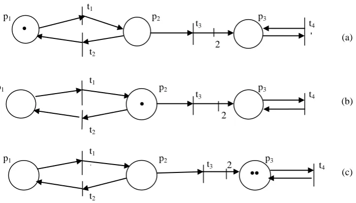
Let us consider the net system N, M₀ in Fig 1(a).If transition t1 fires the net reaches the networking in Fig 1(b) because one token is removed from p1 to p2 . Now both transitions t2 and t3 are enabled. If t3 fires the net reaches the new marking in Fig 1(c),because one token is removed from p2 and two tokens are added to p3 , being „2‟ the weight of the arc going from t3 to p3.
Next, the only enabled transition is t4 ,but its firing doesnot change the marking being C (p3 ,t4) =0 .
Fig. 1. Place /Transition net systems
REACHABILITY TREE:
A marking M is reachable in N, M₀ if there exists a firing sequence σ such that M [ σ M. The reachability set of
N, M₀ ,denoted as R(N,M) is the set of markings that are reachable from M (i.e)
R (N,M) = 𝑀 ∈ ℕⁿ ∂σ ∈ T∗∶ M₀[ σ M .
The reachability set may never be an empty set because it always includes atleast the initiai making .Moreover ,it may either be finite or infinite. In the case of the P/T net system in Fig 1(a) the reachability set is
R (N,M) = 1,0,0 ᵀ , 0,1,0 ᵀ 0,0,2 ᵀ .
The reachability graph is
If the rechability set is infinite ,then obviously the reachability graph is infinite as well . In this example the coverability graph is finite and it provides the necessary (not sufficient ) for determining if a marking is reachable (or) if a sequence is firable.
p1
p1
p1
p2
p2
p2
p3
p3
p3 t1
t1
t1 t2
t2
t2
t3
t3
t3
t4
t4
t4 2
2
2
(a)
(b)
(c)
t1
t2 t3 t4
STATE EQUATION (MATRIX ANALYSIS)
A linear algebraic equation can be written to describe the evolution of the net system after the firing of a sequence σ∈
T* . Let us consider a net system N, M₀ with incidence matrix C. if M is reachable from M0 firing σ ,then
M = M₀ + C ∙ σ (3) Consider a net system with a firing sequence σ = t1t2 t1t2t1t3. The firing vector associated to σ is σ = [3 2 1 0]T and we can easily verify that the marking M = [0 0 2]T obtained from firing σ satisfies equation (3) where C = Post –Pre : P × T → ℤ .
A net N = P, T, Pre, Post with a set of places P = { p₁ ,p₂ ,p₃ } and the set of transitions T = {t₁ ,t₂ ,t₃ ,t₄ ]. Here,
Pre =
1 0 0 0 1 1 0 0 0
0 0 1
Post =
0 1 0 1 0 0 0 0 2
0 0 1
C =
−1 1 0 1 −1 −1
0 0 2
0 0 0
A transition is enabled at marking if M ≥ Pre ( . ,t )
M = 1 0 0
+
−1 1 0
1 −1 −1
0 0 2
0 0 0 3 2 1 0 = 0 0 2
LINEAR PROGRAMMING TECHNIQUE
The possibility offered by Petri nets to describe the state space of a discrete event system that may have absolutely no algebraic structure, with a set of integers vectors has an important implication .One of the main advantages of Petri nets is that the state is a vector of non-negative integers ,which leads to the structural analysis of the Petri net system in Linear Programming Technique.In this technique the enabling condition can be expressed using linear inequalities , while the effect of firing a transition can be expressed as linear assignments.
Theorem 2: For a strongly connected live marked graph G, M₀ ,we have
max Mᵀ W M ∈ R M0 = min M0ᵀ I I ≥ W , CᵀI = 0 (4)
min Mᵀ W M ∈ R M₀ = max M₀ᵀ I I ≤ W , CᵀI = 0 (5)
Proof : Since M₀ is live, M ∈ R (M₀) iff M =M₀ + C∙ X where X is an n×1 vector of non negative integers. Thus ,the left –hand side of (4) can be written as the following linear programming problem:
Max U = Aᵀ z subject to Dz ≤ M₀ and z ≥ 0 (6)
Where A = W
0 z = M
X D = Im − C ,and is Im the identity matrix of order m. The dual problem of
(6) can be stated as
min V = M0T Y subject to DT Y ≥ C (7) Y = I is unrestricted, DT Y ≥ C is equivalent to I ≥ W ( W is an m×1 column vector whose ith entry is W (ei) a non negative integer weight of arc ei ) and CT I ≤ 0. However CT I ≤ 0 is equivalent CT I = 0 since the sum of the „n‟ rows in CT is always zero ,
(i.e) ., 1 1 … … … 1 AI = 0 I = 0 . It is well known in linear programming that the optimal solution of (6)or (7) is an extreme point of the corresponding constraint set. Therefore the optimal values of (6) and (7)are attained at integral values and (4) follows from the theory of duality.Solving (6) we found out the solution as integers and also in this example the reachability ,boundedness and liveness of the petri net is preserved.
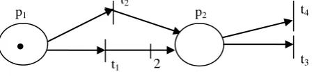
Example 2 : Let us consider a net system in Fig (2).
Fig. 2. Petri net system in example 2
p1 p2
REACHABILITY TREE
In this example the reachability set is given based on the transition it fired.
R(N,M₀ ) = 1,0 ᵀ , 0,2 ᵀ , 0,1 ᵀ , 0,0 ᵀ if it follows the firing sequence t₁ t₃ t₃ . R(N,M₀ ) = 1,0 ᵀ, (0,1)ᵀ if it follows the firing sequence t₂ t₃ and t₂t₄.
R(N,M₀ ) = 1,0 ᵀ, 0,2 ᵀ, (0,1)ᵀ which follows the firing sequence t₁t₄. The reachability graph is
The coverability graph is finite for each firing sequences and it provides the necessary condition for determining if a marking is reachable or if a sequence is firable.
STATE EQUATION: (Matrix Analysis)
If M is reachable from M₀ firing „σ‟ then
M = M₀ +C ∙ σ (8)
For the given Petri net we have to fix the firing sequence and analyse its state equation.In the example consider a net system with a firing sequence σ = t₁t₃t₃ .The firing vector associated with the firing sequence is σ = [1 0 2 0]ᵀ and we can easily verify that the marking M = [0,1]ᵀ . P = { p₁ ,p₂ }, T = { t₁ ,t₂ ,t₃ ,t₄ },
Pre = 1 1 0 0 0 1
0
1 , Post =
0 0 0 2 1 0
0
0 , C =
−1 −1 0 2 1 −1
0
−1 , M₀ = 10
∴ M = 1 0 +
−1 −1 0 2 1 −1
0 −1
1 0 2 0
In a Petri net a sequence of transition is a string and a set of strings is a language. The set of all possible sequences of actions characterizes the system.These sequences of transitions can be of extreme importance in using Petri nets.Assume that a new system has been designed to replace an existing one.The behaviour of the new system is to be identical to the old system.If both the system are modeled as petri nets, then the behaviours of these nets should be identical,and so their languages are equal.The Petri net language provides formal basis for stating the equivalence of two systems.
A particular instance in which equivalence is important is optimization.Optimizing a petri net involves creating a new Petri net which is equivalent (languages are equal) but for which the new net is “better” than the old one.Thus one optimization problem might be to reduce P + T without changing the behaviour of the net . For purposes of optimization ,a set of language preserving transformations might be useful of a transformation applied to a petri net produces a new Petri net with a same language, then it is language preserving . petri net languages can also be useful for analysis of Petri nets. Here we have considered a class of Petri nets (called Type ℒ ) for which the reachability sets can be characterized by Linear Programming Problem. In this case we can solve the problem in two criteria optimization problem that first requires identifying a net with the minimal number of places allows one to optimize and the second one is the number of arcs or of tokens in the initial marking.We consider here the global priorities [5] the objective function for the Linear Programming Problem as in [4]
Min f M₀ ,Pre,Post ) = 1T ∙ M
0+1T∙ Pre ∙ 1 + 1T Post ∙ 1 subject to 𝒩(ℰ, 𝓓)
Where
[1 0] [0 2]
[0 2]
[0 1] [0 0]
[0 1] [0 0]
[0 1] [0 0]
[0 0]
t1 t4 t4
t4 t2 t1
t3
𝒩(ℰ, 𝒟) ≜
M₀ + 𝑃𝑜𝑠𝑡 ∙ 𝑦 — 𝑃𝑟𝑒 ∙ ( 𝑦 + 𝑡 )≥ 0 , ∀ (𝑦, 𝑡) ∈ ℰ
M₀ ( p(𝑦,𝑡))+ 𝑃𝑜𝑠𝑡 (p(y,t), ∙ ) ∙𝑦 − 𝑃𝑟𝑒 p y,t , ∙ ∙ 𝑦 + 𝑡 ≤ −1 , ∀ 𝑦, 𝑡 ∈ 𝒟
CS(1) M₀ ∈ ℝ≥0𝑚
𝑃𝑟𝑒, 𝑃𝑜𝑠𝑡∈ℝ≥0𝑚 ×𝑛
Let us consider a language from example 2
ℒ = ε , t1 , t2 , t1t3 , t1 t4 , t2t3 , t2 t4 and let k = 2.
We have additional information : the transition t1 and t2 have only one input place and transition t3 and t4 are in a free choice relation .The set of enabling and disabling constraints are respectively:
ℰ = ε , t1 , ε , t2 , t1, t3 , t1, t4 , t2, t3 , t2, t4
𝒟 = ε , t3 , ε , t4 , t1, t1 , t2, t1 , t3, t1 , t4, t1 , t2, t2 , t3, t2 , t4, t2
A net system solution of 𝒩(ℰ, 𝒟) CS(1) computed by simplex method and the solution we found out was integers.Since the assumed petri net in example (2) is a small Petri net which can be solved by any commercial LP solver(LINGO).But in the case of large Petri nets the number of constraints and variables are more in number which leads to the complexity of preserving the system properties to be analysed.conversely ,techniques to transform an abstract model into a more refined model in a hierarchical manner can be used for synthesis.There exist many transformation techniques for Petri nets.One of the technique is to reduce one Petri net problem to another which preserves the properties of the original net.
IV. CONCLUSION
In this paper we investigate the property analysis of petri net and its language using Linear Programming Technique(LPT).Two simple examples are analysed with their properties and in general only necessary or sufficient conditions are obtained.The basic idea pointed out here is that the approach allows the study of many important qualitative and quantitative properties using well known polynomial complexity algorithms (rank computation ,Linear programming solution etc.,).As a possible line of future research , the extension of this procedure to analyse large Petri nets by transformation which preserves the properties to be studied.Reduction methods are a special class of transformation methods in which a net system S = 𝒩, M₀ is transformed into a net system S′ = 𝒩′, M0′ preserves the properties of the original net.The linear programming techniques can be applied to the reduced net.
REFERENCES
[1] T. Murata, “Petri nets: Properties ,analysis and applications”, in Proc. IEEE, vol. 77, no. 4, pp. 541580, 1989. [2] J.L. Peterson, “Petri Net Theory and the Modelling of Systems”, Englewood Cliffs, NJ, Prentice-Hall Inc., 1981.
[3] H. Yen, “Integer Linear Programming and the Analysis of Some Petri Net Problems”, Theory of computing systems (formerly, Mathematical Systems Theory), vol. 32, no. 4, pp. 467485, 1999 (Postscript).
[4] M.P. Cabasino, A. Giua, C. Saetzu, “Linear Programming Techniques for the Identification of Place/Transition Nets”, CDC08: 47th IEEE Conf.
on Decision and Cotrol (cancun, Mexico), pp. 514520, 2008.
[5] R.E. Burnard, F.Rendi, Lexicographic bottleneck problems, Operations Research Letters, vol. 10, pp. 303308, 1991.
[6] A. Giua and C. Seatzu, “Identification of free-labeled Petri nets via integer programming”, In Proc. 44th IEEE Conf. on Decision and Control,
Seville, Spain, 2005.
[7] M. Silva, Petri Nets, in Automation and Computer Engineering,Madrid, Spain, Editorial AC, (in Spanish) 1985.