Longitudinal Functional Data Analysis with Biomedical Applications.

ABSTRACT

PARK, SO YOUNG. Longitudinal Functional Data Analysis with Biomedical Applications. (Under the direction of Ana-Maria Staicu.)

Longitudinal functional data consist of functional observations, e.g. profiles or images,

collected from each of many subjects at multiple sequential instances (often visits). A major challenge in longitudinal functional data analysis is the presence of very complex dependence structure due to both within- and between-curves correlations, along with high dimensionality. This dissertation proposes novel statistical modeling and inference methods to address some fundamental scientific questions commonly arising from studies collecting longitudinal functional data, in a computationally efficient way.

the underlying process over time, allows prediction of full trajectories at unobserved visit times, and is computationally efficient. Theoretical properties of this framework are stud-ied and numerical investigations confirm excellent behavior in the finite sample setting. The proposed method is motivated by and applied to the Diffusion Tensor Imaging study of multiple sclerosis. Furthermore we provide interactive graphic tools inRto help explore longitudinal functional data and visualize the various model components and prediction obtained using the proposed method.

© Copyright 2017 by So Young Park

Longitudinal Functional Data Analysis with Biomedical Applications

by So Young Park

A dissertation submitted to the Graduate Faculty of North Carolina State University

in partial fulfillment of the requirements for the Degree of

Doctor of Philosophy

Statistics

Raleigh, North Carolina 2017

APPROVED BY:

Marie Davidian Soumendra Lahiri

Luo Xiao Ana-Maria Staicu

DEDICATION

BIOGRAPHY

ACKNOWLEDGEMENTS

I would like to take this moment to express my deepest gratitude to my advisor, Dr. Ana-Maria Staicu for her endless support and guidance throughout my graduate studies. Her passion to research and professionalism have truly motivated me to constantly improve my academic and personal life.

I would also like to extend my appreciation to my committee members, Drs. Marie Davidian, Soumendra Lahiri, and Luo Xiao, for sharing their time and insights into this research, and to Dr. Anne McLaughlin for serving as the graduate school representative. I would like to thank Dr. Luo Xiao for providing many professional opportunities as well as financial support. I am also very grateful for all of the faculty members, staffs, and fellow graduate students in Statistics department at North Carolina State University. In particular, I want to thank my dear friends, Marcela Alfaro Cordoba, Matthew Austin, Janet Kim, Cai Li, Md Nazmul Islam, Saebitna Oh for always being supportive and making my graduate school life fun and memorable.

TABLE OF CONTENTS

LIST OF TABLES . . . vii

LIST OF FIGURES . . . ix

Chapter 1 Introduction . . . 1

1.1 Overview . . . 1

1.2 Contributions and Outline . . . 5

1.3 Smoothing . . . 6

1.3.1 Smoothing using Penalized Basis Expansions . . . 7

1.4 Functional Principal Component Analysis . . . 9

Chapter 2 Simple Fixed Effects Inference for Complex Functional Models 12 2.1 Introduction . . . 12

2.2 Modeling framework . . . 15

2.3 Confidence bands forµ(s, x) . . . 20

2.4 Hypothesis testing for µ(s, x) . . . 25

2.5 Application to physical activity data . . . 27

2.6 Simulation Study . . . 32

Chapter 3 Longitudinal Functional Data Analysis . . . 38

3.1 Introduction . . . 38

3.2 Modeling longitudinal functional data . . . 41

3.3 Estimation of model components . . . 44

3.3.1 Step 1: Mean function . . . 44

3.3.2 Step 2: Marginal covariance. Data-based orthogonal basis . . . 45

3.3.3 Step 3: Covariance of the time-varying coefficients . . . 46

3.3.4 Step 4: Trajectories reconstruction . . . 48

3.4 Implementation using available softwares . . . 48

3.5 Theoretical properties . . . 49

3.5.1 Response curves measured without error . . . 50

3.5.2 Response curves measured with smooth error . . . 53

3.5.3 Extensions . . . 54

3.6 Simulation study . . . 55

3.7 DTI application . . . 57

3.8 Visualization using Interactive Graphics . . . 62

Chapter 4 Significance Testing in Longitudinal Functional Data . . . 66

4.1 Introduction . . . 66

4.3 Testing Procedure . . . 71

4.3.1 Implementation . . . 74

4.3.2 Pseudo Likelihood Ratio Test . . . 75

4.4 Simulation Study . . . 78

4.4.1 Data Generation . . . 78

4.4.2 Details on Estimation . . . 79

4.4.3 Competitive Methods . . . 80

4.4.4 Numerical Results . . . 81

4.5 Diffusion Tensor Imaging Study . . . 84

Chapter 5 Conclusion . . . 87

References . . . 90

Appendices . . . 104

Appendix A Additional Details for Chapter 2 . . . 105

A.1 Validating the BLSA Testing Results via Simulation Study . . . 105

A.2 Additional results for the performance of the confidence bands . . . 107

A.3 Results obtained by bootstrapping observations by subject . . . 109

A.4 Result for the case of nonparametric modeling . . . 113

A.5 Results for the case of having non-normal errors . . . 115

Appendix B Additional Details for Chapter 3 . . . 120

B.1 Proofs of theoretical results given in Section 3.5 . . . 120

B.1.1 Case when response curves are measured without error (Sec-tion 3.5.1) . . . 120

B.1.2 Case when response curves are measured with smooth error (Section 3.5.2) . . . 154

B.2 Additional details for the simulation experiment . . . 157

B.2.1 Description of the study . . . 157

B.2.2 Additional results . . . 160

B.3 Additional figures for the DTI data analysis . . . 163

B.4 Additional Figure for Interactive Graphics . . . 166

Appendix C Additional Details for Chapter 4 . . . 167

C.1 Additional Simulation Results . . . 167

LIST OF TABLES

Table 2.1 Simulation results using bootstrap of subject-level residuals and 95% nominal level; results are based on 500 MC samples. . . 36 Table 2.2 Empirical Type I error of the test statistic T based on theNsim = 1000

MC samples. . . 37 Table 3.1 Estimation and prediction accuracy results based on Nsim = 1000

sim-ulations . . . 58 Table 3.2 Comparison between the proposed method and Chen & M¨uller (2012)

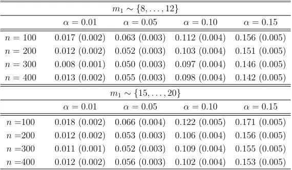
in the presence of correlated errors. Results based on Nsim = 1000 simulations . . . 59 Table 4.1 The empirical type I error rates of the proposed method (pLRT-MT)

based on 5000 simulations. Standard errors are presented in parentheses. 83 Table 4.2 Computation time (in seconds) based on 200 simulations when n = 200. 83 Table A.1 Empirical type I error of the test statistic T based on the Nsim = 1000

MC samples; Mean function is µ(s, x) = cos(2πs), τ = 0 . . . 106 Table A.2 Simulation results using bootstrap of subject-level residuals and 85%

nominal level; results are based on 500 MC samples. . . 107 Table A.3 Simulation results using bootstrap of subject-level residuals and 90%

nominal level; results are based on 500 MC samples. . . 108 Table A.4 Simulation results using bootstrap of subject-level observations and

85% nominal level; results are based on 500 MC samples. . . 110 Table A.5 Simulation results using bootstrap of subject-level observations and

90% nominal level; results are based on 500 MC samples. . . 111 Table A.6 Simulation results using bootstrap of subject-level observations and

95% nominal level; results are based on 500 MC samples. . . 112 Table A.7 Simulation results for the case of time-varying covariateXij using

boot-strap of subject-level observations; results are based on 500 MC samples.112 Table A.8 Simulation results fitting bivariate mean function using bootstrap of

subject-level residuals and 85% nominal level; results are based on 500 MC samples. . . 113 Table A.9 Simulation results fitting bivariate mean function using bootstrap of

subject-level residuals and 90% nominal level; results are based on 500 MC samples. . . 114 Table A.10 Simulation results fitting bivariate mean function using bootstrap of

Table A.11 Simulation results for the case of having non-Gaussian errors using bootstrap of subject-level residuals and 85% nominal level; results are based on 500 MC samples. . . 116 Table A.12 Simulation results for the case of having non-Gaussian errors using

bootstrap of subject-level residuals and 90% nominal level; results are based on 500 MC samples. . . 117 Table A.13 Simulation results for the case of having non-Gaussian errors using

bootstrap of subject-level residuals and 95% nominal level; results are based on 500 MC samples. . . 118 Table A.14 Empirical Type I error of the test statisticT based on theNsim = 1000

MC samples for the case of having non-Gaussian errors. . . 119 Table B.1 Simulation results for estimation and prediction accuracy based on

Nsim = 1000 simulations (white noise only) . . . 161 Table B.2 Computational time (seconds) corresponding to table 3.1 . . . 162 Table B.3 Computational time (seconds) corresponding to table B.1 . . . 162 Table C.1 The empirical type I error rates of the proposed method based on 5000

simulations. Standard errors are presented in parentheses. . . 168 Table C.2 The empirical type I error rates of the ZC-MT and Bootstrap-MT

meth-ods based on 5000 simulations. Standard errors are presented in paren-theses. . . 169 Table C.3 The empirical type I error rates of the proposed test and other

LIST OF FIGURES

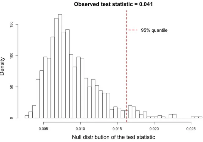
Figure 2.1 The null distribution of the test statistic in (2.4) for the null hypothesis that there is no effect of age on activity. The red dashed line is the 95 percent quantile of the null distribution of the test statistic. . . 29 Figure 2.2 Heat map of average of bootstrap estimates of log counts as a bivariate

function of time of day and age (left panel) and average of bootstrap estimates of log counts for five different age groups (right panel). . . 30 Figure 2.3 Heat maps of joint confidence bands for the estimate µ_b(t, Age) given

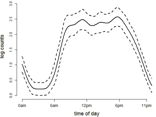
in the left panel of Figure 2.2. The legend on the right applies to both plots. . . 30 Figure 2.4 Average of bootstrap estimates of log counts as a function of time of

day at age 60 and the associated joint confidence bands. . . 31 Figure 2.5 Association of body mass index with mean log counts as a function of

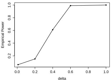
time of day and the associated joint confidence bands. . . 31 Figure 2.6 Estimated power curves for testing H0 : µ(s, x) = η(s) using level

of significance α = 0.05, when the true mean function µ(s, x) = 2 cos(2πs) + δ(x/4− s)3 _{for δ = 0.01,2,4,6. The results are based} on Nsim = 500 MC samples. . . 37 Figure 3.1 Left panel: 95% pointwise and joint confidence bands of the slope

function βt(s) of µ(s, t) using bootstrap; Right: final mean estimate, ˆ

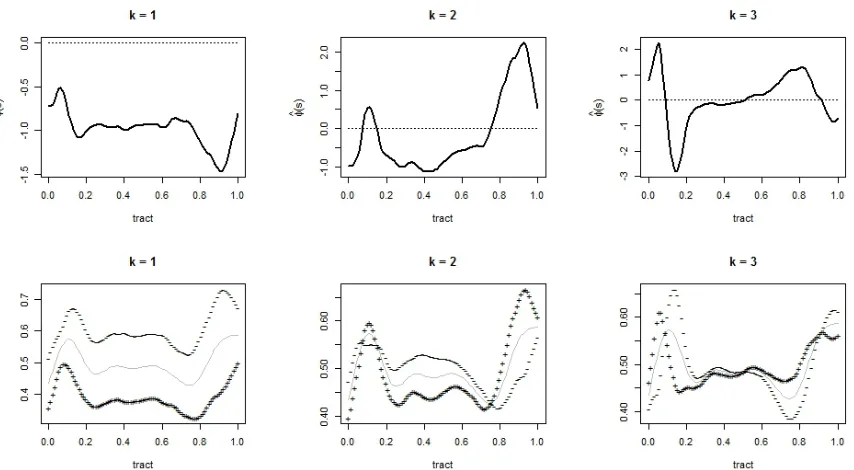
µ(s, t) = ˆµ0(s) . . . 60 Figure 3.2 Top: First three eigenfunctions of the estimated marginal covariance;

Bottom: estimated mean function µ_b0(s) (gray line) ± 2 q

b

λkφb_k(s) (+ and −signs, respectively) . . . 61 Figure 3.3 Estimated time-varying coefficients ξb_ik(t) fork = 1,2 and 3 using REM 62 Figure 3.4 Predicted values of FA for the last visits of three randomly selected

subjects; actual observations (gray); predictions using our model (black solid) and using the naive approach (black dashed) . . . 63 Figure 3.5 Screenshot showing tab 1 of the interactive graphic. The plots show

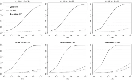
observed data of all subjects (top) and of the selected subject (bottom). 65 Figure 4.1 Estimated size and power curves for testing H0 :µ(s, t) =µ0(s) using

Figure A.1 Estimated power curves for testingH0 :µ(s, x) =η(s) usingα= 0.05, when the true mean function µ(s, x) = cos(2πs) +δ(µ_b(s, x)−cos(2πs)) for δ = 0.01,2,4,6,8. Results are based on Nsim = 500 MC samples. . 106 Figure A.2 Normal, skew-normal, and t distributions used to generate white noises.115 Figure B.1 Fitted varying coefficient model, µ_b(s, t) = _bµ0(s) +βb_t(s)t (left), and

estimated slope function, βb_t(s) (right) . . . 163 Figure B.2 Scree plot of the marginal FPCA . . . 163 Figure B.3 Estimated eigenfunctions of the marginal FPCA for FA with PVE = 95%164 Figure B.4 Estimated basis coefficient functions,ξb_ik(t) using a random coefficients

linear model . . . 165 Figure B.5 Screenshot showing tab 2 of the interactive graphic. The plots show the

third estimated eigenfunctionφb₃(s) (top) and the predicted trajectory of the selected subject at (scaled) visit time t= 0.3 (bottom) . . . 166 Figure C.1 The original DTI data (left) and one simulated data that mimic the

Chapter 1

Introduction

1.1

Overview

Functional Data Analysis (FDA) is an actively growing research area in Statistics that involves data with each observation being a function instead of a single value. For illus-tration consider marathon data, where elapsed time was recorded at every mile of the race for each of 105 male participants who completed the 2016 U.S. Olympic Team Trial Marathon. In this example, FDA views a set of elapsed times from each participant as a function of miles and treat it as a single datum. Enabled by rapid advancement of technology in recent years, such data have become commonly collected in many scientific applications across different disciplines. Intensive statistical researches have naturally fol-lowed to address challenges posed by functional data and have made great progress on both theoretical and methodological developments in FDA. For comprehensive reviews of FDA we direct the reader to monographs, Ramsay & Silverman (2005); Ferraty & Vieu (2006); Ramsay et al. (2009); and Horv´ath & Kokoszka (2012) among others.

where Yir is the rth repeated measurement for subject i corresponding to sir ∈ S for some compact interval S. In the marathon data example, Yir corresponds to the elapsed time recorded at mile sir for participant i. The key idea of FDA is to view the observed profile {Yir :r = 1, . . . , Ri} as a realization Xi(·) of a smooth unknown random process

X(·) that is observed at finite grid of points {sir :r = 1, . . . , Ri} and is corrupted with measurement errors {ir :r= 1, . . . , Rr}. That is, the observed data are modeled as

Yir =Xi(sir) +ir, (1.1)

whereXi(·)’s are independent and identically distributed (iid) square integrable random elements in L2(S) with unknown smooth mean and covariance functions, and measure-ment errors ir’s are iid with mean zero and variance σ2. FDA mainly considers two sampling designs: (i) dense design where the set of sampling points for each subject,

{sir : r = 1, . . . , Ri}, is dense in its domain S and (ii) sparse design where the number of repeated measures per subject, Ri, is relatively small and the set of sampling points for each subject, {sir : r = 1, . . . , Ri}, is random and irregular. In the sparse design setting, it is assumed that the set of pooled sampling points across all the subjects,

{sir :i= 1, . . . , nand r = 1, . . . , Ri}, is dense in its domain S.

the data. We detail the FPCA method in Section 1.4 for both dense and sparse design settings. Due to a variety of its uses FPCA has been served as a building block of many methodologies in FDA: functional linear regression (Cardot et al., 2003b; Yao et al., 2005b; Kim et al., 2015), conditional FPCA (Cardot, 2007), multilevel FPCA (Di et al., 2009), and FPCA-based optimal design (Park et al., 2016b) to name a few. In Chapter 3 we also borrow the idea of FPCA and develop a novel parsimonious modeling framework for longitudinal functional data.

While tremendous progress has been made in FDA, most of existing methodologies are developed for independent functional data, where only one curve is observed from each of the subjects, as described in (1.1). It is relatively recent that repeated functional data are considered in the literature, though an increasing number of studies now routinely collect such complex-correlated functional data. A major characteristic of these data is the presence of a strong between-curves correlation induced by multiple functions observed on the same observational unit, often subject.

been studied in Bosq (2000), Hyndman & Shang (2009), Horv´ath & Kokoszka (2012), Hormann & Kokoszka (2012).

In this dissertation we focus our study on longitudinal functional data, which consist of functional observations, e.g. profiles or images, collected from each of many subjects at multiple sequential instances (often visits). Some examples of longitudinal functional data applications, which motivated our work, include: (i) Baltimore Longitudinal Study of Aging (BLSA), where physical activity counts were recorded every minute using an accelerometer from each of participants over multiple consecutive days (Stone & Norris, 1966b; Xiao et al., 2015a; Goldsmith et al., 2015); (ii) Longitudinal diffusion tensor imaging (DTI) study, where various modality profiles along well-identified tracts were collected from each multiple sclerosis patient at several hospital visits (Greven et al., 2010; Goldsmith et al., 2012; Scheipl et al., 2014).

1.2

Contributions and Outline

In Chapter 2 we propose simple inferential approaches for the fixed effects in complex functional models. We consider a modeling framework that is a direct generalization of the mixed model framework from longitudinal data analysis, where scalar responses are replaced with functional ones. We model the fixed effect of a scalar covariate non-parametrically while error covariance is left unspecified to avoid model complexity. We estimate the fixed effects under the independence of functional residuals assumption and then bootstrap independent units (e.g. subject) to estimate the variability of and conduct inference in the form of hypothesis testing on the fixed effects parameters. Although the estimation is based on the working independence assumption the proposed inferential methods rely on the bootstrap of subjects that accounts for the complex dependence. Simulations show excellent coverage probability of the confidence intervals and size of tests. Methods are motivated by and applied to the Baltimore Longitudinal Study of Ag-ing, though they are applicable to other studies that collect correlated functional data.

In Chapter 3 we propose a novel parsimonious modeling framework for longitudinal functional observations that allows to extract low-dimensional features. The proposed methodology accounts for the longitudinal dependence, is designed to study the dynamic behavior of the underlying process, allows prediction of full future trajectory at unob-served visit time, and is computationally feasible. Theoretical properties of this framework are studied, and numerical investigations confirm excellent behavior in the finite sam-ple setting. The proposed method is motivated by and applied to the Diffusion Tensor Imaging study of multiple sclerosis. In addition we provide a interactive graphic tool in

In Chapter 4 we develop a novel pseudo likelihood ratio based inferential method for longitudinal functional data about the mean function. Specifically we consider testing the null hypothesis that the mean function does not vary over the actual time of visit. In both null and alternative hypotheses, no parametric assumptions are made on the structure of the mean function. We first model the mean function using orthonormal basis functions and use the basis coefficients to re-formulate the null hypothesis into a set of simpler null hypotheses that can be assessed with common existing testing procedures. Simulation results confirm that the proposed testing procedure maintains nominal significance levels and has excellent power. The proposed test is applied to the Diffusion Tensor Imaging study of multiple sclerosis.

The rest of this chapter provides a brief overview of smoothing and FPCA that are commonly used in FDA and are recurrently employed in subsequent chapters.

1.3

Smoothing

Consider model (1.1). Conceptually FDA deals with a smooth random functionXi(·) and studies its properties such as trend, variation, and derivatives. The smoothness assump-tion on Xi(·) is what differentiates FDA from other statistical frameworks. However in practice Xi(·) is latent and needs to be recovered from its noisy and discrete realization,

Zhang et al. (2016).

1.3.1

Smoothing using Penalized Basis Expansions

Here we provide a brief overview of univariate smoothing using penalized basis expan-sions, which is used throughout this dissertation; see Wahba (1990), Ruppert et al. (2003) and Wood (2006b) for more details. Consider model (1.1). Suppose we want to smooth one observed profile of theith subject,{Yir :r = 1, . . . , Ri}, that is densely sampled with noises. The main idea is to represent the underlying smooth process Xi(s) using a linear combination of a set of known basis functions defined on S, say {B1(x), . . . , BK(x)}, for sufficiently largeK to capture the complexity of the data, and then control the smooth-ness of fit by imposing a roughsmooth-ness penalty. For simplicity we drop the index i.

Specifically we estimate the smooth function X(·) using the following penalized esti-mation criterion: P SSEλ(X) =PR_r=1i {Yr −X(sr)}2+λP{X(·)}, where the first term is the sum of squared residuals which measures goodness of fit; P{X(·)} is a penalty term which measures roughness of the function X(·); and λ ≥ 0 is the smoothing parameter which controls trade-off between bias (i.e. goodness of fit) and variance (i.e. smoothness of fit). The most common choice of the penalty term is P{X(·)}=R{X00(s)}2_{ds, where}

X00(s) is the second derivative of Xi(s); this penalty term quantifies the curvature of

X(·), i.e. measures any deviation from linearity.

Now we represent X(s) using preset basis functions as X(s) = PK_k=1Bk(s)βk for sufficiently largeK, whereβk is a unknown fixed basis coefficient corresponding toBk(s). It follows that the penalty term is equal toP{X(·)}=PK_k=1PK_k0₌₁βkβk0R B

00

k(s)B

00

k0(s)ds,

where B_k00(s) is the second derivative of Bk(s). Then the penalized criterion can be re-written asP SSEλ(β) =

PR

r=1{Yr− PK

and P is the K×K penalty matrix with the (k, k0) element equal to R

B_k00(s)B_k000(s)ds.

Notice that when λ is equal to zero, the penalized estimation criterion P SSEλ(β) reduces to the sum of squared residuals where no regularization is imposed; whereas with very large λ the resulting fit Xb(s) becomes closer to a straight line due to heavy penal-ization on deviation from linearity. Several selection methods are available for selecting the optimal value of the smoothing parameterλ; for example, generalized cross-validation (GCV), maximum likelihood (ML), and restricted maximum likelihood (REML) to name a few. These selection methods have been thoroughly surveyed and compared in the lit-erature; see for example Wahba (1990), Ruppert et al. (2003), Wood (2006b), Reiss & Ogden (2007) and Reiss & Todd Ogden (2009).

A type of basis function, Bk(s), is usually chosen based on a feature of data. For example, Fourier basis is often used for periodic data; spline basis for non-periodic data; and wavelet basis for locally spiky data. In this dissertation we use a spline basis function, namely truncated power polynomials and B-splines. In general, a spline with orderd+ 1 is defined as a piecewise polynomial function of degree d on each of the subintervals determined by knots at which its derivatives up tod−1 order are continuous. The number of knots often depends on the number of basis functions and the degree of polynomials used. We place knots at equally spaced quantiles of the observed sampling points, as recommended in Ruppert et al. (2003) and Wood (2006a).

Crainiceanu & Ruppert (2004) and Staicu et al. (2014a) for example).

Detailed reviews on smoothing spline can be found in De Boor (1978), Wahba (1990), Ruppert et al. (2003), and Wood (2006a) among others.

1.4

Functional Principal Component Analysis

This section details the FPCA method for noisy functional data.

Consider the model (1.1). Let µ(s) = E{X(s)} and Σ(s, s0) = Cov{X(s), X(s0)} be the mean and covariance functions of X(s). Recall that X(s) is assumed to be a square integrable random function inL2(S), i.e.R E{X(s)}2_{ds <∞; it implies that the} covari-ance function Σ(s, s0) is symmetric and positive definite. Then by Mercer’s theorem, the covariance function Σ(s, s0) admits spectral decomposition Σ(s, s0) =P∞<sub>`=1</sub>λ`φ`(s)φ`(s0) for non-negative positive eigenvalues λ1 ≥ λ2 ≥ . . . ≥ 0 and the corresponding or-thonormal eigenfunctions φ`(s)’s (Bosq, 2000). Using the eigenfunctions φ`(s)’s, we can representX(s) asX(s) = µ(s)+P∞<sub>`=1</sub>ξ`φ`(s) via Karhunen-Lo`eve (KL) expansion, where

ξ` = R

{X(s)−µ(s)}φ`(s)ds. Here ξ`’s are uncorrelated random variable with mean zero and variance equal to E(ξ2

`) = λ` and are referred to as FPC scores.

We can use a truncated version of the KL expansion XL(s) = µ(s) +PL<sub>`=1</sub>ξ`φ`(s) to approximate X(s). The truncation value K can be selected based on various criteria, including Akaike Information Criterion (AIC) and cross-validation; see Yao et al. (2005a) and Li et al. (2013) for reference. In this dissertation we select K based on pre-specified percentage of variance (PVE), say κ; that is, L is chosen as the smallest integer that satisfies PK<sub>k=1</sub>λ`/

P∞

k=1λ`≥κ (Di et al., 2009; Staicu et al., 2010).

1, . . . , Ri}, using a univariate smoother and denote by Xbi(s) the reconstructed smooth profile. Then the estimated mean and covariance functions are obtained by calculating

b

µ(s) =Pn_i=1Xb_i(s)/n and Σ(b s, s0) =Pn_i=1Xb_i(s)Xb_i(s0)/(n−1), respectively. We can also obtain the estimated eigen-components {λb_{`</sub>,φb<sub>`}(s)}_` from the spectral decomposition of

b

Σ(s, s0) and the estimated FPC scores ξb_i` = PRi

r=1{Xb_i(s_ir)− b

µ(sir)}φb_`(s_ir)(s_ir−si(r−1)) using numerical integration.

In the case of sparse design, the number of observations for each subject, Ri, is small and neither smoothing each of the observed profiles nor using numerical integra-tion for FPC score is suitable. We follow the method proposed by Yao et al. (2005a). The mean function µ(s) is estimated by smoothing the pooled observations, {Yir : i = 1, . . . , nand r = 1, . . . , Ri}, using a univariate smoother. Let Ye_ir = Y_ir −

b

µ(sr), where

b

µ(s) is the estimated mean function. For the covariance estimation, we first calculate the raw sample covariance Σ(e s_r, s_r0) =Pn

i=1Ye_irYe_ir0/n and then obtain the estimated

co-variance function Σ(b s, s0) by smoothing {Σ(e s_r, s_r0) : r 6=r0} using a bivariate smoother;

here the diagonal terms {Σ(e sr, sr0) : r = r0} are removed because they are inflated by

the error variance σ2_{. Again, the estimated eigen-components {} b

λ`,φb<sub>`</sub>(s)}<sub>`</sub> are obtained from the spectral decomposition of Σ(b s, s0). Lastly the FPC scores are predicted us-ing conditional estimation by assumus-ing ξi` and ij are jointly Gaussian; that is, ξb_i` =

b

E(ξi`|Yi) =bλ<sub>`</sub>φbT_i`Σb−1_Yi(Y_i−µ_bi), whereY_i = (Y_i1, . . . , Y_iRi)T,µ_bi ={ b

µ(si1), . . . ,µb(siRi)}

T_,

b

φ = {φb_{`</sub>(s<sub>i1</sub>), . . . ,φb<sub>`}(s_iRi)}T. Here Σb_Yi is the R_i×R_i dimensional matrix with (r, r0)th element equal toΣ(b s_r, s_r0) +

b

σ21(r=r0), where _bσ2 is the estimated variance obtained by calculating R{Σ(e s, s)−Σ(b s, s)}ds.

Chapter 2

Simple Fixed Effects Inference for

Complex Functional Models

2.1

Introduction

While repeated functional data can have highly complex dependence structures, one is often interested in simple, population-level, questions for which the multi-layered struc-ture of the correlation is just an infinite-dimensional nuisance parameter. For example, in the Baltimore Study of Aging (BLSA) activity data are collected for each participant at the minute level for multiple days. Thus, data exhibit complex within-day (the circadian rhythm of daily activity) and between-day (the circadian rhythm of activity across days for the same subject) correlations. However, the most important questions in the BLSA tend to be simple; in particular, one may be interested in how age affects the circadian rhythm of activity or whether the effect is different by gender. In this context the high complexity and size of the data are just technical inconveniences.

functional mixed effects models. Our alternative proposal avoids the heavy associated computations by: 1) estimating the fixed (population-level) effects under the assumption of independence of functional residuals; and 2) using a nonparametric bootstrap of in-dependent units (e.g. subjects) to construct confidence intervals and conduct tests. A natural question is whether efficiency is lost by ignoring the correlation. While the loss of efficiency is well documented in longitudinal studies with few observations per subject and small dimensional within-subject correlation, little is known about inference when there are many observations per subject with an unknown large dimensional within-subject correlation matrix. Our own view is that estimating large dimensional covariance matrices of functional data to estimate fixed effects may actually waste degrees of free-dom. Indeed, a covariance matrix for an n by p matrix of functional data (n = number of subjects andp= number of subject-specific observations) would require estimation of

p(p+ 1)/2 matrix covariance entries. When p is moderate or large and the covariance matrix is unstructured this is a difficult problem. Moreover, the resulting matrix has an unknown low rank and is not invertible.

We will consider cases when multiple functional observations are observed for the same subject. This structure is inspired by many current observational studies, but we will focus on the BLSA, where activity data are recorded at the minute level over multiple days, resulting in daily activity profiles observed over multiple days. Consider that the observed data is of the form{Yij(·),Xij}, whereYij(·) is thejth unit functional response (e.g. jth visit) for the ith subject, and Xij is the corresponding vector of covariates. This general form applies to all types of functional data discussed above: multilevel, longitudinal, spatially-correlated, crossed, etc. The main objective is to make statistical inference for the population-level effects of interest.

de-pendence over the functional argument s, but to account for the dependence across the repeated visits; specifically by assuming that responses Yij(s) are correlated over j and independent over s. Longitudinal data analysis literature offers a wide variety of models and methods for estimating the fixed effects and their uncertainty, and for conducting tests (see for example Laird & Ware (1982); Liang & Zeger (1986); Fitzmaurice et al. (2012)). These methods allow to account for within-subject correlation, incorporate addi-tional covariates, and make inference about the fixed effects. Nevertheless, extending these estimation procedures to functional data is difficult because specifying the dependence for functional data is not obvious while implementation may be very computationally expensive.

Another possible approach is to completely ignore the dependence across the repeated visits j, but account for the functional dependence; specifically by assuming Yij(s) are dependent over s, but independent over j. Function on scalar/vector regression models can be used to estimate the fixed effects of interest; see for example Faraway (1997); Jiang et al. (2011); Ivanescu et al. (2014). In this context, testing procedures for hypotheses on fixed effects are available. For example, Shen & Faraway (2004) proposed the functional F statistic for testing hypotheses related to nested functional linear models. Zhang & Chen (2007) proposedL2 norm based test for testing the effect of a linear combination of time-varying coefficients, and approximate the null sampling distribution using resampling methods. However failing to account for all sources of dependence results in tests with inflated type I error.

bootstrap-based inferential methods for the difference in the mean profiles. Staicu et al. (2014a) proposed likelihood-ratio type testing procedure, while Staicu et al. (2014b) consideredL2norm-based testing procedures for testing the null hypothesis that multiple group mean functions are equal. Horv´ath et al. (2013) developed inference for the mean function of a functional time series. Nevertheless, none of these papers handle inference on fixed effects in full generality. Here we consider a modeling framework that is a direct generalization of the linear mixed model framework from longitudinal data analysis, where scalar responses are replaced with functional ones. We study confidence intervals and testing procedures for the fixed effects using bootstrap methods over subjects to account for all known sources of data dependence.

The rest of this chapter is organized as follows. Section 2.2 introduces the modeling and estimation framework and discusses several important examples. Section 2.3 describes an approach to quantifying the variability of the estimators using bootstrap. Section 2.4 proposes formal test procedure for the null hypothesis that the mean function does not depend on a covariate of interest. Applications and simulation results are presented in Sections 2.5 and 2.6, respectively.

2.2

Modeling framework

Furthermore, we assume that {Xij : ∀ i, j} is a dense set in the closed domain X; this assumption is needed for the case when the fixed effect of Xij is modeled nonparametri-cally (Ruppert et al., 2003; Fitzmaurice et al., 2012). A common approach for the study of the effect of the covariates on the functional outcomeYij(·) is to posit a model of the type

Yij(s) =µ(s, Xij) +ZTijτ +ij(s), (2.1)

where µ(s, Xij) is a time-varying smooth effect of the covariate of interest,Xij, and τ is a p-dimensional parameter quantifying the linear additive effect of the covariate vector, Zij. Here ij(s) is a zero-mean random deviation that incorporates both the within- and between-subject variability. Below we present several examples of models for µ(s, Xij) that are relevant to our problem:

2.2(a) µ(s, Xij) =β0+βss+βxXij

2.2(b) µ(s, Xij) =β0+βss+βxXij +βsxsXij

2.2(c) µ(s, Xij) =f(s) +βxXij, wheref(·) is an unknown smooth function

2.2(d) µ(s, Xij) =h(s, Xij), where h(·,·) is an unknown bivariate smooth function

a nonparametric bivariate function is computationally expensive. We considered the case when Xij is univariate mainly to keep the number of indices under control. All methods can be applied in more generality.

Fitting model (2.2) with either of the mean structures 2.2(a)-2.2(d) is not new. Morris & Carroll (2006), and Scheipl et al. (2014) discuss estimation of the mean parameters in a variety of cases using an independence working assumption across observations. Also, whenXij is the actual visit time, and there are no other covariates is the study, then the approach in Chen & M¨uller (2012) can be used to estimate a bivariate smooth mean under the working independence assumption. However, none of these papers discusses inference on the population level effects that accounts for the complex correlation structure of the data. The novelty of this chapter consists precisely in filling this gap in the literature. To be specific, we consider an estimation approach based on the independence working assumption, introduce pointwise and joint confidence bands for the fixed effects, and propose a hypothesis testing procedure for the null hypothesis that the covariate of interest, Xij, has no effect on the outcome.

When the data are modeled as in model (2.2) and µ(s, X) has the structure 2.2(a), then the mean parameter estimates areβ0, βs,βx, andτ. They are estimated by minimiz-ing SSE =P

i,j,r[Yijr− {β0+βssijr+βxXij+Z T

ijτ}]2. Estimators can be represented in matrix form as [βbT,τ_bT]T = (MTM)−1MTY, where β = (β₀, β_s, β_x)T, M = [M₁ ... M₂], withM1 the matrix with rows (1, sijr, Xij) and M2 the matrix obtained by row-stacking

of ZT_ij. Here Y is the L Pn_i=1mi- dimensional vector of all Yijr’s.

different types of data structures. The methods we discuss apply to all types of smoothers. To be specific, consider the most complex example, 2.2(d), whereµ(s, X) is an unspecified bivariate smooth function. Construct a bivariate basis by the tensor product of two uni-variate B-spline bases, {Bs

1(s),· · · , Bdss(s)}, and {B

x

1(x),· · · , Bdxx(x)}, defined on S and X respectively. Then µ(s, x) = Pds

l=1 Pdx

k=1Bls(s)Bkx(x)βlk =B(s, x)Tβ; where B(s, x) is the dsdx-dimensional vector ofBls(s)B

x

k(x)’s andβ is the vector of parameters βlk. Typ-ically, the number of basis functions is chosen sufficiently large to capture the maximum complexity of the mean function and smoothness is induced by a quadratic penalty on the coefficients. There are several penalties for bivariate smoothing with the most popular being the ones proposed by Marx & Eilers (2005) and Wood (2006a,b). More recently, Xiao et al. (2013, 2014) proposed a scalable sandwich penalty estimator that leads to a computationally efficient algorithm for high dimensional data. In this chapter we used the following estimation criterion

argmin

β,τ, λ X i,j,r

[Yijr− {B(sr, Xij)Tβ+ZTijτ}] 2

+βTPλβ, (2.2)

with a penalty matrix Pλ described in Wood (2006a) and a vector of smoothing pa-rameters, λ. Specifically, we used Pλ = λsPs ⊗ Idx + λxIds ⊗Px and λ = (λs, λx)

T_, where ⊗ denotes the tensor product, and Ps and λs are the marginal second order dif-ference matrix and the smoothing parameter for the s direction, respectively; Px and

λx are defined similarly for the x direction. Here Ids and Idx are the identity

matri-ces of dimensions ds and dx. For a fixed smoothing parameter, λ, the minimizer of (2.2) has the form [βbT_λ,τ_bλT]T = (MTM + Pλ)−1MTY, while the estimated mean is b

µ(s, x) +ZT

ijτb=B(s, x) T

b

Selecting the optimal value of the smoothing parameter has been discussed extensively in the literature. Two widely used criteria are the generalized cross validation (GCV) and the restricted maximum likelihood (REML). GCV is based on prediction error, whereas REML is based on likelihood estimation where the a smoothing parameter is a variance parameter. Empirical evidence (Ruppert et al., 2003) suggests that REML and GCV tend to have different behaviors because of the different way they trade bias for variance. REML tends to be more biased with lower variance (Ruppert et al. (2003); Reiss & Ogden (2007); Reiss & Todd Ogden (2009); Wood (2006a)), while GCV tends to be less biased with higher variance (Ruppert et al. (2003); Wahba (1990)). New evidence (Xiao et al. (2015b)) suggests that covariance smoothing can be improved by using leave-one-subject-out generalized cross validation for functional data. However, here we investigate only estimation under independence both for the mean function and its smoothing parameters; in our numerical investigation we select the optimal smoothing parameters by GCV.

In the following section we discuss inference forµ(s, x) in the form of confidence bands and hypothesis testing.

2.3

Confidence bands for

µ(s, x)

Without loss of generality, assume that the mean structure isµ(s, x) = B(s, x)T_{β, where} B(s, x)T _{can be as simple as (1, s, x) or as complex as a vector of pre-specified basis} functions. The mean estimator of interest isµ_b(s, x) =B(s, x)T

b

β. One could study point-wise variability for every pair (s, x), that is var{µ_b(s, x)}, or the joint variability for the entire domain S × X, that is cov{µ_b(s, x) :s ∈ S, x∈ X }. Irrespective of the choice, the variability is fully described by the variability of the parameter estimator βb.

structures that we consider in this chapter is unknown and needs to be assessed.

The first method is more generally applicable, while the second relies on two important assumptions: i) the covariates do not depend on visit, that is Xij = Xi and Zij = Zi; and ii) both the correlation and the variance of errors are independent of the covariates. These assumptions ensure that sets of subject-level errors, i.e.{ij(s) :j = 1, . . . , mi}for

i= 1, . . . , n, can be re-sampled over subjects without affecting the sampling distribution. Both bootstrap methods rely on specification ofB(s, x). In models that require smoothing parameters, their selection is considered to be part of the estimation procedure and is repeated at each bootstrap step.

Algorithm 1Bootstrap of the subject-level data [uncertainty estimation]

1: for b ∈ {1, . . . , B} do

2: Re-sample the subject indexes from the index set {1, . . . , n} with replacement. LetI(b) _{be the resulting sample of n subjects.}

3: Define the bth bootstrap data by:

data(b) = [{Yi∗_j(s_r), X_i∗_j,Z_i∗_j, s_r}:i∗ ∈I(b), j = 1, . . . , m_i∗, and r= 1, . . . , R]. 4: Using data(b) fit the model (2.2) with the mean structure of interest modeled

by µ(s, x) = B(s, x)T_{β, by employing criterion (2.2). Let} b

β(b)_λ be the corresponding estimate of the parameter of interest; similarly define µ_b(b)_{(s, x) = B(s, x)}T

b

β(b)_λ(b). 5: end for

6: Calculate the sample covariance of {βb (1)

λ(1), . . . ,βb (B)

λ(B)}; denote it by V

b

β.

In many applications covariates do not depend on the visit (e.g. gender, age), that is

section.

Fit the model (2.2) with the mean structure of interest modeled byµ(s, x) = B(s, x)T_β, by employing the estimation criterion described in (2.2). Calculate residuals by eij(sr) =

Yij(sr)−B(sr, Xi)Tβb_λ−ZT_i b

τλ.

Algorithm 2Bootstrap of the subject-level residuals [uncertainty estimation]

1: for b ∈ {1, . . . , B} do

2: Re-sample the subject indexes from the index set {1, . . . , n} with replacement. Let I(b) _{be the resulting sample of subjects. For each i= 1, . . . , n denote by m}∗

i the number of repeated time-visits for the ith subject selected inI(b).

3: Define the bth bootstrap sample of residuals

{e∗_ij(sr) :i= 1, . . . , n, j = 1, . . . , m∗i, and r= 1, . . . , R}.

4: Define the bth bootstrap data by:

data(b) = [{Y_ij∗(sr), Xi, Zi, sr} : i = 1, . . . , n, j = 1, . . . , m∗i, r = 1, . . . , R], where

Y_ij∗(sr) =B(sr, Xi)Tβb_λ +ZT_i b

τλ+e∗ij(sr) :i= 1, . . . , n, j= 1, . . . , m∗i, r= 1, . . . , R}.

5: Using data(b) fit the model (2.2) with the mean structure of interest modeled by µ(s, x) = B(s, x)Tβ, by employing criterion (2.2). Let βb

(b)

be the corresponding estimate of the parameter of interest; similarly define µ_b(b)(s, x) = B(s, x)Tβb

(b) λ(b). 6: end for

7: Calculate the sample covariance of {βb (1)

λ(1), . . . ,βb (B)

λ(B)}; denote it by V

b

β.

For fixed (s, x), the variance of the estimator µ_b(s, x) = B(s, x)Tβb can be estimated as var{µ_b(s, x)} = B(s, x)T _V

b

β B(s, x), by using the bootstrap-based estimate of the

covariance ofβb. A 100(1−α)% pointwise confidence interval forµ(s, x) can be calculated asµ_b(s, x)±z_α/2∗ pvar{_bµ(s, x)}, using normal distributional assumption for the estimator

b

alternative is obtained by using pointwise 100(α/2)% and 100(1−α/2)% quantiles of the bootstrap estimates{µ_b(b)_{(s, x) :b= 1, ..., B}.}

In most cases, it makes more sense to study the variability of _bµ(s, x), and draw inference about the entire true mean function {µ(s, x) : (s, x) ∈ Ds × Dx}. Thus, we focus our study on constructing a joint (or simultaneous) confidence band for µ(s, x). Constructing simultaneous confidence bands for univariate smooths has already been discussed in the nonparametric literature. For example, Degras (2009), Ma et al. (2012), and Cao et al. (2012) proposed an asymptotically correct simultaneous confidence bands using different estimators, for independently sampled curves; Crainiceanu et al. (2012) proposed bootstrap-based joint confidence bands for univariate smooths in the case of functional data with complex error processes by using ideas of Ruppert et al. (2003). Here, we present an extension of the approach considered by Crainiceanu et al. (2012) to bivariate smooth function.

Let S∗ ={sgs :gs = 1, . . . , Gs} and X

∗ _={x

gx : gx = 1, ..., Gx} be evaluation points

that are equally spaced in the domains Ds and Dx, respectively. Then, we evaluate the bootstrap estimate _bµ(b)_{(s, x) of one bootstrap sample at all pairs (s, x) ∈ S}∗ _×X∗_{, and} denote by µ_b(b) _{the G}

sGx-dimensional vector with components µb

(b)_{(s, x). Let B be the}

dim(β)×GsGx-dimensional matrix obtained by column-stacking B(sgs, xgx) for all gs

and gx. Let ϕ(sgs, xgx) =

p

var{µ_b(sgs, xgx)} as defined above. After adjusting for the

bivariate structure of the problem the main steps of the construction of the joint con-fidence bands for µ(s, x) follow similarly to the ones used in (Crainiceanu et al., 2012) for univariate smooth parameter functions. For completeness we describe the steps below.

Step 1. Generate a random variable u from the multivariate normal distribution with

mean 0dim(β) and variance-covariance matrixVβb; let q(sgs, xgx) =B(sgs, xgx)

1, . . . , Gs and gx = 1, . . . , Gx.

Step 2. Calculate q_max∗ = max(sgs,xgx) {|q(sgs, xgx)|/

p

ϕ(sgs, xgx) : (sgs, xgx)∈S

∗_×X∗_}.

Step 3. Repeat Step 1. and Step 2. for ` = 1, . . . , L, and obtain {q<sub>max,`</sub>∗ : ` = 1, . . . , L}. Determine the 100(1−α)% empirical quantile of {q<sub>max,`</sub>∗ :`= 1, . . . , L}, say q_b1−α.

Step 4.Construct the 100(1−α)% joint confidence band:{µ¯(sgs, xgx)±qb1−α p

ϕ(sgs, xgx) :

(sgs, xgx)∈S

∗_×X∗_{}. Here ¯µ(s, x) =B}−1PB b=1bµ

(b)_{(s, x) is the sample mean of the} boot-strap estimates µ_b(b)_{(s, x)’s.}

The performance of the joint confidence bands is evaluated via simulation study in Section 2.6. The joint confidence band provides a information about the entire true mean function. Moreover, the joint confidence band, in contrast to the pointwise confidence band, can be used as an inferential tool for formal global tests about the mean function, µ(s, x). For example, one can use the joint confidence band for testing the null hypothesis, H0 :

µ(s, x) = 0 for all pairs (s, x) ∈ Ds × Dx, by checking whether the confidence band

{µ¯(sgs, xgx)± qb1−α p

ϕ(sgs, xgx) : (sgs, xgx) ∈ S

∗ _×X∗_{} contains the vector 0}

GsGx. If

the confidence band does not contain 0GsGx, then we conclude that there is significant

2.4

Hypothesis testing for

µ(s, x)

Next, we focus on assessing the effect of the covariate of interestX on the mean function. Consider the general case when the model is (2.2) and the average effect is an unspecified bivariate smooth function, µ(s, x). One of the goals is to test if the true mean function depends on x, that is testing the following null hypothesis:

H0 : µ(s, x) = η(s) for all s, x, (2.3)

for some unknown smooth function η : Ds → R against the alternative HA : µ(s, x) varies over x for some s.

To the best of our knowledge, this type of hypothesis has not been studied in func-tional data analysis. The problem was extensively studied in nonparametric smoothing, where the primary interest centered on significance testing of a subset of covariates in a nonparametric regression model. For example, Fan & Li (1996) and Lavergne & Vuong (2000) proposed consistent, kernel-based test statistics. Delgado & Manteiga (2001) and Gu et al. (2007) also considered similar test statistics, but proposed bootstrap methods to approximate the null distribution of the test statistic. Hall et al. (2007) proposed a cross-validation based method. However, all these methods are based on the assumption that observations are independent across sampling units; in our context requiring inde-pendence of Yij(sijr) over j and r is unrealistic. Failing to account for this dependence leads to inflated type I error rates.

test statistic as:

T =

Z X

Z S

{µ_bA(s, x)−µb0(s)}

2_{dsdx, (2.4)}

whereµ_b0(s) and µbA(s, x) are the estimates ofµ(s, x) under the null and alternative hy-pothesis, respectively. In particular,µ_bA(s, x) is estimated as in Section 2.2. The estimator

b

µ0(s) is obtained by modelingµ(s) = Pds

l=1Bls(s)βl =B(s)Tβfor theds-dimensional vec-tor β and by estimating the mean parameters β based on a criterion similar to (2.2). Specifically, we use the penalized criterionP

i,j,r{Yij(sr)−B(sr)Tβ−Zijτ}2+λsβTPsβ,

where λs is the smoothing parameter and Ps is the ds×ds penalty matrix described in Section 2.2. In practice, the two estimated effects µ_b0(s) and µbA(s, x) can be obtained using the gam function in theR (R Core Team, 2014) package mgcv (Wood, 2006a).

Deriving the null distribution of the test statistic T is challenging. We propose to approximate the null distribution of T using either of subjects or of subject-level residuals. Below we provide the details.

Below we provide the details of the algorithm.

Algorithm 3 Bootstrap approximation of the null distribution of the testing procedure

1: for b ∈ {1, . . . , B} do

2: Re-sample the subject indexes from the index set {1, . . . , n} with replacement. Let I(b) be the obtained sample of subjects. For each i= 1, . . . , n denote by m∗_i the number of repeated time-visits for the ith subject selected inI(b).

3: Define the bth bootstrap sample of pseudo-residuals

{e∗_ij(sr) : i = 1, . . . , n, j = 1, . . . , m∗i, and r = 1, . . . , R}. For each i = 1, . . . , n let

{Z∗_ij :j = 1, . . . , m∗_i} the corresponding sample of the nuisance covariates for theith subject selected in I(b)_{. Similarly define X}∗

ij.

4: Define the bth bootstrap data by:

Y_ij∗(sr) =µb0(sr) +Z ∗

ijbτA+e ∗ ij(sr)

5: Using data(b) fit two models. First, fit model (2.2) with the mean structure mod-eled by µ(s, x) =B(s, x)T_{β and estimate}

b

µ(b)_A (s, x). Second, fit model (2.2) with the mean structure modeled by µ(s) = B(s)T_{β and estimate}

b

µ(b)₀ (s). Calculate the value of the test statistic T(b) _{using formula (2.4).}

6: end for

7: Approximate the tail probability P(T > Tobs) by the p-value = B−1PB_b=1I(T(b) > Tobs), where Tobs is obtained using the original data and I is the indicator function.

When the covariatesXijandZij do not depend on visit, i.e.Xij =XiandZij =Zi, the algorithm can be modified along the lines of the ‘bootstrap of the subject-level residuals’ algorithm.

2.5

Application to physical activity data

intervals. For simplicity, hereafter we refer to the log-transformed counts as log counts. For this analysis, we focus on 1779 daily activity profiles from a single visit of 378 female participants who have at least two days of data. Women in the study are aged between 31 and 93 years old. Further details on the BLSA activity data can be found in Schrack et al. (2014) and Xiao et al. (2015b).

Our objective is to conduct inference on the marginal effect of age on women’s daily activity after adjusting for body mass index. We model the mean log counts asµ(s, Xi) +

Ziβ(s), where Xi and Zi are the age and body mass index of the ith woman during the visit,µ(s, x) is the baseline mean log counts for timeswithin the day for a woman agedx

years old, andβ(s) is the association of body mass index with mean log counts for times

within the day. We test whetherµ(s, x) varies solely withs. We use the proposed testing statistic,T =R R{µ_bA(s, x)−µb0(s)}

2_{dtdxas detailed in Section 2.4. The estimate} b

µA(s, x) is based on the tensor product of 15 cubic basis functions insand 5 cubic basis functions in x and the estimate µ_b0(s) is based on 15 cubic basis functions. Figure 2.1 shows the null distribution. The observed test statistic is T = 0.041 and the corresponding p-value is less than 0.001 based on 1000 MC samples. This indicates that there is strong evidence that daily activity profiles in women vary with age.

Figure 2.5 displays the estimated association of body mass index with mean log counts as a function of time of day; it suggests that women with higher body mass index have less activity during the day and evening, albeit more activity at late night and early morning.

Figure 2.2: Heat map of average of bootstrap estimates of log counts as a bivariate function of time of day and age (left panel) and average of bootstrap estimates of log counts for five different age groups (right panel).

Figure 2.4: Average of bootstrap estimates of log counts as a function of time of day at age 60 and the associated joint confidence bands.

2.6

Simulation Study

We conducted a simulation study to investigate the performance of the inferential meth-ods introduced in this chapter. First, we evaluate the accuracy of the pointwise and joint confidence bands in terms of average coverage probability and average confidence interval length. Second, we evaluate the testing procedure with respect to Type I error and power. Data are simulated using the model (2.2) where Xij =Xi, Zij =Zi. Errorsij(s) are generated fromij(s) =P3_l=1ξijlφl(s) +wij(s), where ξijl are random variables with zero mean, variance λl that are independent over i and l, and exponential autocorrelation with a correlation parameter ρ. The residuals wij(·) are mutually independent with zero mean and varianceσ2_{. The number of repeated measures is fixed atm}

i = 5, (λ1, λ2, λ3) = (3,2,1/3), and the functions [φ1(s), φ2(s), φ3(s)] = [

√

2cos(2πs),√2sin(2πs),√2cos(4πs)]. The subject-specific covariatesXi and Zi are generated from a Uniform[0,1]. The grid of points {tr : r = 1, . . . , R} is set as 101 equally spaced discrete points in [0,1]. The variance of the white noise process σ2 _{is set to 5.33, which is equivalent to} ensur-ing a signal to noise ratio equal to 1. Here the signal to noise ratio is calculated as SNR=R var[Yij(s)]dt/σ2−1 =P3_l=1λl/σ2.

We consider different combinations of the following factors:

F1 number of subjects: (a) n = 100, (b) n= 200, and (c) n = 300;

F2 mean function:

F2 i. bivariate functionµ(s, x)

(a) µ1(s, x) = β0+βss+βxx for (β0, βs, βx) = (5,2,3),(Ex 2.2(a))

(b) µ2(s, x) = β0+βss+βxx+βsxsx for (β0, βs, βx, βsx) = (5,2,3,7), (Ex 2.2(b)) (c) µ3(s, x) = cos(2πs) +βxx for βx = 3, (Ex 2.2(c))

F2 ii. linear effect of covariate Zi (a) τ = 0 (no effecs), (b) τ = 8;

F3 correlation: (a) ρ= 0.2 (weak correlation) and (b) ρ= 0.9 (strong correlation). Our methodology is evaluated on these models in two ways. First, we model the data by assuming the correct model and by evaluating the accuracy of the inferential procedures; the results are detailed next. Second, we model the data using a bivariate mean,µ(s, x), and evaluate the performance of the confidence bands ofµ(s, x) for covering the true mean even when the true mean has a simpler structure; results are described in Appendix section A.4.

We show now results for fitting the correct model; estimation is done as detailed in Section 2.2. When the assumed model for the mean structure of interest involves univariate or bivariate smooths, we use ds = 7 and/or dx = 7 cubic B-spline basis functions, and select the smoothing parameter/s via GCV; specifically for the bivariate smooth, dsdx = 49 basis functions are used. Compared to the data analysis, we use a relatively small number of basis functions because there are only 101 grid points along

s. Estimation accuracy is measured using the bias and variance of the estimators; for univariate and bivariate smooths, single number summaries of these measures are used. Specifically, when the mean of interest is µ(s) = cos(2πs), as in scenario F2 i.(c), the integrated bias defined by R₀1{µ¯(s) −µ(s)}dt is used as a summary measure of bias, and the integrated variance, defined by R₀1{PNsim

isim=1{µbisim(s)−µ¯(s)}

2_/(N

sim −1)}dt is used as a summary measure of variance. Here µ_bisim(s) denotes the mean estimator from

one simulation, ¯µ(s) = PNsim

and bivariate cases is evaluated in terms of average coverage probability (ACP), and average length (AL). Specifically, let (µ_bisim, l_{(s, x),}

b

µisim, u_{(s, x)) be the 100(1} −_α)%

pointwise confidence interval of µ(s, x) obtained at the isim Monte Carlo generation of the data, then

ACPpoint = 1

NsimGsGx Nsim

X isim=1

Gs

X gs=1

Gx

X gx=1

1

µ(sgs, xgx)∈(µb

isim, l_(s

gs, xgx), µb

isim, u_(s

gs, xgx))

ALpoint = 1

NsimGsGx Nsim

X isim=1

Gs

X gs=1

Gx

X gx=1

|_bµisim, l_(s

gs, xgx)− µb

isim, u_(s

gs, xgx))|,

where {sgs : gs = 1, . . . , Gs} and {xgx :gx = 1, ..., Gx} are equi-distanced grid points in

the domainsDs, andDx, respectively. Next, let (µb

isim, l_{(s, x),}

b

µisim, u_{(s, x)) be 100(1}−_α)%

joint confidence interval. The average length is calculated as above, while the average coverage probability is calculated as:

ACPjoint = 1

Nsim Nsim

X isim=1

1

µ(sgs, xgx)∈(µb

isim, l_(s

gs, xgx), µb

isim, u_(s

gs, xgx)) : for allgs, gx

The performance of the test statistic T is evaluated in terms of its empirical type I error (size) for the nominal levels of 0.05, 0.10, and 0.15, and power for the nominal level of 0.05. The results for the nominal coverage of 95% are presented in Table 2.1; the results for other nominal coverages (85% and 90%) are included in Appendix A.

The results for the empirical size of the testing procedure are based on Nsim = 1000 MC samples, while the results for the coverage probability, expected length, and power of the test are based on Nsim = 500 MC samples. For each MC simulation we use B = 300 bootstrap samples; they are obtained by bootstrapping residuals by subject.

and using the nominal level 95% when the sample size is n = 100. When the mean structure includes smooth terms, both pointwise and joint confidence intervals/bands are provided. Overall, both pointwise or/and joint confidence intervals/bands perform well. The confidence interval/bands tend to be wider when the correlation within the repeated observations is strong (ρ= 0.9) than when is weaker (ρ= 0.2).

The joint confidence bands based on bootstrap of subjects perform equally well when the effect of the covariate X is linear (cases F2 i.(a)-(c)). For the case of the nonlinear effect of X on the outcome (case F2 i.(d)), we consider both a covariate that is constant over visit (i.e. Xi) and a covariate that varies with visit (i.e. Xij). The results show the good coverage of the joint confidence bands with the visit-varying covariate Xij. Addi-tional results based on bootstrapping subject-level observations are included in Appendix section A.3. The results suggest that for a time-invariant covariate (i.e.Xi) the bootstrap of subject-level residuals gives a narrower joint confidence band with better coverage than the bootstrap of subject-level observations.

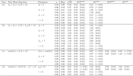
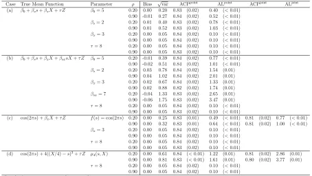
Table 2.1: Simulation results using bootstrap of subject-level residuals and 95% nominal level; results are based on 500 MC samples.

Case True Mean Function Parameter ρ Bias √var ACPpoint

ALpoint

ACPjoint

ALjoint (a) β0+βss+βxX+τ Z β0= 5 0.20 0.00 0.20 0.94 (0.01) 0.54 (<0.01)

0.90 -0.01 0.27 0.94 (0.01) 0.70 (<0.01) βs= 2 0.20 0.01 0.40 0.94 (0.01) 1.06 (<0.01)

0.90 0.01 0.52 0.94 (0.01) 1.39 (0.01) βx= 3 0.20 0.00 0.05 0.95 (0.01) 0.14 (<0.01)

0.90 0.00 0.05 0.95 (0.01) 0.14 (<0.01) τ= 8 0.20 0.00 0.05 0.93 (0.01) 0.14 (<0.01) 0.90 0.00 0.05 0.93 (0.01) 0.14 (<0.01) (b) β0+βss+βxX+βsxsX+τ Z β0= 5 0.20 -0.01 0.39 0.93 (0.01) 1.04 (<0.01) 0.90 -0.02 0.51 0.94 (0.01) 1.36 (0.01) βs= 2 0.20 0.03 0.78 0.93 (0.01) 2.07 (0.01)

0.90 0.04 1.02 0.94 (0.01) 2.72 (0.01) βx= 3 0.20 0.02 0.67 0.93 (0.01) 1.08 (0.01)

0.90 0.02 0.88 0.93 (0.01) 2.36 (0.01) βsx= 7 0.20 -0.04 1.33 0.92 (0.01) 3.60 (0.02)

0.90 -0.06 1.75 0.93 (0.01) 4.71 (0.02) τ= 8 0.20 0.00 0.05 0.93 (0.01) 0.14 (<0.01)

0.90 0.00 0.05 0.93 (0.01) 0.14 (<0.01)

(c) cos(2πs) +βxX+τ Z f(s) = cos(2πs) 0.20 0.00 0.25 0.93 (0.01) 0.67 (<0.01) 0.92 (0.01) 0.95 (<0.01)

0.90 0.00 0.32 0.93 (0.01) 0.87 (<0.01) 0.93 (0.01) 1.23 (<0.01) βx= 3 0.20 0.00 0.05 0.95 (0.01) 0.14 (<0.01)

0.90 0.00 0.05 0.95 (0.01) 0.14 (<0.01) τ= 8 0.20 0.00 0.05 0.93 (0.01) 0.14 (<0.01) 0.90 0.00 0.05 0.93 (0.01) 0.14 (<0.01) (d) cos(2πs) + 4((X/4)−s)3_{+τ Z µ}

4(s, X) 0.20 0.00 0.61 0.94 (<0.01) 1.65 (0.01) 0.93 (0.01) 3.23 (0.01) 0.90 0.00 0.81 0.94 (<0.01) 2.18 (0.02) 0.93 (0.01) 4.26 (0.01) τ= 8 0.20 0.00 0.05 0.93 (0.01) 0.14 (<0.01)

0.90 0.00 0.05 0.94 (0.01) 0.14 (<0.01) Standard errors are presented in parentheses.

rejection probabilities increase with the sample size. Our investigation indicates that the strength of the correlation between the functional observations corresponding to the same subject affect the rejection probability: the weaker the correlation, the larger the power. There is no competitive testing method available for this null hypothesis.

Table 2.2: Empirical Type I error of the test statistic T based on the Nsim = 1000 MC samples.

µ(s, x) = cos(2πs),τ= 0

α= 0.05 α= 0.10 α= 0.15

n= 100 ρ= 0.2 0.08 (0.01) 0.14 (0.01) 0.21 (0.01)

ρ= 0.9 0.09 (0.01) 0.14 (0.01) 0.20 (0.01)

n= 200 ρ= 0.2 0.07 (0.01) 0.13 (0.01) 0.17 (0.01)

ρ= 0.9 0.08 (0.01) 0.12 (0.01) 0.18 (0.01)

n= 300 ρ= 0.2 0.06 (0.01) 0.11 (0.01) 0.16 (0.01)

ρ= 0.9 0.06 (0.01) 0.12 (0.01) 0.16 (0.01)

µ(s, x) = cos(2πs),τ= 8

α= 0.05 α= 0.10 α= 0.15

n= 100 ρ= 0.2 0.07 (0.01) 0.15 (0.01) 0.20 (0.01)

ρ= 0.9 0.08 (0.01) 0.15 (0.01) 0.21 (0.01)

n= 200 ρ= 0.2 0.07 (0.01) 0.13 (0.01) 0.17 (0.01)

ρ= 0.9 0.08 (0.01) 0.12 (0.01) 0.18 (0.01)

n= 300 ρ= 0.2 0.06 (0.01) 0.11 (0.01) 0.16 (0.01)

ρ= 0.9 0.06 (0.01) 0.12 (0.01) 0.16 (0.01) Standard errors are presented in parentheses.

Figure 2.6: Estimated power curves for testing H0 : µ(s, x) = η(s) using level of sig-nificance α = 0.05, when the true mean function µ(s, x) = 2 cos(2πs) +δ(x/4−s)3 _for

Chapter 3

Longitudinal Functional Data

Analysis

3.1

Introduction

Existing literature in longitudinal functional data can be separated into two cate-gories, based on whether or not it accounts for the actual time tij at which the profile

Yij(·) is observed; here i indexes the subjects and j indexes the repeated measures of the subject. Moreover, most methods that incorporate the timetij focus on modeling the process dynamics (Greven et al., 2010) and only few can do prediction of a future full tra-jectory. Chen & M¨uller (2012) considered the latter issue and introduced an interesting perspective, but their method is very computationally expensive and its application in practice is limited as a result. We propose a novel parsimonious modeling framework to study the process dynamics and prediction of future full trajectory in a computationally feasible manner.

In this chapter we focus on the case where the sampling design oftij’s is sparse (hence

sparse longitudinal design) and the subject profiles are observed at fine grids (hencedense functional design). We propose to model Yij(·) as:

Yij(s) =µ(s, tij) +Xi(s, tij) +ij(s); Xi(s, tij) = X k≥1

ξik(tij)φk(s) for s∈ S and tij ∈ T (3.1) where S and T are closed compact sets, µ(·, tij) is an unknown smooth mean response corresponding to tij, Xi(·, tij) is a smooth random deviation from the mean at tij, and

ij(·) is a residual process with zero-mean and unknown covariance function to be de-scribed later. The bivariate processesXi(·,·)’s are independent and identically distributed (iid), the error processes ij’s are iid and furthermore are independent of Xi’s. For iden-tifiability we require that Xi comprises solely the random deviation that is specific to the subject; the repeated time-specific deviation is included in ij. Here {φk(·)}k is an orthogonal basis in L2_{(S) and ξ}

visit times of all subjects, {tij :i, j}, is dense in T. Full model assumptions are given in Section 3.2.

The class of model (3.1) is rich and includes many existent models, as we illustrate now. (i) Ifξik(tij) = ζ0,ik+tijζ1,ik for appropriately defined random termsζ0,ik and ζ1,ik, model (3.1) can be represented as in Greven et al. (2010). (ii) If cov(ξik(t), ξik(t0)) =

λkρk(|t−t0|;ν) for some unknown variance λk, known correlation function ρk(·;ν) with unknown parameter ν, and n= 1, model (3.1) resembles to Gromenko et al. (2012) and Gromenko & Kokoszka (2013) for spatially indexed functional data. (iii) If ξik(tij) = P

l≥1ζiklψikl(tij) with orthogonal basis functions ψikl(t)’s and the corresponding coeffi-cientsζikl’s, then model (3.1) is similar to Chen & M¨uller (2012) who used time-varying basis functionsφk(·|t) instead of our proposedφk(·) in model (3.1) and assumed a white noise residual process ij.

The use of time-invariant orthogonal basis functions is one key difference between the proposed framework and Chen & M¨uller (2012); another important difference is the flexible error structure that our approach accommodates. The key difference leads to several major advantages of the proposed method. First, by using a time-invariant basis functions, the basis coefficients, ξik(tij)’s extract the low dimensional features of these massive data. The longitudinal dynamics is emphasized only through the time-varying coefficients ξik(tij)’s of (3.1) and, thus, this perspective makes the study of the process dynamics easier to understand. Second, our approach involves at most two dimensional smoothing and as a result is computationally very fast; in contrast, the time-varying basis functions {φk(·|t)}k at each t, require three dimensional smoothing which is not only complex but also computationally intensive and slow.

of sparse functional data. Another option is to use data-driven basis functions, such as eigenbasis of some covariance. The challenge is: what covariance to use? We take the latter direction and propose to determine {φk(·)}k using an appropriate marginal covariance. In this regard, let c((s, t),(s0, t0)) be the covariance function of Xi(s, t) and g(t) be the density of tij’s. Define Σ(s, s0) =

R

T c((s, t),(s

0_{, t))g(t)dt for s, s}0 _{∈ S: we show that this} bivariate function is a proper covariance function (Horv´ath & Kokoszka, 2012). Section 3.2 shows that the proposed basis {φk(·)}k has optimal properties with respect to some appropriately defined criterion. From this view point, the model representation (3.1) is optimal. The idea of using the eigenbasis of the pooled covariance can be related to Jiang & Wang (2010) and Pomann et al. (2013), who considered independent functional data. The rest of the chapter is organized as follows. Section 3.2 introduces the proposed modeling framework. Section 3.3 describes the estimation methods and implementation. The methods are studied theoretically in Section 3.5 and then numerically in Section 3.6. Section 3.7 discusses the application to the tractography DTI data.

3.2

Modeling longitudinal functional data

Let [{tij, Yij(sr) :r = 1, . . . , R}:j = 1, . . . , mi,] be the observed data for theith subject, whereYij(·) is thejth profile at random timetij for subjecti, and each profile is observed at the fine grid of points {s1, . . . , sR}. For convenience we use the generic indexsinstead ofsr. The number of ‘profiles’ per subject,mi is relatively small to moderate and the set of time points of all subjects,{tij : for all i, j}, is dense inT. Without loss of generality, we set S = T = [0,1]. We model the response Yij(·) using (3.1), where we assume that