Models of Frequency-Dependent Selection with Mutation from Parental Alleles

(1)

INVESTIGATION

Models of Frequency-Dependent Selection with

Mutation from Parental Alleles

Meredith V. Trotter*,1_{and Hamish G. Spencer}†

*Department of Biology, Stanford University, Stanford, California 94305 and†Allan Wilson Centre for Molecular Ecology and Evolution, Department of Zoology, University of Otago, Dunedin 9054, New Zealand

ABSTRACTFrequency-dependent selection (FDS) remains a common heuristic explanation for the maintenance of genetic variation in natural populations. The pairwise-interaction model (PIM) is a well-studied general model of frequency-dependent selection, which assumes that a genotype’sfitness is a function of within-population intergenotypic interactions. Previous theoretical work indicated that this type of model is able to sustain large numbers of alleles at a single locus when it incorporates recurrent mutation. These studies, however, have ignored the impact of the distribution offitness effects of new mutations on the dynamics and end results of polymorphism construction. We suggest that a natural way to model mutation would be to assume mutantfitness is related to the

ﬁtness of the parental allele,i.e., the existing allele from which the mutant arose. Here we examine the numbers and distributions of

fitnesses and alleles produced by construction under the PIM with mutation from parental alleles and the impacts on such measures due to different methods of generating mutantfitnesses. Wefind that, in comparison with previous results, generating mutants from existing alleles lowers the average number of alleles likely to be observed in a system subject to FDS, but produces polymorphisms that are highly stable and have realistic allele-frequency distributions.

I

T has been nearly 50 years since molecular techniquesﬁrst revealed the ubiquity of genetic variation in nature (Hubby and Lewontin 1966). Neutral theories of the maintenance of variation (Ohta 1973; Kimura 1984) remain the dominant framework underlying most population-genetic models, but we now know that most, if not all, genetic variation is subject to some degree of natural selection (Hahn 2008). Despite a rich theoretical and empirical literature on the subject, how-ever, pinning down the mechanisms that allow selective main-tenance of genetic variation remains a stubborn challenge

(Lefﬂeret al.2012).

Early theoretical work in this area focused on the mainte-nance of diallelic polymorphisms (e.g., Levene 1953; Li 1955; Lewontin 1958; Haldane and Jayakar 1963;Hedrick 1986),

largely for mathematical convenience. Unfortunately, the results of diallelic approaches quite often do not scale up to the multiallelic case in intuitive or analytically tractable ways (Gillespie 1977;Lewontinet al.1978;Karlin 1981;Clark and

Feldman 1986;Matessi and Schneider 2009;Muirhead and

Wakeley 2009; Nagylaki 2009; Schneider 2009; Waxman

2009). Empirical studies conﬁrm that nonneutral polymor-phisms with more than two alleles are very common (Keith 1983; Keithet al.1985; Bradleyet al.1993; Moriyama and Powell 1996; Hahn 2008). MHC loci, to name one extreme example, can have hundreds of alleles (for a review, see Garrigan and Hedrick 2003).

The standard approach to modeling the maintenance of selected polymorphism—what we call the“parameter-space approach”—has been to generate large numbers of ﬁtness sets, either randomly (Lewontinet al.1978; Clark and Feldman 1986; Asmussen and Basnayake 1990; Gimelfarb 1998) or us-ing some preselected patterns (Karlin 1981), to systematically search the available parameter space to assess which selection regimes and what proportion of parameter space maintain var-iation for a given number of alleles. This proportion is inter-preted as an estimate of the “potential”for variation under a given selection regime. These types of models have typically found that the proportion of randomly generatedﬁtness sets that maintain variation becomes vanishingly small forn.5 alleles if viability is assumed to be constant (Gillespie 1977; Lewontinet al.1978); the same holds true in models of con-stant fertility selection (Clark and Feldman 1986).

Manuscript received April 23, 2013; accepted for publication July 2, 2013 Supporting information is available online athttp://www.genetics.org/lookup/suppl/ doi:10.1534/genetics.113.152496/-/DC1.

1_{Corresponding author: Department of Biology, Stanford University, Gilbert Biological}

(2)

It is far more biologically reasonable to expect selection pressures to change in space or time, however (Kojima 1971). Modern hypotheses to explain selective polymorphism have included heterozygote advantage (e.g., Kekäläinenet al.

2009; Spurgin and Richardson 2010; Selliset al.2011), spa-tially heterogeneous selection (e.g., Hedrick 1986; Staret al.

2007a,b; Nagylaki 2009), and sexual antagonism (Curtsinger

et al.1994; Foersteret al.2007; Hallet al.2010; Mokkonen

et al. 2011; Connallon and Clark 2012). Nevertheless, the

most common heuristic invoked to explain nonneutral varia-tion in natural systems remains frequency-dependent selec-tion (FDS) (see Sinervo and Calsbeek 2006 for a review).

FDS describes any selection regime where a genotype’s fitness depends on the frequencies of its own or other geno-types in the population. Negative frequency dependence (se-lection in favor of rare alleles) is often invoked to explain polymorphism, since if it is beneficial to be rare, it is also difficult to go extinct. Conversely, positive frequency depen-dence (selection in favor of common alleles) is expected to eliminate variation. It is important to note that simple positive FDS and negative FDS are extremes at opposite ends of a con-tinuum. Intraspecific interactions such as mate choice (e.g., Hughes et al. 1999) and alternative mating strategies (Sinervo and Lively 1996) have been shown to produce both negative and positive FDS, sometimes both within the same population (see Sinervo and Calsbeek 2006 for a review). In-terspecific interactions such as mimicry (e.g., Borer et al.

2010), host–parasite coevolution(Dybdahl and Lively 1998;

Koskella and Lively 2009), and predator–prey dynamics (e.g., Olendorfet al.2006;Marples and Mappes 2010) can produce

negative FDS, positive FDS, and other more nuanced FDS regimes. The diversity of FDS regimes observed in nature suggests that any investigation of the potential for genetic variation under FDS should use a very general model.

Here we restrict ourselves to the study of FDS that results from intraspecific interactions. The most general model of this kind of FDS is the discrete-time pairwise-interaction model (PIM) (Cockerhamet al.1972), which parameterizesfitness as a product of intraspecific competition at the genotype level. This approach provides a biologically reasonable way to model frequency-dependent viabilities, conceptually similar to the payoff matrix of evolutionary game-theoretic models (Maynard Smith 1982). The wildcard model of FDS (Matessi and Schneider 2009 and references therein) is a continuous-time analog to the PIM in the specific case of symmetricfitness interactions. The wildcard model leads to several useful

results for multiple alleles (see Schneider 2009), but the re-quirement of symmetric interactions limits its generality. We are interested in exploring the full parameter space of frequency-dependent selective scenarios, and for our purposes the discrete-time PIM provides the most general framework available.

In the PIM each genotype is assumed to have a constant interactionfitness with every other genotype in the popula-tion. Assuming random mixing of individuals, the frequencies of interactions are given by the product of the frequencies of the interacting genotypes, and the totalfitness of a genotype is a weighted sum of its fitnesses in interactions with all genotypes. This general formulation allows the PIM to parameterize a wide range of FDS regimes (positive, negative, balancing, and disruptive), as well as constant selection as a special case. A recent investigation of the potential for polymorphism under the PIM, using the parameter-space approach, found that FDS has a higher potential for variation than the equivalent constant viability model for any given number of alleles (Trotter and Spencer 2007). It was also found that a wide variety of flavors of FDS, not simply negative FDS, have potential for polymorphism under the PIM.

The traditional parameter-space approach, while infor-mative, ignores the process of mutation and invasion that necessarily underlies the development of any natural poly-morphism. An alternative, the so-called“constructionist” ap-proach to modeling the maintenance of genetic variation, is analogous to some models of ecological community construc-tion (Nee 1990). In a construcconstruc-tionist model, polymorphisms (communities) develop from monomorphisms (single spe-cies). New mutant alleles (species) are introduced at a set rate of mutation (migration) and allowed to invade or be repulsed by the existing system based on their relativeﬁtnesses. Early constructionist models of genetic variation found that con-stant viability can easily generate intermediate numbers of alleles (Spencer and Marks 1988, 1992; Marks and Spencer 1991). A recent model of polymorphism construction using the PIM (Trotter and Spencer 2008) found FDS with recurrent mutation can result in very high levels of single-locus polymorphism.

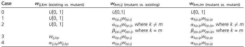
A deﬁning feature of this last model was the assumption that new mutant interactionﬁtnesses be drawn from a uni-form distribution on [0, 1]. However, this method ignores the reality that new mutations result from changes (usually small) to an existing allele. This relationship suggests a more Table 1 Guide to the cases of the PIM

Case wij,km(existingvs.mutant) wkm,ij(mutantvs.existing) wkm,im(mutantvs.mutant)

0 U[0, 1] U[0,1] U[0, 1]

1 U[0, 1] akp,ijwkp,ij akp,ipwkp,ip

2 U[0, 1] akp,ijwkp,ij, wherek6¼m akp,ipwkp,ip, wherek6¼m

bpp,ijwpp,ij, wherek=m bpp,ipwpp,ip, wherek=m

3 wij,kp akp,ijwkp,ij akp,ipwkp,ip

(3)

natural way to model mutants arising from within the population might be to have mutant fitnesses be some function of thefitness of a“parental”allele from which they descend. Because the vast majority of new mutations are neu-tral or weakly deleterious (Eyre-Walker and Keightley 2007), simulated mutants should be on average similar to, but lessfit than, their parental allele. The model of Spencer and Marks (1992) incorporated mutation from existing alleles (parental allele,Ap, mutated to a novel allele,Am) in a constructionist

approach to modeling the maintenance of variation by con-stant viability selection. In their models, the viabilities of mu-tant AiAm genotypes (wim) were drawn from distributions

centered just below theﬁtness of the equivalent parental ge-notypeAiAp(wip); hence most mutants were slightly

deleteri-ous. In this study, we incorporate mutation from existing alleles into constructionist approaches, using the PIM of FDS.

Models

We model selection acting on a large, isolated, randomly mating monoecious population of diploid organisms with nonoverlapping generations. Under the PIM, each genotype

AiAjhas constantﬁtnesses (wij,kl) in its interactions with the

other genotypesAkAlin the population (i,j,k,l= 1, 2,. . ., n). These interactionfitnesses collectively define thefitness

set. We assume AiAjis equivalent to AjAi, and so wij,kl = wji,kl=wij,lk=wji,lk.

When adding a new allele to ann-allele system with PIM fitnesses, there are several different types of interactions that need to be parameterized and (n+ 1)3_{new interaction} fitnesses that must be generated. This extra dimension of fitness makes linking mutant fitnesses to a parental allele a more complicated endeavor. The addition of a new allele,

An+1, results inn +1 new genotypes, each of which must be assigned interactionﬁtnesses for their interactions with the

nðnþ1Þ=2 existing genotypes and then+ 1 new genotypes. We refer to these interaction fitnesses as the mutant fi t-nesses. In addition, each existing genotype must also be givenn+ 1 new interactionfitnesses, corresponding to their interactions with each of the new genotypes. We refer to these as the mutant impacts, as they represent the change to the fitnesses of existing genotypes due to their interac-tions with the new mutant. The number of elements in the updated fitness set, the sum of the number of mutant fi t-nesses and impacts therefore, is

ðnþ1Þ

nðnþ1Þ

2 þ ðnþ1Þ

þ

nðnþ1Þ 2

ðnþ1Þ¼ðnþ1Þ3:

We use four separate cases of the PIM construction model, as detailed below, to investigate the consequences of different methods of generating mutantfitnesses and mutant impacts. Thefirst two cases illustrate the effects of generating mutant fitnesses related to a given existing allele’sfitnesses. The sec-ond pair of cases illustrates the additional changes in model behavior resulting from generating mutant impacts related to the existing impacts of a given parental allele. For all cases, we are interested in the levels and stability of polymorphism and distributions offitness produced by construction under the PIM with mutation from existing alleles and the impacts on such measures due to the different methods of generating fitnesses.

The constructionist approach to modeling selection has three stages each generation: mutation, selection, and extinction check.

Mutation

Every generation, an allele existing in the population is chosen to mutate. (For the effects of different mutation rates, seeFile S1.) The probability of a given allele (Ai) being chosen

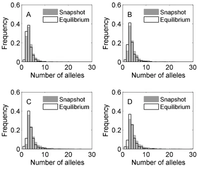
Figure 1 Numbers of alleles present at snapshot (shaded) and at equi-librium (open) in 1000 runs each for all cases of PIM construction. A–E represent cases 0–4 in order.

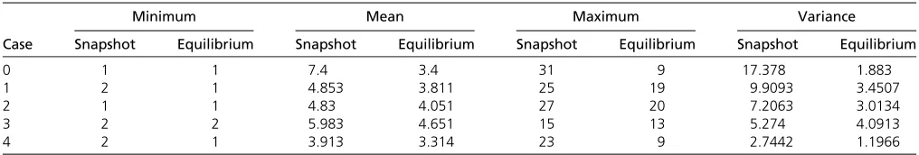
Table 2 Summary statistics for numbers of alleles present at snapshot and equilibrium taken across 1000 runs each of all cases of PIM

Minimum Mean Maximum Variance

Case Snapshot Equilibrium Snapshot Equilibrium Snapshot Equilibrium Snapshot Equilibrium

0 1 1 7.4 3.4 31 9 17.378 1.883

1 2 1 4.853 3.811 25 19 9.9093 3.4507

2 1 1 4.83 4.051 27 20 7.2063 3.0134

3 2 2 5.983 4.651 15 13 5.274 4.0913

(4)

as a “parent”allele is proportional to its frequency in the population,pi. The frequency of the parental allele (Ap) is then

decremented by 1026and the mutant allele (Am, wherem= n+ 1) is introduced at frequency of 1026. We assume this implied population size ofN= 53105_{is large enough to} ignore the effects of random drift. New interactionfitnesses are added to thefitness set in three stages. First, the preexist-ing genotypes (AiAj) are assignedfitnesses in their interactions

with the new mutant genotypes (AkAm). These ﬁtnesses, wij,km, represent the“impact”of the new mutant on theﬁtness

of existing genotypes. Second, the new mutant genotypes are assigned ﬁtnesses in their interactions with the preexisting genotypes,wkm,ij. Finally, the mutant genotypes are assigned

ﬁtnesses in their interactions with the other mutant geno-types,wim,km.

We investigatedfive different methods for generating the required new interactionfitnesses after the addition of mutant alleles. A summary of the methods of generatingfitnesses used in each case can be found in Table 1.

General case

In the general form of the model, hereafter referred to as case 0, all new interactionﬁtnesses are drawn from the uniform distribution on [0, 1]. This method implies independence between theﬁtnesses of the parental and mutant alleles and the impact of the new allele on existing genotypes. The data shown for this case are taken from Trotter and Spencer

(2008) and are used as the basis for comparison for the other cases.

Case 1

Empirical data suggest that the majority of new mutations are slightly deleterious (Mukaiet al.1966; Eyre-Walker and Keightley 2007). Consequently, in all further cases we model mutant ﬁtnesses (wkm,ij) to be, on average, slightly lower

than the equivalent parentalﬁtness. In thisﬁrst case of mu-tation from existing alleles, we continue to draw thewij,km

impacts from the uniform distribution on [0, 1]. Each new mutant interactionﬁtness (wkm,ij), however, is now a

func-tion of the existing interacfunc-tion ﬁtness (wkp,ij) of the

corre-sponding parental genotype (AkAp) and is given by

akp,ijwkp,ij. We draw theafrom a rescaled beta-distribution

on [0, 1.5] that is conditioned to have meanmaand variance s2

a. Note that a new, independent,ais drawn for every new mutant interactionﬁtness. For all our cases, we set 0,ma, 1 and assumes2

ato be small. By rescaling the distribution ofain this way, we avoid negativefitnesses, but beneficial mutations (a.1) remain possible but rare. In case 1, we set ma= 0.95,s2a= 0.001, to produce primarily mutations of moderately negative effect, with rare beneficial mutations (,5%). (For details of the effects of varying ma and s2a see File S1.)

We set homozygous mutantsAmAmto be lethal with

(5)

this rare lethality produce nearly identical outcomes of poly-morphism construction; seeFile S1.) In the case of lethality, all wmm,ij= 0; otherwise homozygote ﬁtnesses are

gener-ated using the same method for all other wkm,ij.

Case 2

A previous model of mutation from existing alleles (Spencer and Marks 1992) assumed that heterozygote and homozy-goteﬁtnesses are drawn from slightly different distributions (with heterozygotes being, on average,ﬁtter than homozy-gotes). For purposes of direct comparison with that model, we here recreate it using our PIM approach. We continue to draw thewij,kmimpacts from the uniform distribution on [0,

1]. Each mutant interaction ﬁtness (wkm,ij) is a function of

the existing interaction ﬁtness (wkp,ij) of the corresponding

parental genotype (AkAp) and is given byakp,ijwkp,ij, where

eachais drawn from a rescaled beta-distribution on [0, 1.5] withm_a¼0:95;s2

a¼0:001 for heterozygotes (i.e., whenk6¼

m), and bybkp,ijwkp,ij, where eachbis drawn from a rescaled

beta-distribution on [0, 1.5] with m_b¼0:9;s2

b¼0:002 for homozygotes (i.e., whenk=m).

Case 3

In this case, as in case 1, both homozygote and heterozy-gote mutant ﬁtnesses are functions of the existing in-teraction ﬁtness (wkp,ij) of the corresponding parental

genotype (AkAp) and are given by akp,ijwkp,ij, where each

a is drawn from a rescaled beta-distribution on [0, 1.5] with m_a¼0:95;s2

a¼0:001. We know from the general construction PIM for FDS (Trotter and Spencer 2008) that the impacts, thewij,km, greatly affect the likelihood of allele Amsuccessfully invading the polymorphism. A mutant allele

that leads to low values ofwij,kmwill drag down theﬁtnesses

of existing alleles, thereby improving its own chances of in-vading the polymorphism. In this case, instead of drawing the

wij,kmfrom the uniform distribution, we assume thewij,kmare

strictly equal to the impacts of the parental allelewij,kp.

Case 4

In this case, instead of thewij,kmbeing strictly equal to the

equivalent parentalfitness, we assume they have, on aver-age, a slightly deleterious effect on existing genotypes. This deleterious effect is accomplished by setting all new in-teractionfitnesses as functions of the existing interaction fitness (wkp,ij) of the corresponding parental genotype

(AkAp) and is given by akp,ijwkp,ij, where each aijk is

drawn from a rescaled beta-distribution on [0, 1.5] with m_a¼0:95;s2

a¼0:001. As a result, this case produces mu-tant alleles that have low ﬁtness, but that are also good invaders. This case is motivated less by biological realism (we know of no reason to expect mutations to be biased in favor of negative impacts in this way) and more as a test of whether a mutant’sﬁtnesses, or its impact on other geno-types, are more important to invasion success.

Selection and extinction

Overall genotypic ﬁtnesses, wij, are linear functions of the

interaction ﬁtnesses with all other genotypes in the model, weighted by the frequencies of all interacting genotypes:

wij¼ Xn

k¼1 Xn

l¼1

pkplwij;kl:

The marginal ﬁtness of alleleAiis the sum ofﬁtnesses for

all genotypes involving Ai, weighted by their frequencies:

wi¼

Pn j¼1pjwij.

After the mutantﬁtnesses have been added to theﬁtness set, allele frequencies are updated according to the standard population genetics equation

p_i9¼piwi

w ; (1)

where piis the frequency of alleleiat generationt, andw

is the mean ﬁtness of the population at generation t. The change in allele frequency after selection is thus Dp¼pi92pi. After allele frequencies are updated, alleles

whose frequencies fall below 1026(our implied 1/2N) are considered to be extinct and are removed from the system. Each model run was initialized with a single allele with ﬁtnesswi¼0:5. Each generation we recorded the numbers,

Figure 3 Close-up of an example of meanﬁtness oscillations from case 3 data. Cases 1–4 all occasionally produce these kinds of qualitatively re-petitive dynamics.

(6)

ages, and frequencies of all alleles and also the meanfitness. After 10,000 such generations had passed, we recordedfi t-ness sets, as well as numbers and frequencies of alleles. Since FDS construction systems do not converge to a steady state (see Trotter and Spencer 2008), we wanted to run the muta-tion process for long enough to avoid sampling during the initial transient period, but not so long that assuming selection to be consistent for that many generations is unreasonable. The mutation process was halted after 10,000 generations and the system was allowed to continue iterating to equilibrium (defined as either a monomorphic equilibrium or a polymorphic equilib-rium with |Δpi|,1028for alli). At equilibrium,final

measure-ments of the numbers, ages, and frequencies of alleles and the meanﬁtness were recorded. The equilibrium statistics indicate how much of the“snapshot”variation is transient and how much is likely to be permanent, as well as providing a means of com-paring the results of the construction approach with those of earlier parameter-space approaches. For each case, 1000 repli-cate runs, differing only in the pseudorandom number seed, were performed.

Results

Allele numbers

Distributions of numbers of alleles present at snapshot and at equilibrium for all cases are shown in Figure 1, and

summary statistics for these distributions are found in Table 2.

In all cases, the model produced an initial transient increase and subsequent crash inn, followed by perpetual ﬂuctuations (Figure 2). In all cases, at least 99% of runs had$2 alleles at snapshot, while at equilibrium monomor-phism was rare but possible (0.1–3% of runs). Case 4 pro-duced snapshot polymorphisms with smallest average n

(3.9 alleles), which is unsurprising since its mutation pro-cess draws all new interactions from distributions centered below the mean of existingﬁtnesses. Case 1 generated on average more alleles than case 2, despite case 2 having built-in heterozygote advantage. This trend is counter to the intuitive idea that, all else being equal, heterozygote advantage promotes polymorphism. Case 3 typically generated snapshot polymorphisms with the most alleles (6 on average).

Meanﬁtness

Examples of the trajectories of mean fitness and allele number from all cases are illustrated in Figure 2. Each case occasionally (but rarely) producedfluctuating meanfitness trajectories such as those shown in Figure 3. During these fluctuations, while n remains constant the mean fitness decreases to some threshold, at which point multiple inva-sions occur and the meanfitness rebounds. A sharp spike in mean fitness often coincides with multiple extinctions as a highlyfit allele drives others out.

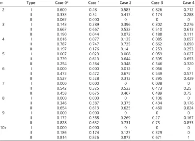
Table 3 The proportion of simulations leading to type I, II, or IIIﬁtness sets for each PIM construction model, listed by snapshotn

n Type Case 0a Case 1 Case 2 Case 3 Case 4

2 I 0.600 0.48 0.583 0.826 0.712

II 0.333 0.52 0.417 0.174 0.288

III 0.067 0.000 0 0 0

3 I 0.143 0.289 0.396 0.302 0.276

II 0.667 0.667 0.532 0.510 0.613

III 0.190 0.044 0.072 0.188 0.111

4 I 0.016 0.077 0.135 0.085 0.057

II 0.787 0.747 0.725 0.662 0.690

III 0.197 0.176 0.14 0.253 0.253

5 I 0.007 0.023 0.008 0.059 0.027

II 0.739 0.613 0.644 0.595 0.653

III 0.254 0.364 0.348 0.346 0.320

6 I 0.000 0.000 0.012 0.056 0

II 0.473 0.472 0.675 0.549 0.571

III 0.527 0.528 0.313 0.395 0.429

7 I 0.000 0.000 0 0.038 0

II 0.542 0.325 0.533 0.473 0.25

III 0.458 0.675 0.467 0.489 0.75

8 I 0.000 0.000 0 0.106 0

II 0.346 0.387 0.375 0.434 0.176

III 0.654 0.613 0.625 0.460 0.824

9 I 0.000 0.000 0 0 0

II 0.172 0.368 0.269 0.27 0.167

III 0.828 0.632 0.731 0.73 0.833

10+ I 0.000 0.000 0 0 0

II 0.186 0.174 0.127 0.329 0

III 0.814 0.826 0.873 0.671 1

(7)

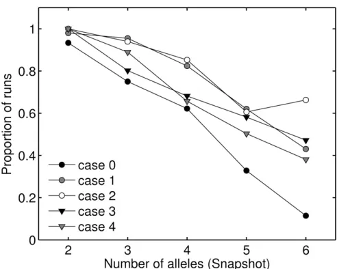
Potential for polymorphism

The potential for polymorphism has been deﬁned as the proportion of random initial allele frequencies and ﬁtness sets that maintain all alleles under a given model (Lewontin

et al.1978;Asmussen and Basnayake 1990;Asmussenet al.

2004;Staret al.2007a;Trotter and Spencer 2007, 2008). In

the context of construction approaches, we measure poten-tial as the proportion of model runs that maintained all alleles present at snapshot, at equilibrium. All four muta-tion-from-existing-alleles cases had a higher proportion of runs maintain all snapshot alleles than did the general case (see Figure 4). We see in Figure 4 that cases 3 and 4 appear to have slightly lower potential than cases 1 and 2 as n

increases. Case 2 had an unusually large number of runs (83), maintaining six alleles at equilibrium.

Another method of measuring the potential for variation is to iterate each snapshot ﬁtness set to equilibrium from many starting allele-frequency vectors (Star et al. 2007b). The proportion of vectors that maintain all snapshot alleles for a particularﬁtness set gives a measure of the domain of

attraction of the fully polymorphic equilibrium for that set.

Staret al.(2007b) used this method to partition their

equi-librium fitness sets into three classes: type I fitness sets maintain full polymorphism from all initial conditions and can be considered to have globally stable equilibria; type II fitness sets maintain all alleles from only a subset of all start vectors and thus have locally stable equilibria; and type III fitness sets lose at least one allele from all initial conditions, implying that some of the snapshot polymorphism is always transient. Numbers of type I, II, and IIIfitness sets from all PIM construction cases can be found in Table 3. In all cases, asnincreases the proportion of type Ifitness sets drops off dramatically. No type Ifitness sets were found forn.8. The proportion of type I polymorphisms drops off more slowly in case 3 than in other cases. Based on this measure of poten-tial, then, case 3 appears to produce polymorphisms with larger domains of attraction.

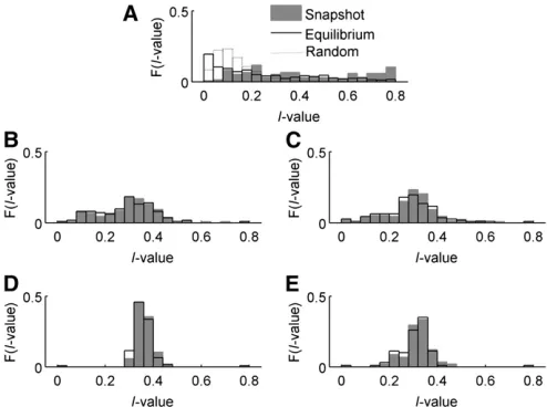
Allele-frequency distributions

For each case, we compared the allele-frequency distri-butions present at snapshot and at equilibrium, using

I¼Pni¼1ðpi21 = nÞ2, the sum of squared deviations of allele

frequencies from the centroid of allele-frequency space, as a measure of their centrality. If all alleles in the distribution are present at equal frequency, eachpiwill be 1/nand thus I= 0. If one allele is common and the others are vanishingly rare,Iﬃ ðn21Þ = n. In natural systems, truly centered allele-frequency distributions are rare (Keith 1983; Keith et al.

1985), and thus the ability of any model to generate skewed distributions reflects its biological plausibility. Distributions ofI-values from allele-frequency equilibria forn= 5 gener-ated by the different cases are summarized in Figure 5. We focus on the case of n =5 in many of our analyses for two reasons. First,five alleles was the outcome between 7% and 13% of the time in both snapshot and equilibrium results, giving this case a sample size of100 replicates for all cases. Second, and more importantly forfitness analyses,n= 5 is the smallest polymorphism that includes all possible inter-genotypic interactions (see Trotter and Spencer 2007 for a discussion of the special properties of PIM when n= 2, 3, and 4).

Figure 5 Frequency plots ofI-values for all cases. Shaded area, snapshot results withﬁve alleles; solid line, equilibrium results withﬁve alleles. The dotted line in case 0 indicates the expected distribution ofI-values for random allele frequencies. A–E represent cases 0–4 in order.

Table 4 Correlations betweenCclass values and potential to maintain snapshot variation at equilibrium

Case 0 Case 1 Case 2 Case 3 Case 4

Fitness class rs P rs P rs P rs P rs P

Cii,ii 20.184* 0.033 20.248** 0.005 20.291** 0.001 0.013 0.871 20.020 0.809

Cii,jj 0.044 0.615 20.005 0.955 0.109 0.214 0.033 0.688 0.015 0.861

Cii,ij 0.051 0.559 20.360** 0.000028 20.110 0.211 0.035 0.666 0.039 0.641

Cii,jk 0.559 0.922 20.008 0.928 0.293** 0.0006 0.004 0.961 0.064 0.442

Cij,jj 20.194* 0.025 20.245** 0.005 20.319** 0.00019 0.023 0.774 0.186* 0.024

Cij,kk 20.182* 0.035 20.039 0.664 20.018 0.839 0.270** 0.001 0.433** 0.00000004

Cij,ik 0.063 0.469 20.076 0.391 0.037 0.676 0.117 0.149 0.283** 0.001

Cij,kl 20.011 0.904 0.244** 0.005 0.257** 0.003 0.296** 0.0002 0.436** 0.0000003

Cij,ij 0.173* 0.046 20.363** 0.000023 20.200* 0.021 0.054 0.508 20.042 0.617

(8)

Case 0 had significant differences (P,0.0001) between distributions of snapshot and equilibrium I-values, with equilibrium values shifted toward 0 due to the loss of rare transient alleles. Surprisingly, in cases 1–4 the systems with five alleles at snapshot or at equilibrium produce distribu-tions of I-values that are not significantly different (two-sample Kolmogorov–Smirnov test, P = 0.72, 0.50, 0.25, and 0.59 for cases 1–4, respectively). Equally surprising are the shapes of those distributions. In cases 1–4,I-values show bell-shaped frequency distributions, centered above 0, that do not shift between snapshot and equilibrium. This suggests that these models produce polymorphisms that have skewed distributions (I.0) and are also stable, being less likely to lose transient alleles on the way to equilibrium.

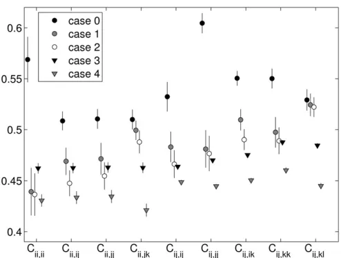
Analysis ofﬁtness sets

Following Trotter and Spencer (2007), we divided the interaction-fitness values within each fitness set into nine fitness“classes”. Class divisions are set based on heterozy-gosity of, and allelic similarities between, the interacting genotypes. Subscripts denote homo- and heterozygosity, as well as allele sharing between interacting genotypes. Let the class of homozygote by unlike-homozygote interactions be

Cii,jj, that of homozygote by like-homozygote interactions be Cii,ii, that of heterozygote by like-heterozygote interactions

be Cij,ij, that of heterozygote by similar heterozygote

inter-actions beCij,jk, that of heterozygote by unrelated

heterozy-gote interactions be Cij,kl, and so forth. For a givenﬁtness

set, each class value takes the mean of all interaction fi t-nesses in that class. The relative values offitness class means can be taken to indicate different forms of frequency depen-dence. For example, we say fitness sets with low values of self–self interactions (Cii,iiandCij,ij) exemplify negative

fre-quency dependence, since low ﬁtness in self-interactions causes lower relativeﬁtness for common alleles.

In this analysis, we again focus on the case wheren= 5. The casesn= 2, 3, and 4 of the PIM do not exhibit allfitness classes (again, see Trotter and Spencer 2007 for further discussion of this issue). For all cases, some snapshotfitness sets maintained all alleles at equilibrium from all initial con-ditions, some from only a few, and some from none at all. One might then expect to find some relationship between the contents of a snapshot fitness set and the size of the domain of attraction of its fully polymorphic equilibrium. For example,fitness sets with heterozygote advantage might keep all alleles more often than dofitness sets with homo-zygote advantage. In a parameter-space approach (Trotter

and Spencer 2007), PIMﬁtness sets with low self-interaction ﬁtnesses (Cii,ii,Cij,ij,Cij,jj,Cii,ij) had larger within-set potential

for variation. We examined correlations between the pro-portion of initial conditions that maintain snapshot variation (P) and allC class values, using Spearman’s nonparametric r(rs). These relationships are summarized in Table 4. While all cases had signiﬁcant correlations betweenPand at least one C, all such correlations are weak. Cases 1 and 2 have signiﬁcant negative correlations between potential and the

homozygote interaction classes (Cii,__) as well as the

hetero-zygote self-self interaction class (Cij,ij). Cases 3 and 4 have

signiﬁcant positive correlations betweenPand most hetero-zygoteﬁtness classes. Thus, cases 1 and 2 show some signal of negative frequency dependence, while cases 3 and 4 seem to show more effects of heterozygote advantage.

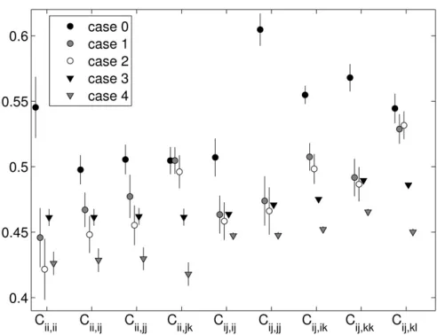
The patterns of fitness produced by cases 1 and 2 agree closely for all fitness classes (see Figures 6 and 7). Case 2 has mild heterozygote advantage built in, so it is surprising that its heterozygotefitnesses are not the highest. Strangely enough, the signal for heterozygote advantage itself is more clearly pronounced in the data from cases 3 and 4, where heterozygote class means are all higher than the correspond-ing homozygote class means (with the exception of the het-erozygote self–self interaction, which is comparatively low in case 3). The trends produced by cases 1 and 2 are more indicative of negative FDS, where self-interaction fitnesses (interactions between genotypes with shared alleles) are minimal (see low values of Cii,ii, Cij,ij, and Cij,jj) with

the exception of those with the least sharing and the most heterozygous,Cij,jk.

Theﬁtness class means from the snapshot data (Figure 6) and in the equilibrium data (Figure 7) are similar, but with higher values in most classes at equilibrium, consis-tent with the loss of low-ﬁtness transient alleles on the way to equilibrium.

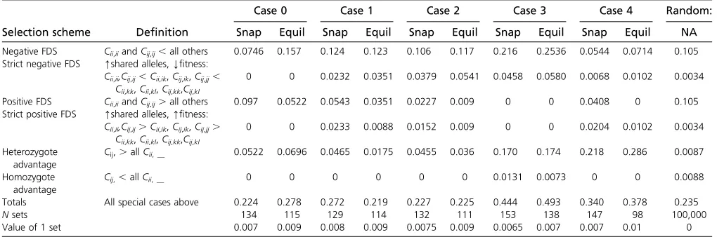
Flavors of frequency dependence

(9)

and positive FDS are equally probable. In the general con-struction model (case 0), we see that positive FDS is slightly more common (10% of sets) than negative FDS (7%) in snapshot, but that this relationship is reversed in the equi-librium sets (5% and 16%). In the simplest mutation-from-existing-alleles model (case 1), all of our definedflavors of FDS occur, with the exception of heterozygote disadvantage. Negative FDS is more common than positive FDS; and het-erozygote advantage is more common than hethet-erozygote disadvantage, which aligns with the usual intuitive under-standing of how FDS should best maintain variation. In cases 1–4, negative FDS is always more common than in the sample of randomly generatedfitness sets, and in cases 2–4 it is more common in equilibrium than in snapshot sets. Positive FDS occurs in all cases except case 3, but it is rare. Heterozygote advantage is very common in cases 3 and 4, but surprisingly not very common in case 2 (which has in-built heterozygote advantage). The addition of defined mu-tant impacts (cases 3 and 4) produces some notable changes. In case 3, negative FDS and heterozygote advantage are both present in20% offitness sets while in case 4, hetero-zygote advantage is common but negative FDS is strikingly rare.

Discussion

In this series of simulations, we have investigated the effect of mutation from existing alleles on the potential for polymorphism under a construction approach to the PIM of FDS. We ﬁnd that generating mutants from existing alleles lowers the average number of alleles found in a system subject to FDS under a construction approach, relative to previously studied models with uniformly dis-tributed mutant ﬁtnesses. Interestingly, while the overall numbers of alleles found at a given time point are lower, the

polymorphisms produced are more stable, with more natural allele-frequency distributions.

Contrary to our intuitive expectation, the cases that were expected to produce more alleles actually had lower overall levels of polymorphism. The case with built-in heterozygote advantage (case 2) produced fewer alleles than the equiv-alent case with all mutant ﬁtnesses drawn from the same distribution (case 1). The case in which mutant impacts are negative (case 4) produced fewer alleles than the case in which mutants are indistinguishable from their parent in terms of their impact on other alleles (case 3). This case, in which mutant impacts are strictly equal to parental impacts, produced the highest mean levels of polymorphism at both snapshot and equilibrium. This case is arguably the most biologically reasonable of the four, since mutants in case 3 are in general lessﬁt than their parental allele, but have no or negligible effect on preexisting alleles. [It is generally accepted that the majority of new mutations are deleterious mutations of small effect, but there is no biological reason to expect that mutants should have deleterious impacts on other genotypes (as in case 4)]. Thus, it is interesting that case 3 produced the highest numbers of alleles.

The PIM is well known to generate decreases in mean ﬁtness (Cockerham et al. 1972; Asmussen and Basnayake

1990; Asmussen et al. 2004; Trotter and Spencer 2007)

and nonmonotonic mean-fitness trajectories (Trotter and Spencer 2009). However, iffitnesses are symmetric (or pseu-dosymmetric, see Matessi and Schneider 2009), the PIM does evolve to maximize mean fitness (or closely related quantities). Earlier construction approaches to the PIM found the mean fitness to be erratic and largely decoupled from the number of alleles (Trotter and Spencer 2008). In most of our simulations of cases 1–4, there were long peri-ods of stable allele number and meanfitness, corresponding to particularly stable arrangements of fitness. However, given that the distributions of mutantfitnesses are functions of parental frequencies, it is always possible to produce a suc-cessful invader allele. No matter howfit or stable the current polymorphism is, there is no maximum meanfitness it could attain to cause permanent stability.

The most notable result in our measurements of mean fitness is the remarkable oscillations in mean fitness that occur regularly in both cases 1 and 2 and more rarely in cases 3 and 4. Interestingly, the dynamics of mean fitness and numbers of alleles appear to be independent during these oscillations. Several other studies have found complex dynamics produced by the PIM (Altenberg 1991; Gavrilets and Hastings 1995; Trotter and Spencer 2009) but only in systems where the number of alleles is fixed. While some definite patterns emerged from close investigation of the oscillations, no general rule applies to all cases. In general, sharp drops in meanfitness corresponded to multiple inva-sions of new alleles and sharp spikes in mean fitness oc-curred during multiple extinctions. In many cases, long periods of stability of allele numbers corresponded to mono-tonic decreases in mean fitness. These decreases in w are Figure 7 Equilibriumfitness class means with 95% confidence intervals,

(10)

most likely caused by the slow increase in frequency of an allele whose impact on other alleles is negative. The exis-tence of mean fitness oscillations occurring entirely during periods of unchanging nis possibly related to replacement invasions or to the stable n undergoing allele-frequency cycles. The fact that increased ecological realism (i.e., mu-tation from existing alleles) in our approach to the PIM creates such counterintuitive mean-fitness trajectories sug-gests that non-hill-climbing evolution may have an impor-tant role in evolution whenfitness is frequency dependent. While it is clear that generating mutants from existing alleles increases the overall potential for stable polymor-phism over the general construction approach to the PIM, there is no clear pattern in the potential for polymorphism among the mutation models. While manyfitness sets (which we label“type I”) maintained all snapshot alleles from their snapshot allele-frequency vectors, the number of these fi t-ness sets drops off dramatically as n increases. Similarly, regardless of the system used to generate new mutants, the models all evolve into areas offitness space where het-erozygotes are more fit than homozygotes. Strangely, how-ever, the case with built-in heterozygote advantage in the mutations does not produce particularly high levels of poly-morphism. Other recent studies (Marks and Ptak 2001;Star

et al.2007b;Stoffels and Spencer 2008;Trotter and Spencer

2008) agree that heterozygote advantage alone fails as an explanation for polymorphism when examined under con-structionist approaches to a wide variety of selection models. Additionally, while our implementation of rare homozygous lethality in all cases does imply some very weak heterozy-gote advantage, in simulations without homozygous lethals (see File S1) we found that their omission had a negligible effect on numbers of alleles. Thus, while heterozygote ad-vantage often emerges from the mutation–selection process, it does not seem to be key to producing large amounts of polymorphism.

Early parameter-space approaches suggested the condi-tions for multiple-allele polymorphisms are very restrictive

(Trotter and Spencer 2007), whereas general construction approaches to the PIM easily generate very large numbers of alleles (Trotter and Spencer 2008). However, each addition of genetic realism (mutation from a parental allele and then the incorporation of negative mutant impacts) has de-creased the level of polymorphism generated by the con-struction approach. Presumably the addition of drift to the models will further limit the level of polymorphism pro-duced (investigations of such models are in progress). The level of polymorphism produced by construction approaches is, of course, sensitive to mutation rate (seeFile S1) but the rates of mutation used in our analyses here are consistent with those in the few empirical studies that are available (Drakeet al.1998). These results remind us that FDS alone, even strict negative FDS, is not a panacea for the paradox of polymorphism, and any attempts to explain large numbers of alleles as being due to FDS must be viewed with caution.

Acknowledgments

The authors thank Bastiaan Star and Rick Stoffels for helpful discussion and two anonymous reviewers for comments on the manuscript. This work was supported by the Marsden Fund of the Royal Society of New Zealand (contract U00315) and by the Allan Wilson Centre for Molecular Evolution and Ecology. M.V.T. was the recipient of a scholarship from the Division of Sciences of the University of Otago.

Literature Cited

Altenberg, L., 1991 Chaos from linear frequency-dependent selec-tion. Am. Nat. 138: 51–68.

Asmussen, M. A., and E. Basnayake, 1990 Frequency-dependent

selection: The high potential for permanent genetic variation in the diallelic, pairwise interaction model. Genetics 125: 215–230. Asmussen, M. A., R. A. Cartwright, and H. G. Spencer, 2004 Frequency-dependent selection with dominance: a window onto the behavior of the mean_ﬁtness. Genetics 167: 499_–512.

Table 5 Frequencies of selection schemes in model and randomﬁtness sets

Case 0 Case 1 Case 2 Case 3 Case 4 Random:

Selection scheme Deﬁnition Snap Equil Snap Equil Snap Equil Snap Equil Snap Equil NA

Negative FDS Cii,iiandCij,ij,all others 0.0746 0.157 0.124 0.123 0.106 0.117 0.216 0.2536 0.0544 0.0714 0.105 Strict negative FDS [shared alleles,Yﬁtness:

Cii,ii,Cij,ij,Cii,ik,Cij,ik,Cij,jj, Cii,kk,Cii,kl,Cij,kk,Cij,kl

0 0 0.0232 0.0351 0.0379 0.0541 0.0458 0.0580 0.0068 0.0102 0.0034

Positive FDS Cii,iiandCij,ij.all others 0.097 0.0522 0.0543 0.0351 0.0227 0.009 0 0 0.0408 0 0.105 Strict positive FDS [shared alleles,[ﬁtness:

Cii,ii,Cij,ij.Cii,ik,Cij,ik,Cij,jj. Cii,kk,Cii,kl,Cij,kk,Cij,kl

0 0 0.0233 0.0088 0.0152 0.009 0 0 0.0204 0.0102 0.0034

Heterozygote advantage

Cij,.allCii,__ 0.0522 0.0696 0.0465 0.0175 0.0455 0.036 0.170 0.174 0.218 0.286 0.0087

Homozygote advantage

Cij,,allCii,__ 0 0 0 0 0 0 0.0131 0.0073 0 0 0.0088

Totals All special cases above 0.224 0.278 0.272 0.219 0.227 0.225 0.444 0.493 0.340 0.378 0.235

Nsets 134 115 129 114 132 111 153 138 147 98 100,000

Value of 1 set 0.007 0.009 0.008 0.009 0.0075 0.009 0.0065 0.007 0.007 0.01 0

(11)

Borer, M., T. Van Noort, M. Rahier, and R. E. Naisbit, 2010 Positive frequency-dependent selection on warning color in alpine leaf beetles. Evolution 64: 3629–3633.

Bradley, R. D., J. J. Bull, A. D. Johnson, and D. M. Hillis,

1993 Origin of a novel allele in a mammalian hybrid zone.

Proc. Natl. Acad. Sci. USA 90: 8939–8941.

Clark, A. G., and M. W. Feldman, 1986 A numerical simulation of the one-locus, multiple-allele fertility model. Genetics 113: 161_– 176.

Cockerham, C. C., P. M. Burrows, S. S. Young, and T. Prout,

1972 Frequency-dependent selection in randomly mating

pop-ulations. Am. Nat. 106: 493_–515.

Connallon, T., and A. G. Clark, 2012 A general population genetic framework for antagonistic selection that accounts for demog-raphy and recurrent mutation. Genetics 190: 1477–1489. Curtsinger, J. W., P. M. Service, and T. Prout, 1994 Antagonistic

pleiotropy, reversal of dominance, and genetic polymorphism. Am. Nat. 144: 210–228.

Dybdahl, M. F., and C. M. Lively, 1998 Host-parasite coevolution: evidence for rare advantage and time-lagged selection in a nat-ural population. Evolution 52: 1057–1066.

Eyre-Walker, A., and P. D. Keightley, 2007 The distribution of

ﬁtness effects of new mutations. Nat. Rev. Genet. 8: 610_–618. Drake, J. W., B. Charlesworth, D. Charlesworth, and J. F. Crow,

1998 Rates of spontaneous mutation. Genetics 148: 1667–

1686.

Foerster, K., T. Coulson, B. C. Sheldon, J. M. Pemberton, T. H. Clutton-Brocket al., 2007 Sexually antagonistic genetic varia-tion forﬁtness in red deer. Nature 447: 1107–1110.

Garrigan, D., and P. W. Hedrick, 2003 Perspective: detecting

adaptive molecular polymorphism: lessons from the MHC. Evo-lution 57: 1707–1722.

Gavrilets, S., and A. Hastings, 1995 Intermittency and transient chaos from simple frequency-dependent selection. Proc. Biol. Sci. 261: 233–238.

Gillespie, J. H., 1977 A general model to account for enzyme

variation in natural populations. III. Multiple alleles. Evolution 31: 85_–90.

Gimelfarb, A., 1998 Stable equilibria in multilocus genetic sys-tems: statistical investigation. Theor. Popul. Biol. 54: 133–145.

Hahn, M. W., 2008 Toward a selection theory of molecular

evo-lution. Evolution 62: 255–265.

Haldane, J. B. S., and S. D. Jayakar, 1963 Polymorphism due to

selection of varying direction. J. Genet. 58: 237–242.

Hall, M. D., S. P. Lailvaux, M. W. Blows, and R. C. Brooks, 2010 Sexual con_ﬂict and the maintenance of multivariate ge-netic variation. Evolution 64: 1697–1703.

Hedrick, P. W., 1986 Genetic polymorphism in heterogeneous

environments: a decade later. Annu. Rev. Ecol. Syst. 17: 535– 566.

Hubby, J. L., and R. C. Lewontin, 1966 A molecular approach to

the study of genic heterozygosity in natural populations. I. The number of alleles at different loci inDrosophila pseudoobscura. Genetics 54: 577–594.

Hughes, K. A., L. Du, F. H. Rodd, and D. N. Reznick, 1999 Familiarity leads to female mate preference for novel males in the guppy, Poecilia reticulata. Anim. Behav. 58: 907–916.

Karlin, S., 1981 Some natural viability systems for a multiallelic locus: a theoretical study. Genetics 97: 457–473.

Keith, T. P., 1983 Frequency distribution of esterase-5 alleles in

two populatiosn of Drosophila pseudoobscura. Genetics 105:

135–155.

Keith, T. P., L. D. Brooks, R. C. Lewontin, J. C. Martinez-Cruzado, and D. L. Rigby, 1985 Nearly identical allelic distributions of xanthine dehydrogenase in two populations ofDrosophila pseu-doobscura. Mol. Biol. Evol. 2: 206_–216.

Kekäläinen, J., J. A. Vallunen, C. R. Primmer, J. Rättyä, and J.

Taskinen, 2009 Signals of major histocompatibility complex

overdominance in a wild salmonid population. Proc. Biol. Sci. 276: 3133–3140.

Kimura, M., 1984 The Neutral Theory of Molecular Evolution. Cam-bridge University Press, CamCam-bridge/London/New York. Kojima, K. I., 1971 Is there a constant ﬁtness value for a given

genotype? NO! Evolution 25: 281–285.

Koskella, B., and C. M. Lively, 2009 Evidence for negative fre-quency‐dependent selection during experimental coevolution of a freshwater snail and a sterilizing trematode. Evolution 63: 2213–2221.

Lefﬂer, E. M., K. Bullaughey, D. R. Matute, W. K. Meyer, L. Ségurel et al., 2012 Revisiting an old riddle: What determines genetic diversity levels within species? PLoS Biol. 10: e1001388.

Levene, H., 1953 Genetic equilibrium when more than one

eco-logical niche is available. Am. Nat. 87: 331_–333.

Lewontin, R. C., 1958 A general method for investigating the

equilibrium of gene frequency in a population. Genetics 43: 419_–434.

Lewontin, R. C., L. R. Ginzburg, and S. D. Tuljapurkar, 1978 Heterosis as an explanation for large amount of genic polymorphism. Genetics 88: 149–169.

Li, C. C., 1955 The stability of an equilibrium and the average ﬁtness of a population. Am. Nat. 89: 281–295.

Marks, R. W., and S. E. Ptak, 2001 The maintenance of

single-locus polymorphism. V. Sex-dependent viabilities. Selection 1: 217–228.

Marks, R. W., and H. G. Spencer, 1991 The maintenance of single-locus polymorphism. II. The evolution of ﬁtnesses and allele frequencies. Am. Nat. 138: 1354–1371.

Marples, N. M., and J. Mappes, 2010 Can the dietary conservatism of predators compensate for positive frequency dependent selec-tion against rare, conspicuous prey? Evol. Ecol. 25: 737–749.

Matessi, C., and K. A. Schneider, 2009 Optimization under

fre-quency-dependent selection. Theor. Popul. Biol. 76: 1–12.

Maynard Smith, J. M., 1982 Evolution and the Theory of Games.

Cambridge University Press, Cambridge/London/New York. Mokkonen, M., H. Kokko, E. Koskela, J. Lehtonen, T. Mappeset al.,

2011 Negative frequency-dependent selection of sexually

an-tagonistic alleles inMyodes glareolus. Science 334: 972_–974. Moriyama, E., and J. R. Powell, 1996 Intraspeci_ﬁc nuclear DNA

variation in Drosophila. Mol. Biol. Evol. 13: 261_–277.

Muirhead, C. A., and J. Wakeley, 2009 Modeling multiallelic se-lection using a Moran model. Genetics 182: 1141_–1157. Mukai, T., I. Yoshikawa, and K. Sano, 1966 The genetic structure

of natural populations ofDrosophila melanogaster. IV. Heterozy-gous effects of radiation-induced mutations on viability in var-ious genetic backgrounds. Genetics 53: 513–527.

Nagylaki, T., 2009 Polymorphism in multiallelic migration–selection models with dominance. Theor. Popul. Biol. 75: 239–259.

Nee, S., 1990 Community construction. Trends Ecol. Evol. 5:

337–340.

Ohta, T., 1973 Slightly deleterious mutant substitutions in evolu-tion. Nature 246: 96–98.

Olendorf, R., F. H. Rodd, D. Punzalan, A. E. Houde, C. Hurtet al.,

2006 Frequency-dependent survival in natural guppy

popula-tions. Nature 441: 633–636.

Schneider, K. A., 2009 Maximization principles for

frequency-dependent selection II: the one-locus multiallele case. J. Math. Biol. 61: 95–132.

Sellis, D., B. J. Callahan, D. A. Petrov, and P. W. Messer,

2011 Heterozygote advantage as a natural consequence of

ad-aptation in diploids. Proc. Natl. Acad. Sci. USA 108: 20666– 20671.

(12)

frequency-dependent selection in the wild. Annu. Rev. Ecol. Evol. Syst. 37: 581–610.

Sinervo, B., and C. M. Lively, 1996 The rock–paper–scissors game and the evolution of alternative male strategies. Nature 380: 240–243.

Spencer, H. G., and R. W. Marks, 1988 The maintenance of single-locus polymorphism. I. Numerical studies of a viability selection model. Genetics 120: 605–613.

Spencer, H. G., and R. W. Marks, 1992 The maintenance of single-locus polymorphism. IV. Models with mutation from existing alleles. Genetics 130: 211_–221.

Spurgin, L. G., and D. S. Richardson, 2010 How pathogens drive

genetic diversity: MHC, mechanisms and misunderstandings. Proc. Biol. Sci. 277: 979_–988.

Star, B., R. J. Stoffels, and H. G. Spencer, 2007a Evolution of ﬁtnesses and allele frequencies in a population with spatially heterogeneous selection pressures. Genetics 177: 1743–1751. Star, B., R. J. Stoffels, and H. G. Spencer, 2007b Single-locus

poly-morphism in a heterogeneous two-deme model. Genetics 176: 1625–1633.

Stoffels, R. J., and H. G. Spencer, 2008 An asymmetric model of heterozygote advantage at major histocompatibility complex genes: degenerate pathogen recognition and intersection advan-tage. Genetics 178: 1473–1489.

Trotter, M.V., and H. G. Spencer, 2007 Frequency-dependent

se-lection and the maintenance of genetic variation: exploring the parameter space of the multiallelic pairwise interaction model. Genetics 176: 1729_–1740.

Trotter, M. V., and H. G. Spencer, 2008 The generation and main-tenance of genetic variation by frequency-dependent selection: constructing polymorphisms under the pairwise interaction model. Genetics 180: 1547_–1557.

Trotter, M. V., and H. G. Spencer, 2009 Complex dynamics occur

in a single-locus, multiallelic model of frequency dependent selection. Theor. Popul. Biol. 76: 292–298.

Waxman, D., 2009 Fixation at a locus with multiple alleles: struc-ture and solution of the Wright-Fisher model. J. Theor. Biol. 257: 245–251.

(13)

GENETICS

Supporting Information http://www.genetics.org/lookup/suppl/doi:10.1534/genetics.113.152496/-/DC1

Models of Frequency-Dependent Selection with

Mutation from Parental Alleles

Meredith V. Trotter and Hamish G. Spencer

(14)

File S1 Effects of Changing Mutation Rate

1000 runs of 10,000 generations of the general construction model were run with Poisson mutation rates (mean number of mutant alleles per generation) of µ = 0.1, 0.5, 1 and 2. The models in the main paper had exactly one mutant per generation.

Those results do not differ significantly if mutations are added using a Poisson-‐generated mutation rate of 1.

Faster mutation rates produce larger early transient polymorphisms but do not have a large effect on snapshot or equilibrium numbers of alleles (see Figures S1, S2, Table S1).

Figure S1 Snapshot and equilibrium alleles produced by Case 1 with different per-‐generation mutation rates. A. Mutation rate = 0.1 B. Mutation rate = 0.5. C. Mutation rate =1 (as in main text). D. Mutation rate =2

(15)

Figure S2 Dynamics of allele number (solid line) and mean fitness (grey line) in simulations of Case 1 with different mutation rates. A. Mutation rate = 0.1 B. Mutation rate = 0.5. C. Mutation rate =1 (as in main text). D. Mutation rate =2

Effects of changing the distribution of fitness effects

i) Changing the variance of the fitness distribution

In the main cases, the mean and variance of the effect of new mutations is very small, as is generally believed to be the case in nature. To explore the potential effects of highly variable fitness distributions, we repeated the simulations from Case 1 but with a tenfold increase in the variance of mutant fitness without changing the mean. Given the symmetry of our fitness distribution, increasing the variance necessarily increased the proportion and magnitude of beneficial mutations, and thus these simulations produced large numbers of transient alleles.

ii) The impact of homozygous lethality

In all cases in the main text, new mutants were given 0 fitness as homozygotes with probability 0.05, to mimic natural levels of

recessive lethals. Simulations of Case 1 with homozygouslethality removed produced near-‐identical results (compare Table S1

with Table 2). The weak heterozygote advantage produced by homozygous lethals does not affect the dynamics or outcome of

(16)

Figure S3 Snapshot and equilibrium alleles from supplementary simulations. A. High variance in fitness. B. Case 1 with no homozygous lethality

(17)

Figure S4 Dynamics of allele number (black line) and mean fitness (grey line) in simulations of Case 1 with different distributions of mutant fitness A. High variance in mutant fitness. B. No homozygous lethality

(18)

Table S1 Summary statistics for supplementary simulations

Minimum Mean Maximum Variance

Case snapshot equilibrium snapshot equilibrium snapshot equilibrium snapshot equilibrium

μ = 0.1 1 1 3.506 3.116 17 13 2.7527 1.6682

μ = 0.5 2 1 4.222 3.552 22 18 5.3841 2.6539

μ = 2 2 1 5.161 3.995 39 18 13.336 3.6466

High variance in

fitness 3 1 11.264 5.892 35 24 30.861 13.898

No homozygous

lethals 2 1 4.843 3.824 25 17 9.0694 3.5165