GENERATION OF HIGH FREQUENCY RESPONSE IN A
DYNAMICALLY LOADED, NONLINEAR SOIL COLUMN
Robert Spears1and Justin Coleman2
1
Seismic Engineer, Idaho National Laboratory, Idaho Falls, ID ([email protected]), USA
2
Seismic Engineer, Idaho National Laboratory, Idaho Falls, ID ([email protected]), USA
ABSTRACT
Detailed guidance on linear seismic analysis of soil columns is provided in “Seismic Analysis of Safety-Related Nuclear Structures and Commentary (ASCE 4, 1998),” which is currently under revision. A new Appendix in ASCE 4-2014 (draft) is being added to provide guidance for nonlinear time domain analysis which includes evaluation of soil columns.
When performing linear analysis, a given soil column is typically evaluated with a linear, viscous damped constitutive model. When subjected to a sine wave motion, this constitutive model produces a smooth hysteresis loop. For nonlinear analysis, the soil column can be modelled with an appropriate nonlinear hysteretic soil model. For the nonlinear model in this paper, the stiffness and energy absorption result from a defined post yielding shear stress versus shear strain curve. This curve is input with tabular data points. When subjected to a sine wave motion, this constitutive model produces a hysteresis loop that looks similar in shape to the input tabular data points on the sides with discontinuous, pointed ends.
This paper compares linear and nonlinear soil column results. The results show that the nonlinear analysis produces additional high frequency response. The paper provides additional study to establish what portion of the high frequency response is due to numerical noise associated with the tabular input curve and what portion is accurately caused by the pointed ends of the hysteresis loop. Finally, the paper shows how the results are changed when a significant structural mass is added to the top of the soil column.
OVERVIEW
A standing wave model makes an appropriate model for linear and nonlinear soil column comparisons. This is because, though each element has a unique strain amplitude, all of the elements have a constant frequency. Consequently, each element’s motion is well described for linear or nonlinear modelling and the primary difference between the two models is the shape of the hysteresis loops. The goal of this paper is to compare the nonlinear and linear soil column results and discuss the differences.
To perform this study, two reasonable soil column models are defined. The models consist of two soil layers and differ only in one having structural mass at the top. Three versions of these models are run
with different standing wave frequencies (at 1 Hz, 5 Hz, and 25 Hz). Also, five different dynamic
analyses techniques are considered (but detailed results are only documented for three).
SHAKE (Deng et al. 2000). (The solution is set up and run in Mathcad in part so that the structural mass could easily be incorporated into the stiffness matrix.) The fifth is a linear LS-DYNA (LSTC 2013) using
elastic elements and dashpots. The elastic element and dashpot material properties are based on the
fourth model results.
Considering these models, the second model is performed to demonstrate that equivalent results can be produced with LS-DYNA and a Runge-Kutta method differential equation solver. Because the results are equivalent for the models in this paper, the second model results are not shown in this paper. Furthermore, the equivalent results show that a Runge-Kutta method differential equation solver is appropriate for the 100 “layer” model run (as performed in the third model).
Likewise for these constant frequency models, the fourth and fifth model results should be equivalent demonstrating that LS-DYNA can produce similar results to SHAKE for the models in this paper. Because the results are equivalent, the fourth model results are not shown in this paper. (The LS-DYNA linear model does not behave similar to a SHAKE model in general because the LS-DYNA dashpots are frequency dependent where the damping in SHAKE is not. The behaviour is similar in this paper because the input frequency is constant.)
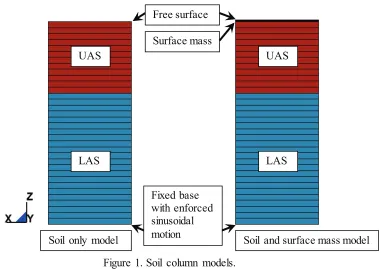
SOIL COLUMN MODELS
The soil column models (as shown in Figure 1) consider an upper alluvial soil (UAS) and a lower alluvial soil (LAS). Both meshes in Figure 1 have 30 feet of UAS and 55 feet of LAS with an element height of
2.5 feet for all of the elements. The surface mass (which is a mass per area) is 0.139 kip•sec2/ft3. This
mass per area is equivalent to evenly distributing a 234,000 ton structure over a footprint of 105,000 ft2.
Figure 1. Soil column models.
An x-direction sinusoidal motion is applied to the fixed base of each model. Multiple model runs are preformed to accommodate input sinusoidal motions at frequencies of 1 Hz, 5 Hz, and 25 Hz. The maximum amplitude differs for each model run to produce a peak shear strain that is near 80% of the
Fixed base with enforced sinusoidal motion
Free surface
Surface mass UAS
LAS
UAS
LAS
maximum value defined in the material properties. This is done to include most of the stress versus strain
data. The motion is defined with a sine wave having an amplitude that linearly varies from zero
amplitude at zero time to its maximum amplitude at one second. The sine wave amplitude is then held constant for two additional seconds. The intent with this time history is to provide a smooth ramp and then time to allow transients to be damped away thereby allowing a steady-state comparison of results
near the end of the time history. (When the SHAKE equations model was developed, the basic
assumption was that of steady-state motion. Therefore, no transient consideration was needed.)
MATERIAL PROPERTIES
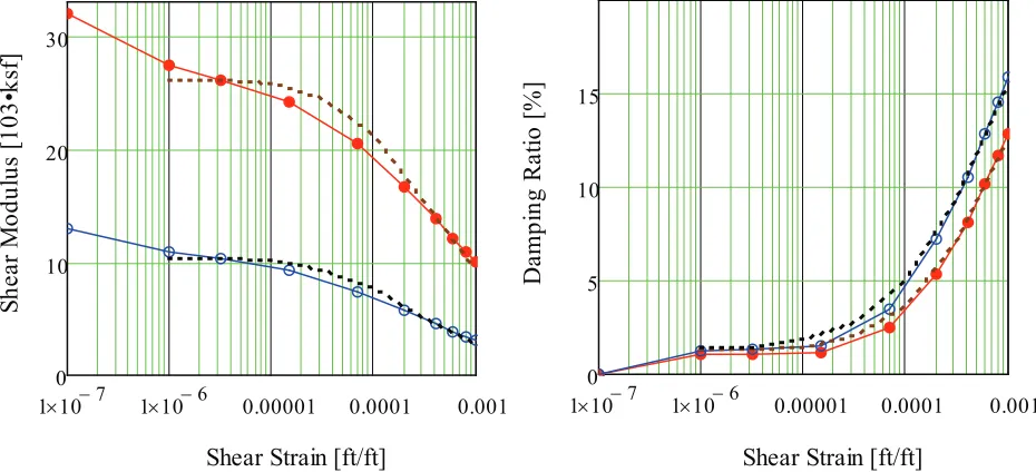
The UAS and LAS material properties for this evaluation are shown in Figures 2 to 4. The linear and nonlinear material properties are defined to be equivalent using Spears et al. (2015). Additionally, the UAS has a density of 118 lbm/ft3, a Poisson’s ratio of 0.25, and an initial bulk modulus of 15,500 ksf.
Likewise, the LAS has a density of 118 lbm/ft3, a Poisson’s ratio of 0.29, and an initial bulk modulus of
32,800 ksf. The bulk modulus values are based on the shear modulus values (shown in Figure 2) for a strain of 10-6 ft/ft.
For this paper, the linear and nonlinear model material properties (shown in Figures 2 to 4) are defined to approximate curve shapes based on Idaho National Laboratory (INL) soils (Payne 2006). These linear
material properties (shown as dotted curves in Figure 2) are for strain values between 10-6 ft/ft and 10-3
ft/ft. In order to approximate low strain (10-6 ft/ft) damping ratio, the material properties used in this
paper include an added lower strain (10-7 ft/ft) data point. This is necessary because the nonlinear model
energy absorption results from soil plasticity. Consequently, the elastic region (where no energy is
absorbed) is made small to allow for energy absorption at low strain (10-6 ft/ft). Given the scatter in the
actual test data, the defined material properties produce a reasonable representation for the soil.
S
h
e
a
r
M
o
d
u
lu
s
[1
0
3
•k
sf]
1 10" !7 1 10" !6 0.00001 0.0001 0.001
0 10 20 30
D
a
m
p
in
g
Ra
ti
o
[%
]
1 10" !7 1 10" !6 0.00001 0.0001 0.001
0 5 10 15
Shear Strain [ft/ft] Shear Strain [ft/ft]
Figure 2. Shear modulus and damping ratio versus shear strain curves for UAS (blue curves with hollow blue circles) and for LAS (red curves with solid circles). Also shown is the linear material properties
S
h
e
a
r
S
tre
ss
[k
sf]
0 0.0002 0.0004 0.0006 0.0008 0.001
0 5 10
E
n
e
rg
y
A
b
so
rb
e
d
p
e
r
Cy
c
le
[ft
•k
ip
/ft
3
]
0 0.0002 0.0004 0.0006 0.0008 0.001
0 0.002 0.004 0.006 0.008
Shear Strain [ft/ft] Shear Strain [ft/ft]
Figure 3. Shear stress and energy absorbed per cycle versus shear strain for UAS (blue curves with hollow blue circles) and LAS (red curves with solid circles).
S
h
e
a
r
S
tre
ss
[k
sf]
0.001
! 0 0.001
10 !
0 10
S
h
e
a
r
S
tre
ss
[k
sf]
0.001
! 0 0.001
10 !
0 10
Shear Strain [ft/ft] Shear Strain [ft/ft]
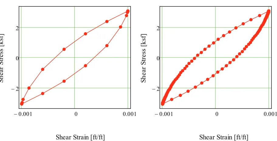
Figure 4. Hysteresis loops for the linear material properties (left-hand plot) and for the nonlinear material properties (right-hand plot). The smaller amplitude (blue curves) are for UAS and the larger amplitude
(red curves) are for LAS.
NONLINEAR LS-DYNA MODELS
allowed in this study.) Likewise, the LAS has a reference pressure and initial mean effective stress in each element of 6.785 ksf and the same flag set relative to the material property stress versus strain curve. The pressure values for the UAS and LAS are selected to minimize the needed vertical motion in the soil nodes to reach static equilibrium under gravitational loading.
Values for other material properties in the material model must also be defined. Given that the stress versus strain curve is held constant, the other material properties become mostly insignificant. For both the UAS and LAS, the off pressure is set at zero. (Note: For mean effective stresses below the cut-off pressure, the shear stresses would be set to zero if the stress versus strain curve is allowed to vary with
mean effective stress.) For both the UAS and LAS, the yield function constants are set at a0= 0, a1= 0,
and a2 = 1. These yield function values are selected simply to put the yield functions in a classical Drucker-Prager form with a zero cut-off pressure. For both the UAS and LAS, the dilation parameters and exponent for bulk modulus pressure sensitivity are set to zero (making them inactive).
Along with the boundary conditions, additional constraints are added to these models. The constraints cause each set of nodes at a given elevation to move horizontally (and vertically) together. This allows the shear (and compressive) plane waves to pass up through the model unimpeded while providing the support that would be received from neighbouring elements in a soil continuum. In this paper, only the vertically propagating shear waves are considered.
The basic idea used by the nonlinear LS-DYNA hysteretic soil constitutive model is based on each element having up to 10 “layers.” Each layer has a unique stiffness, a unique yield stress, and has an elastic/perfectly plastic behaviour based on a kinematic hardening rule. The response of the layers is summed together to produce the post yielding shear stress versus shear strain curve that has been defined for the element. Having the constitutive model defined in this manner produces the realistically shaped hysteresis loops shown in Figure 4.
NONLINEAR RUNGE-KUTTA METHOD MODELS
The nonlinear Runge-Kutta method versions of the soil column models are based on a 10 “layer” LS-DYNA soil constitutive model. Each model is set up as an explicit model using fourth-order Runge-Kutta methods as a solver. The model consists of point masses and nonlinear springs where the point masses occur at the nodal elevations in Figure 1. Each point mass is defined as half the mass in the element above the nodal elevation (if it exists) added to half the mass in the element below the nodal elevation (if it exists). Where applicable, the surface mass is also added to the point mass. The nonlinear springs are defined with the stress versus strain behaviour like the 10 “layer” LS-DYNA soil constitutive model except any number of “layers” may be defined. The time step for the model runs is set at 0.0001 sec and nothing else is done to help ensure model stability.
0.001
! 0 0.001
2 !
0 2
0.001
! 0 0.001
2 !
0 2
S
h
e
a
r
S
tre
ss
[k
sf]
S
h
e
a
r
S
tre
ss
[k
sf]
Shear Strain [ft/ft] Shear Strain [ft/ft]
Figure 5. Hysteresis loops for the 10 layer and 100 layer soil constitutive models respectively.
LINEAR MODELS
The linear versions of the soil column models based on SHAKE equations is evaluated in Mathcad. Using SHAKE equations for displacement and shear stress, a system of linear equations is formed by equating displacement and shear stress at each location where two elements share a common horizontal plane (as shown in Figure 1). Additionally, the bottom displacement is equated to the (constant amplitude) sinusoidal motion and the top shear stress is set to zero (for the model without surface mass) or to the inertial surface mass loads (for the model with surface mass).
In SHAKE, the displacement (and shear stress) is dependent on an upward traveling wave and a downward traveling wave and each has a complex constant assigned to it. These constants are derived using the system of linear equations. When solving the system of linear equations, the results are dependent on the shear modulus and damping ratio in each element. The shear modulus and damping ratio in each element are dependent on the cyclic strain amplitude in the given element. Consequently, an iterative solver is developed to establish the shear modulus and damping ratio in each element that is correct for the cyclic strain amplitude that occurs in the element. For the iterative solver, an initial guess is made for the cyclic strain amplitude in each element. From these strain values and the material properties (shown in Figure 2), the corresponding shear modulus and damping ratio in each element can be found. Next, complex constants are derived with the new shear modulus and damping ratio values. Having the complex constants, the displacement and likewise the cyclic strain amplitude can be found for each element. This concludes the first iteration and the next iteration starts with the new cyclic strain amplitude for each element. After each iteration, the change in cyclic strain amplitude in each element from the previous cycle to the current cycle is found. The amplitudes of these changes are then summed for all of the elements. If this summed value is above 10-12, then another iteration is performed. If this value is below 10-12, then the expectation is that a solution has been found.
The linear LS-DYNA versions of the soil column models use the meshes and boundary conditions shown in Figure 1. Additionally, dashpots go between each pair of vertically consecutive nodes in the meshes (adding four dashpots for each element in a given mesh). The material properties for each linear elastic element and its corresponding dashpots are defined with the shear modulus and damping ratio (derived with the Matchcad model based on SHAKE equations). (Note: Each shear modulus for a given element must be converted to an elastic modulus and each damping ratio for a given element must be converted to a viscous dashpot.)
Given the similarity in results for the SHAKE equations models and linear LS-DYNA models, only the LS-DYNA model results are presented to represent both approaches.
RESULTS AND DISCUSSION
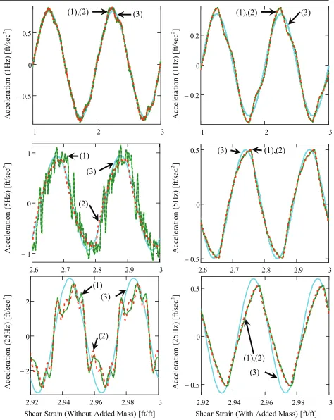
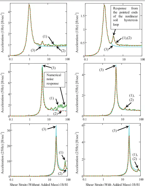
Figures 6 and 7 show the model run results. Figure 6 shows the last two top-of-soil acceleration cycles for the models. Figure 7 shows the top-of-soil 5 % damped response spectra for the models.
For this paper, three different dynamic analyses techniques are reported that represent the five different dynamic analyses techniques that are discussed. These include the nonlinear LS-DYNA results, the nonlinear Runge-Kutta method results with 100 “layers,” and the linear LS-DYNA results (that are representative of the SHAKE based and linear LS-DYNA results). The linear, SHAKE based results represent results that meet the currently accepted ASCE 4 approach used in seismic analysis. The nonlinear LS-DYNA and Runge-Kutta method results represent results that could be used in future seismic analyses following an ASCE 4 approach. The Mathcad 100 layer results are given to provide data on how the results change with a “smoother” hysteresis loop.
Considering Figures 6 and 7, there are significant response differences in the nonlinear 10 “layer” LS-DYNA results, the nonlinear 100 “layer” Runge-Kutta method. One example where a significant difference occurs can be seen in the 5 Hz model (without added mass) response spectra at frequencies greater than 20 Hz. Considering the differences in the acceleration time histories, it is easily seen that there is additional noise in the LS-DYNA results. This noise is considered numerical error caused by the stress versus strain curve not providing “smooth” sides for the hysteresis loop.
Additionally, there are significant response differences where the nonlinear models agree but they significantly differ from the linear model. One example where significant divergence occurs is in the second peak (at a frequency of about 3 Hz) shown in the Figure 7 response spectra for the 1 Hz model (with added mass). This is considered to be a realistic nonlinear response caused by the abrupt tangent stiffness changes at the transition from loading to unloading (represented by the “pointed ends” of the nonlinear soil hysteresis loop). It is clear that the SHAKE type equivalent linear hysteresis model is not capable of capturing this high frequency response (at any strain level) considering its smooth stiffness change at the transition from loading to unloading and considering the results shown in Figures 6 and 7. (The dominant added high frequency response from the pointed ends of the nonlinear soil hysteresis loop causes response peaks at three times the input frequency, five times the input frequency, seven times the input frequency ….)
2.92 2.94 2.96 2.98 3 2
! 0 2
2.92 2.94 2.96 2.98 3
0.5 !
0 0.5
2.6 2.7 2.8 2.9 3
0.5 !
0 0.5
2.6 2.7 2.8 2.9 3
1 !
0 1
1 2 3
0.2 !
0 0.2
1 2 3
0.5 ! 0 0.5 A c c e le ra ti o n (1 H z ) [ft /s e c 2 ] A c c e le ra ti o n (1 H z ) [ft /s e c 2 ] A c c e le ra ti o n (5 H z ) [ft /s e c 2 ] A c c e le ra ti o n (5 H z ) [ft /s e c 2 ] A c c e le ra ti o n (2 5 H z ) [ft /s e c 2 ] A c c e le ra ti o n (2 5 H z ) [ft /s e c 2 ]
Shear Strain (Without Added Mass) [ft/ft] Shear Strain (With Added Mass) [ft/ft]
Figure 6. Top-of-soil acceleration for LS-DYNA nonlinear (1) results (two tone green curve), Mathcad 100 layer (2) results (red dashed-dotted curve), and LS-DYNA linear (3) results (cyan solid curve).
(1),(2)
(3)
(1),(2)
(3)
A c c e le ra ti o n (1 H z ) [ft /s e c 2 ]
0.1 1 10 100
0 1 2 3 4 A c c e le ra ti o n (1 H z ) [ft /s e c 2 ]
0.1 1 10 100
0 0.5 1 1.5 A c c e le ra ti o n (5 H z ) [ft /s e c 2 ]
0.1 1 10 100
0 2 4 6 8 A c c e le ra ti o n (5 H z ) [ft /s e c 2 ]
0.1 1 10 100
0 2 4 A c c e le ra ti o n (2 5 H z ) [ft /s e c 2 ]
0.1 1 10 100
0 10 20 30 A c c e le ra ti o n (2 5 H z ) [ft /s e c 2 ]
0.1 1 10 100
0 2 4 6
Shear Strain (Without Added Mass) [ft/ft] Shear Strain (With Added Mass) [ft/ft]
Figure 7. Top-of-soil, 5 % damped acceleration response spectra for LS-DYNA nonlinear (1) results (two tone green curve), Mathcad 100 layer (2) results (red dashed-dotted curve), and LS-DYNA linear (3)
results (cyan solid curve).
(1)
(3)
(1),(2)
(3)
(1),
(2)
(3)
(1),
(2)
(3)
(1)
(3)
(2)
(1)
(3)
(2)
(2)
Numerical noise responseResponse from
the pointed ends of the nonlinear
soil hysteresis
(Note: The top-of-soil acceleration versus time plots for the Mathcad 100 layer, 25 Hz model without added mass appear as though they still have noise that could be removed with more layers. However, Mathcad 1000 layer results were produced in scoping model runs and they closely matched the Mathcad 100 layer results.)
CONCLUSION
This paper compares linear and nonlinear soil column results. The results show that the nonlinear analysis produces additional high frequency response not seen in linear analysis. Consequently, if the nonlinear soil models produce accurate response relative to actual soil behaviour, high frequency content can be expected even in seismic events that have insignificant high frequency input.
Additionally, to achieve relatively noise free results in nonlinear analysis, the number of soil constitutive model “layers” required is related to the presence of significant structural mass. With significant structural mass on the soil, the LS-DYNA 10 “layer” soil constitutive model produces accurate results. Without significant structural mass on the soil, many more soil constitutive model “layers” may be necessary to produce accurate (noise free) results.
REFERENCES
American Society of Civil Engineers (ASCE) (1998). Seismic Analysis of Safety-Related Nuclear
Structures and Commentary, ASCE/SEI4- 98, Reston, VA, USA.
Deng, N. and Ostadan, F (2000). “SHAKE2000,”Theoretical and User Manual, A Computer Program
for Conducting Equivalent Linear Seismic Response Analyses of Horizontally Layered Soil Deposits. Geotechnical and Hydraulic Engineering Services, Bechtel National Inc., San Francisco, CA, USA.
LSTC (2013). “LS-DYNA, Version smp s R7.00,” LS-DYNA Keyword User’s Manual, Volume II,
Livermore Software Technology Corporation, Livermore, CA, USA.
Mathcad (2011). “Mathcad, Version 15.0 M010,” Parametric Technology Corporation, Needham, MA, USA.
Payne, S. J. (2006). Data and Calculations for Development of Soil Design Basis Earthquake Parameters at RTC. Research Report, INEEL/EXT-03-00943, Revision 2, INL, Idaho Falls, ID, USA.